
Excel для Microsoft 365 Excel для Microsoft 365 для Mac Excel для Интернета Excel 2021 Excel 2021 для Mac Excel 2019 Excel 2019 для Mac Excel 2016 Excel 2016 для Mac Excel 2013 Excel 2010 Excel 2007 Еще…Меньше
Хотя в Excel предлагается большое число встроенных функций, в нем может не быть той функции, которая нужна для ваших вычислений. К сожалению, разработчики Excel не могли предугадать все потребности пользователей. Однако в Excel можно создавать собственные функции, и ниже вы найдете все нужные для этого инструкции.
Пользовательские функции (как и макросы) записываются на языке программирования Visual Basic для приложений (VBA). Они отличаются от макросов двумя вещами. Во-первых, в них используются процедуры Function, а не Sub. Это значит, что они начинаются с оператора Function, а не Sub, и заканчиваются оператором End Function, а не End Sub. Во-вторых, они выполняют различные вычисления, а не действия. Некоторые операторы (например, предназначенные для выбора и форматирования диапазонов) исключаются из пользовательских функций. Из этой статьи вы узнаете, как создавать и применять пользовательские функции. Для создания функций и макросов используется редактор Visual Basic (VBE), который открывается в отдельном окне.
Предположим, что ваша компания предоставляет скидку в размере 10 % клиентам, заказавшим более 100 единиц товара. Ниже мы объясним, как создать функцию для расчета такой скидки.
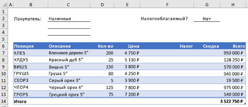
В примере ниже показана форма заказа, в которой перечислены товары, их количество и цена, скидка (если она предоставляется) и итоговая стоимость.
Чтобы создать пользовательскую функцию DISCOUNT в этой книге, сделайте следующее:
-
Нажмите клавиши ALT+F11 (или FN+ALT+F11 на Mac), чтобы открыть редактор Visual Basic, а затем щелкните Insert (Вставка) > Module (Модуль). В правой части редактора Visual Basic появится окно нового модуля.
-
Скопируйте указанный ниже код и вставьте его в новый модуль.
Function DISCOUNT(quantity, price)
   If quantity >=100 Then
     DISCOUNT = quantity * price * 0.1
   Else
     DISCOUNT = 0
   End If

 DISCOUNT = Application.Round(Discount, 2)
End Function
Примечание: Чтобы код было более удобно читать, можно добавлять отступы строк с помощью клавиши TAB. Отступы необязательны и не влияют на выполнение кода. Если добавить отступ, редактор Visual Basic автоматически вставит его и для следующей строки. Чтобы сдвинуть строку на один знак табуляции влево, нажмите SHIFT+TAB.
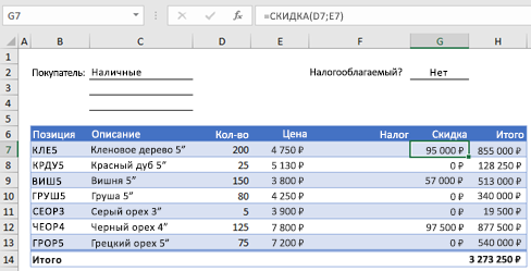
Теперь вы готовы использовать новую функцию DISCOUNT. Закройте редактор Visual Basic, выделите ячейку G7 и введите следующий код:
=DISCOUNT(D7;E7)
Excel вычислит 10%-ю скидку для 200 единиц по цене 47,50 ₽ и вернет 950,00 ₽.
В первой строке кода VBA функция DISCOUNT(quantity, price) указывает, что функции DISCOUNT требуется два аргумента: quantity (количество) и price (цена). При вызове функции в ячейке листа необходимо указать эти два аргумента. В формуле =DISCOUNT(D7;E7) аргумент quantity имеет значение D7, а аргумент price — значение E7. Если скопировать формулу в ячейки G8:G13, вы получите указанные ниже результаты.
Рассмотрим, как Excel обрабатывает эту функцию. При нажатии клавиши ВВОД Excel ищет имя DISCOUNT в текущей книге и определяет, что это пользовательская функция в модуле VBA. Имена аргументов, заключенные в скобки (quantity и price), представляют собой заполнители для значений, на основе которых вычисляется скидка.
Оператор If в следующем блоке кода проверяет аргумент quantity и сравнивает количество проданных товаров со значением 100:
If quantity >= 100 Then
 DISCOUNT = quantity * price * 0.1
Else
 DISCOUNT = 0
End If
Если количество проданных товаров не меньше 100, VBA выполняет следующую инструкцию, которая перемножает значения quantity и price, а затем умножает результат на 0,1:
Discount = quantity * price * 0.1
Результат хранится в виде переменной Discount. Оператор VBA, который хранит значение в переменной, называется оператором назначения, так как он вычисляет выражение справа от знака равенства и назначает результат имени переменной слева от него. Так как переменная Discount называется так же, как и процедура функции, значение, хранящееся в переменной, возвращается в формулу листа, из которой была вызвана функция DISCOUNT.
Если значение quantity меньше 100, VBA выполняет следующий оператор:
Discount = 0
Наконец, следующий оператор округляет значение, назначенное переменной Discount, до двух дробных разрядов:
Discount = Application.Round(Discount, 2)
В VBA нет функции округления, но она есть в Excel. Чтобы использовать округление в этом операторе, необходимо указать VBA, что метод (функцию) Round следует искать в объекте Application (Excel). Для этого добавьте слово Application перед словом Round. Используйте этот синтаксис каждый раз, когда нужно получить доступ к функции Excel из модуля VBA.
Пользовательские функции должны начинаться с оператора Function и заканчиваться оператором End Function. Помимо названия функции, оператор Function обычно включает один или несколько аргументов. Однако вы можете создать функцию без аргументов. В Excel доступно несколько встроенных функций (например, СЛЧИС и ТДАТА), в которых нет аргументов.
После оператора Function указывается один или несколько операторов VBA, которые проверят соответствия условиям и выполняют вычисления с использованием аргументов, переданных функции. Наконец, в процедуру функции следует включить оператор, назначающий значение переменной с тем же именем, что у функции. Это значение возвращается в формулу, которая вызывает функцию.
Количество ключевых слов VBA, которые можно использовать в пользовательских функциях, меньше числа, используемого в макросах. Настраиваемые функции не могут выполнять другие задачи, кроме возврата значения в формулу на этом или в выражение, используемом в другом макросе или функции VBA. Например, пользовательские функции не могут изменять размер окна, редактировать формулу в ячейке, а также изменять шрифт, цвет или узор текста в ячейке. Если в процедуру функции включить такой код действия, функция возвращает #VALUE! ошибку «#ВЫЧИС!».
Единственное действие, которое может выполнять процедура функции (кроме вычислений), — это отображение диалогового окна. Чтобы получить значение от пользователя, выполняющего функцию, можно использовать в ней оператор InputBox. Кроме того, с помощью оператора MsgBox можно выводить сведения для пользователей. Вы также можете использовать настраиваемые диалоговые окна (UserForms), но эта тема выходит за рамки данной статьи.
Даже простые макросы и пользовательские функции может быть сложно понять. Чтобы сделать эту задачу проще, добавьте комментарии с пояснениями. Для этого нужно ввести перед текстом апостроф. Например, ниже показана функция DISCOUNT с комментариями. Благодаря подобным комментариями и вам, и другим будет впоследствии проще работать с кодом VBA. Так, код будет легче понять, если потребуется внести в него изменения.
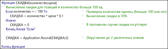
Апостроф указывает приложению Excel на то, что следует игнорировать всю строку справа от него, поэтому вы можете добавлять комментарии в отдельных строках или в правой части строк, содержащих код VBA. Советуем начинать длинный блок кода с комментария, в котором объясняется его назначение, а затем использовать встроенные комментарии для документирования отдельных операторов.
Кроме того, рекомендуется присваивать макросам и пользовательским функциям описательные имена. Например, присвойте макросу название MonthLabels вместо Labels, чтобы более точно указать его назначение. Описательные имена макросов и пользовательских функций особенно полезны, если существует множество процедур с похожим назначением.
То, как документировать макрос и пользовательские функции, имеет личный выбор. Важно принятия определенного способа документации и его согласованного использования.
Для использования настраиваемой функции должна быть открыта книга, содержащая модуль, в котором она была создана. Если книга не открыта, вы получите #NAME? при попытке использования функции. Если вы ссылались на функцию в другой книге, ее имя должно предшествовать названию книги, в которой она находится. Например, при создании функции DISCOUNT в книге Personal.xlsb и вызове ее из другой книги необходимо ввести =personal.xlsb!discount(),а не просто =discount().
Чтобы вставить пользовательскую функцию быстрее (и избежать ошибок), ее можно выбрать в диалоговом окне «Вставка функции». Пользовательские функции доступны в категории «Определенные пользователем»:
Чтобы пользовательские функции всегда были доступны, можно хранить их в отдельной книге, а затем сохранять в качестве надстройки. Затем надстройку можно сделать доступной при запуске Excel. Вот как это сделать:
-
Создав нужные функции, выберите Файл > Сохранить как.
В Excel 2007 нажмите кнопку Microsoft Office, а затем щелкните Сохранить как.
-
В диалоговом окне Сохранить как откройте раскрывающийся список Тип файла и выберите значение Надстройка Excel. Сохраните книгу с запоминающимся именем, таким как MyFunctions, в папке AddIns. Она будет автоматически предложена в диалоговом окне Сохранить как, поэтому вам потребуется только принять расположение, используемое по умолчанию.
-
Сохранив книгу, выберите Файл > Параметры Excel.
В Excel 2007 нажмите кнопку Microsoft Office и щелкните Параметры Excel.
-
В диалоговом окне Параметры Excel выберите категорию Надстройки.
-
В раскрывающемся списке Управление выберите Надстройки Excel. Затем нажмите кнопку Перейти.
-
В диалоговом окне Надстройки установите флажок рядом с именем книги, как показано ниже.


-
Создав нужные функции, выберите Файл > Сохранить как.
-
В диалоговом окне Сохранить как откройте раскрывающийся список Тип файла и выберите значение Надстройка Excel. Сохраните книгу с запоминающимся именем, таким как MyFunctions.
-
Сохранив книгу, выберите Сервис > Надстройки Excel.
-
В диалоговом окне Надстройки нажмите кнопку «Обзор», найдите свою надстройку, нажмите кнопку Открыть, а затем установите флажок рядом с надстройкой в поле Доступные надстройки.
После этого пользовательские функции будут доступны при каждом запуске Excel. Если вы хотите добавить его в библиотеку функций, вернимся в Visual Basic редактора. Если вы заглянуть в Visual Basic редактора Project проводника под заголовком VBAProject, вы увидите модуль с именем файла надстройки. У надстройки будет расширение XLAM.
Дважды щелкните модуль в Project Explorer, чтобы вывести код функций. Чтобы добавить новую функцию, установите точку вставки после оператора End Function, который завершает последнюю функцию в окне кода, и начните ввод. Вы можете создать любое количество функций, и они будут всегда доступны в категории «Определенные пользователем» диалогового окна Вставка функции.
Эта статья основана на главе книги Microsoft Office Excel 2007 Inside Out, написанной Марком Доджем (Mark Dodge) и Крейгом Стинсоном (Craig Stinson). В нее были добавлены сведения, относящиеся к более поздним версиям Excel.
Дополнительные сведения
Вы всегда можете задать вопрос специалисту Excel Tech Community или попросить помощи в сообществе Answers community.
Нужна дополнительная помощь?
Введение
Всем нам приходится — кому реже, кому чаще — повторять одни и те же действия и операции в Excel. Любая офисная работа предполагает некую «рутинную составляющую» — одни и те же еженедельные отчеты, одни и те же действия по обработке поступивших данных, заполнение однообразных таблиц или бланков и т.д. Использование макросов и пользовательских функций позволяет автоматизировать эти операции, перекладывая монотонную однообразную работу на плечи Excel. Другим поводом для использования макросов в вашей работе может стать необходимость добавить в Microsoft Excel недостающие, но нужные вам функции. Например функцию сборки данных с разных листов на один итоговый лист, разнесения данных обратно, вывод суммы прописью и т.д.
Макрос — это запрограммированная последовательность действий (программа, процедура), записанная на языке программирования Visual Basic for Applications (VBA). Мы можем запускать макрос сколько угодно раз, заставляя Excel выполнять последовательность любых нужных нам действий, которые нам не хочется выполнять вручную.
В принципе, существует великое множество языков программирования (Pascal, Fortran, C++, C#, Java, ASP, PHP…), но для всех программ пакета Microsoft Office стандартом является именно встроенный язык VBA. Команды этого языка понимает любое офисное приложение, будь то Excel, Word, Outlook или Access.
Способ 1. Создание макросов в редакторе Visual Basic
Для ввода команд и формирования программы, т.е. создания макроса необходимо открыть специальное окно — редактор программ на VBA, встроенный в Microsoft Excel.
- В старых версиях (Excel 2003 и старше) для этого идем в меню Сервис — Макрос — Редактор Visual Basic (Toos — Macro — Visual Basic Editor).
- В новых версиях (Excel 2007 и новее) для этого нужно сначала отобразить вкладку Разработчик (Developer). Выбираем Файл — Параметры — Настройка ленты (File — Options — Customize Ribbon) и включаем в правой части окна флажок Разработчик (Developer). Теперь на появившейся вкладке нам будут доступны основные инструменты для работы с макросами, в том числе и нужная нам кнопка Редактор Visual Basic (Visual Basic Editor)
 :
:
 :
:К сожалению, интерфейс редактора VBA и файлы справки не переводятся компанией Microsoft на русский язык, поэтому с английскими командами в меню и окнах придется смириться:

Макросы (т.е. наборы команд на языке VBA) хранятся в программных модулях. В любой книге Excel мы можем создать любое количество программных модулей и разместить там наши макросы. Один модуль может содержать любое количество макросов. Доступ ко всем модулям осуществляется с помощью окна Project Explorer в левом верхнем углу редактора (если его не видно, нажмите CTRL+R). Программные модули бывают нескольких типов для разных ситуаций:
- Обычные модули — используются в большинстве случаев, когда речь идет о макросах. Для создания такого модуля выберите в меню Insert — Module. В появившееся окно нового пустого модуля можно вводить команды на VBA, набирая их с клавиатуры или копируя их из другого модуля, с этого сайта или еще откуда нибудь:

- Модуль Эта книга — также виден в левом верхнем углу редактора Visual Basic в окне, которое называется Project Explorer. В этот модуль обычно записываются макросы, которые должны выполнятся при наступлении каких-либо событий в книге (открытие или сохранение книги, печать файла и т.п.):

- Модуль листа — доступен через Project Explorer и через контекстное меню листа, т.е. правой кнопкой мыши по ярлычку листа — команда Исходный текст (View Source). Сюда записывают макросы, которые должны выполняться при наступлении определенных событий на листе (изменение данных в ячейках, пересчет листа, копирование или удаление листа и т.д.)


Обычный макрос, введенный в стандартный модуль выглядит примерно так:

Давайте разберем приведенный выше в качестве примера макрос Zamena:
- Любой макрос должен начинаться с оператора Sub, за которым идет имя макроса и список аргументов (входных значений) в скобках. Если аргументов нет, то скобки надо оставить пустыми.
- Любой макрос должен заканчиваться оператором End Sub.
- Все, что находится между Sub и End Sub — тело макроса, т.е. команды, которые будут выполняться при запуске макроса. В данном случае макрос выделяет ячейку заливает выделенных диапазон (Selection) желтым цветом (код = 6) и затем проходит в цикле по всем ячейкам, заменяя формулы на значения. В конце выводится окно сообщения (MsgBox).
С ходу ясно, что вот так сразу, без предварительной подготовки и опыта в программировании вообще и на VBA в частности, сложновато будет сообразить какие именно команды и как надо вводить, чтобы макрос автоматически выполнял все действия, которые, например, Вы делаете для создания еженедельного отчета для руководства компании. Поэтому мы переходим ко второму способу создания макросов, а именно…
Способ 2. Запись макросов макрорекордером
Макрорекордер — это небольшая программа, встроенная в Excel, которая переводит любое действие пользователя на язык программирования VBA и записывает получившуюся команду в программный модуль. Если мы включим макрорекордер на запись, а затем начнем создавать свой еженедельный отчет, то макрорекордер начнет записывать команды вслед за каждым нашим действием и, в итоге, мы получим макрос создающий отчет как если бы он был написан программистом. Такой способ создания макросов не требует знаний пользователя о программировании и VBA и позволяет пользоваться макросами как неким аналогом видеозаписи: включил запись, выполнил операци, перемотал пленку и запустил выполнение тех же действий еще раз. Естественно у такого способа есть свои плюсы и минусы:
- Макрорекордер записывает только те действия, которые выполняются в пределах окна Microsoft Excel. Как только вы закрываете Excel или переключаетесь в другую программу — запись останавливается.
- Макрорекордер может записать только те действия, для которых есть команды меню или кнопки в Excel. Программист же может написать макрос, который делает то, что Excel никогда не умел (сортировку по цвету, например или что-то подобное).
- Если во время записи макроса макрорекордером вы ошиблись — ошибка будет записана. Однако смело можете давить на кнопку отмены последнего действия (Undo) — во время записи макроса макрорекордером она не просто возрвращает Вас в предыдущее состояние, но и стирает последнюю записанную команду на VBA.
Чтобы включить запись необходимо:
- в Excel 2003 и старше — выбрать в меню Сервис — Макрос — Начать запись (Tools — Macro — Record New Macro)
- в Excel 2007 и новее — нажать кнопку Запись макроса (Record macro) на вкладке Разработчик (Developer)
Затем необходимо настроить параметры записываемого макроса в окне Запись макроса:

- Имя макроса — подойдет любое имя на русском или английском языке. Имя должно начинаться с буквы и не содержать пробелов и знаков препинания.
- Сочетание клавиш — будет потом использоваться для быстрого запуска макроса. Если забудете сочетание или вообще его не введете, то макрос можно будет запустить через меню Сервис — Макрос — Макросы — Выполнить (Tools — Macro — Macros — Run) или с помощью кнопки Макросы (Macros) на вкладке Разработчик (Developer) или нажав ALT+F8.
- Сохранить в… — здесь задается место, куда будет сохранен текст макроса, т.е. набор команд на VBA из которых и состоит макрос.:
- Эта книга — макрос сохраняется в модуль текущей книги и, как следствие, будет выполнятся только пока эта книга открыта в Excel
- Новая книга — макрос сохраняется в шаблон, на основе которого создается любая новая пустая книга в Excel, т.е. макрос будет содержаться во всех новых книгах, создаваемых на данном компьютере начиная с текущего момента
- Личная книга макросов — это специальная книга Excel с именем Personal.xls, которая используется как хранилище макросов. Все макросы из Personal.xls загружаются в память при старте Excel и могут быть запущены в любой момент и в любой книге.
После включения записи и выполнения действий, которые необходимо записать, запись можно остановить командой Остановить запись (Stop Recording).
Запуск и редактирование макросов
Управление всеми доступными макросами производится в окне, которое можно открыть с помощью кнопки Макросы (Macros) на вкладке Разработчик (Developer) или — в старых версиях Excel — через меню Сервис — Макрос — Макросы (Tools — Macro — Macros):

- Любой выделенный в списке макрос можно запустить кнопкой Выполнить (Run).
- Кнопка Параметры (Options) позволяет посмотреть и отредактировать сочетание клавиш для быстрого запуска макроса.
- Кнопка Изменить (Edit) открывает редактор Visual Basic (см. выше) и позволяет просмотреть и отредактировать текст макроса на VBA.
Создание кнопки для запуска макросов
Чтобы не запоминать сочетание клавиш для запуска макроса, лучше создать кнопку и назначить ей нужный макрос. Кнопка может быть нескольких типов:
Кнопка на панели инструментов в Excel 2003 и старше
Откройте меню Сервис — Настройка (Tools — Customize) и перейдите на вкладку Команды (Commands). В категории Макросы легко найти веселый желтый «колобок» — Настраиваемую кнопку (Custom button):

Перетащите ее к себе на панель инструментов и затем щелкните по ней правой кнопкой мыши. В контекстом меню можно назначить кнопке макрос, выбрать другой значок и имя:

Кнопка на панели быстрого доступа в Excel 2007 и новее
Щелкните правой кнопкой мыши по панели быстрого доступа в левом верхнем углу окна Excel и выберите команду Настройка панели быстрого доступа (Customise Quick Access Toolbar):

Затем в открывшемся окне выберите категорию Макросы и при помощи кнопки Добавить (Add) перенесите выбранный макрос в правую половину окна, т.е. на панель быстрого доступа:

Кнопка на листе
Этот способ подходит для любой версии Excel. Мы добавим кнопку запуска макроса прямо на рабочий лист, как графический объект. Для этого:
- В Excel 2003 и старше — откройте панель инструментов Формы через меню Вид — Панели инструментов — Формы (View — Toolbars — Forms)
- В Excel 2007 и новее — откройте выпадающий список Вставить (Insert) на вкладке Разработчик (Developer)
Выберите объект Кнопка (Button):

Затем нарисуйте кнопку на листе, удерживая левую кнопку мыши. Автоматически появится окно, где нужно выбрать макрос, который должен запускаться при щелчке по нарисованной кнопке.
Создание пользовательских функций на VBA
Создание пользовательских функций или, как их иногда еще называют, UDF-функций (User Defined Functions) принципиально не отличается от создания макроса в обычном программном модуле. Разница только в том, что макрос выполняет последовательность действий с объектами книги (ячейками, формулами и значениями, листами, диаграммами и т.д.), а пользовательская функция — только с теми значениями, которые мы передадим ей как аргументы (исходные данные для расчета).
Чтобы создать пользовательскую функцию для расчета, например, налога на добавленную стоимость (НДС) откроем редактор VBA, добавим новый модуль через меню Insert — Module и введем туда текст нашей функции:

Обратите внимание, что в отличие от макросов функции имеют заголовок Function вместо Sub и непустой список аргументов (в нашем случае это Summa). После ввода кода наша функция становится доступна в обычном окне Мастера функций (Вставка — Функция) в категории Определенные пользователем (User Defined):

После выбора функции выделяем ячейки с аргументами (с суммой, для которой надо посчитать НДС) как в случае с обычной функцией:

Skip to content
В решении многих задач обычные функции Excel не всегда могут помочь. Если существующих функций недостаточно, Excel позволяет добавить новые настраиваемые пользовательские функции (UDF). Они делают вашу работу легче.
Мы расскажем, как можно их создать, какие они бывают и как использовать их, чтобы ваша работа стала проще. Узнайте, как записать и использовать пользовательские функции, которые многие называют макросами..
- Что такое пользовательская функция
- Для чего ее используют?
- Как создать пользовательскую функцию в VBA?
- Как использовать пользовательскую функцию в формуле?
- Какие бывают типы пользовательских функций
Что такое пользовательская функция в Excel?
На момент написания этой статьи Excel предлагает вам более 450 различных функций. С их помощью вы можете выполнять множество различных операций. Но разработчики Microsoft Excel не могли предвидеть все задачи, которые нам нужно решать. Думаю, что многие из вас встречались с этими проблемами:
- не все данные могут быть обработаны стандартными функциями (например, даты до 1900 года).
- формулы могут быть весьма длинными и сложными. Их невозможно запомнить, трудно понять и сложно изменить для решения новой задачи.
- Не все задачи могут быть решены при помощи стандартных функций Excel (в частности, нельзя извлечь интернет-адрес из гиперссылки).
- Невозможно автоматизировать часто повторяющиеся стандартные операции (импорт данных из бухгалтерской программы на лист Excel, форматирование дат и чисел, удаление лишних колонок).
Как можно решить эти проблемы?
- Для очень сложных формул многие пользователи создают архив рабочих книг с примерами. Они копируют оттуда нужную формулу и применяют ее в своей таблице.
- Создание макросов VBA.
- Создание пользовательских функций при помощи редактора VBA.
Хотя первые два варианта кажутся вам знакомыми, третий может вызвать некоторую путаницу. Итак, давайте подробнее рассмотрим настраиваемые функции в Excel и решим, стоит ли их использовать.
Пользовательская функция – это настраиваемый код, который принимает исходные данные, производит вычисление и возвращает желаемый результат.
Исходными данными могут быть числа, текст, даты, логические значения, массивы. Результатом вычислений может быть значение любого типа, с которым работает Excel, или массив таких значений.
Другими словами, пользовательская функция – это своего рода модернизация стандартных функций Excel. Вы можете использовать ее, когда возможностей обычных функций недостаточно. Основное ее назначение – дополнить и расширить возможности Excel, выполнить действия, которые невозможны со стандартными возможностями.
Существует несколько способов создания собственных функций:
- при помощи Visual Basic for Applications (VBA). Этот способ описывается в данной статье.
- с использованием замечательной функции LAMBDA, которая появилась в Office365.
- при помощи Office Scripts. На момент написания этой статьи они доступны в Excel Online в подписке на Office365.
Посмотрите на скриншот ниже, чтобы увидеть разницу между двумя способами извлечения чисел — с использованием формулы и пользовательской функции ExtractNumber().

Даже если вы сохранили эту огромную формулу в своем архиве, вам нужно ее найти, скопировать и вставить, а затем аккуратно поправить все ссылки на ячейки. Согласитесь, это потребует затрат времени, да и ошибки не исключены.
А на ввод функции вы потратите всего несколько секунд.
Для чего можно использовать?
Вы можете использовать настраиваемую функцию одним из следующих способов:
- В формуле, где она может брать исходные данные из вашего рабочего листа и возвращать рассчитанное значение или массив значений.
- Как часть кода макроса VBA или другой пользовательской функции.
- В формулах условного форматирования.
- Для хранения констант и списков данных.
Для чего нельзя использовать пользовательские функции:
- Любого изменения другой ячейки, кроме той, в которую она записана,
- Изменения имени рабочего листа,
- Копирования листов рабочей книги,
- Поиска и замены значений,
- Изменения форматирования ячейки, шрифта, фона, границ, включения и отключения линий сетки,
- Вызова и выполнения макроса VBA, если его выполнение нарушит перечисленные выше ограничения. Если вы используете строку кода, который не может быть выполнен, вы можете получить ошибку RUNTIME ERROR либо просто одну из стандартных ошибок (например, #ЗНАЧЕН!).
Как создать пользовательскую функцию в VBA?
Прежде всего, необходимо открыть редактор Visual Basic (сокращенно — VBE). Обратите внимание, что он открывается в новом окне. Окно Excel при этом не закрывается.
Самый простой способ открыть VBE — использовать комбинацию клавиш. Это быстро и всегда доступно. Нет необходимости настраивать ленту или панель инструментов быстрого доступа. Нажмите Alt + F11 на клавиатуре, чтобы открыть VBE. И снова нажмите Alt + F11, когда редактор открыт, чтобы вернуться назад в окно Excel.

После открытия VBE вам нужно добавить новый модуль. В него вы будете записывать ваш код. Щелкните правой кнопкой мыши на панели проекта VBA слева и выберите «Insert», затем появившемся справа окне — “Module”.
Справа появится пустое окно модуля, в котором вы и будете создавать свою функцию.
Прежде чем начать, напомним правила, по которым создается функция.
- Пользовательская функция всегда начинается с оператора Function и заканчивается инструкцией End Function.
- После оператора Function указывают имя функции. Это название, которое вы создаете и присваиваете, чтобы вы могли идентифицировать и использовать ее позже. Оно не должно содержать пробелов. Если вы хотите разделять слова, используйте подчеркивания. Например, Count_Words.
- Кроме того, это имя также не может совпадать с именами стандартных функций Excel. Если вы сделаете это, то всегда будет выполняться стандартная функция.
- Имя пользовательской функции не может совпадать с адресами ячеек на листе. Например, имя ABC1234 невозможно присвоить.
- Настоятельно рекомендуется давать описательные имена. Тогда вы можете легко выбрать нужное из длинного списка функций. Например, имя CountWords позволяет легко понять, что она делает, и при необходимости применить ее для подсчета слов.
- Далее в скобках обычно перечисляют аргументы. Это те данные, с которыми она будет работать. Может быть один или несколько аргументов. Если у вас несколько аргументов, их нужно перечислить через запятую.
- После этого обычно объявляются переменные, которые использует пользовательская функция. Указывается тип этих переменных – число, дата, текст, массив.
- Если операторы, которые вы используете внутри вашей функции, не используют никакие аргументы (например, NOW (СЕЙЧАС), TODAY (СЕГОДНЯ) или RAND (СЛЧИС)), то вы можете создать функцию без аргументов. Также аргументы не нужны, если вы используете функцию для хранения констант (например, числа Пи).
- Затем записывают несколько операторов VBA, которые выполняют вычисления с использованием переданных аргументов.
- В конце вы должны вставить оператор, который присваивает итоговое значение переменной с тем же именем, что и имя функции. Это значение возвращается в формулу, из которой была вызвана пользовательская функция.
- Записанный вами код может включать комментарии. Они помогут вам не забыть назначение функции и отдельных ее операторов. Если вы в будущем захотите внести какие-то изменения, комментарии будут вам очень полезны. Комментарий всегда начинается с апострофа (‘). Апостроф указывает Excel игнорировать всё, что записано после него, и до конца строки.
Теперь давайте попробуем создать вашу первую собственную формулу. Для начала мы создаем код, который будет подсчитывать количество слов в диапазоне ячеек.
Для этого в окно модуля вставим этот код:
Function CountWords(NumRange As Range) As Long
Dim rCell As Range, lCount As Long
    For Each rCell In NumRange
        lCount = lCount + _
          Len(WorksheetFunction.Trim(rCell)) - Len(Replace(WorksheetFunction.Trim(rCell), " ", "")) + 1
    Next rCell
CountWords = lCount
End Function
Я думаю, здесь могут потребоваться некоторые пояснения.
Код функции всегда начинается с пользовательской процедуры Function. В процедуре Function мы делаем описание новой функции.
В начале мы должны записать ее имя: CountWords.
Затем в скобках указываем, какие исходные данные она будет использовать. NumRange As Range означает, что аргументом будет диапазон значений. Сюда нужно передать только один аргумент — диапазон ячеек, в котором будет происходить подсчёт.
As Long указывает, что результат выполнения функции CountWords будет целым числом.
Во второй строке кода мы объявляем переменные.
Оператор Dim объявляет переменные:
rCell — переменная диапазона ячеек, в котором мы будем подсчитывать слова.
lCount — переменная целое число, в которой будет записано число слов.
Цикл For Each… Next предназначен для выполнения вычислений по отношению к каждому элементу из группы элементов (нашего диапазона ячеек). Этот оператор цикла применяется, когда неизвестно количество элементов в группе. Начинаем с первого элемента, затем берем следующий и так повторяем до самого последнего значения. Цикл повторяется столько раз, сколько ячеек имеется во входном диапазоне.
Внутри этого цикла с значением каждой ячейки выполняется операция, которая вычисляет количество слов:
Len(WorksheetFunction.Trim(rCell)) — Len(Replace(WorksheetFunction.Trim(rCell), » «, «»)) + 1
Как видите, это обычная формула Excel, которая использует стандартные средства работы с текстом: LEN, TRIM и REPLACE. Это английские названия знакомых нам русскоязычных ДЛСТР, СЖПРОБЕЛЫ и ЗАМЕНИТЬ. Вместо адреса ячейки рабочего листа используем переменную диапазона rCell. То есть, для каждой ячейки диапазона мы последовательно считаем количество слов в ней.
Подсчитанные числа суммируются и сохраняются в переменной lCount:
lCount = lCount + Len(WorksheetFunction.Trim(rCell)) — Len(Replace(WorksheetFunction.Trim(rCell), » «, «»)) + 1
Когда цикл будет завершен, значение переменной присваивается функции.
CountWords = lCount
Функция возвращает в ячейку рабочего листа значение этой переменной, то есть общее количество слов.
Именно эта строка кода гарантирует, что функция вернет значение lCount обратно в ячейку, из которой она была вызвана.
Закрываем наш код с помощью «End Function».
Как видите, не очень сложно.
Сохраните вашу работу. Для этого просто нажмите кнопку “Save” на ленте VB редактора.
После этого вы можете закрыть окно редактора. Для этого можно использовать комбинацию клавиш Alt+Q. Или просто вернитесь на лист Excel, нажав Alt+F11.
Вы можете сравнить работу с пользовательской функцией CountWords и подсчет количества слов в диапазоне при помощи формул.
Как использовать пользовательскую функцию в формуле?
Когда вы создали пользовательскую, она становится доступной так же, как и другие стандартные функции Excel. Сейчас мы узнаем, как создавать с ее помощью собственные формулы.
Чтобы использовать ее, у вас есть две возможности.
Первый способ. Нажмите кнопку fx в строке формул. Среди появившихся категорий вы увидите новую группу — Определённые пользователем. И внутри этой категории вы можете увидеть нашу новую пользовательскую функцию CountWords.

Второй способ. Вы можете просто записать эту функцию в ячейку так же, как вы это делаете обычно. Когда вы начинаете вводить имя, Excel покажет вам имя пользовательской в списке соответствующих функций. В приведенном ниже примере, когда я ввел = cou , Excel показал мне список подходящих функций, среди которых вы видите и CountWords.

Можно посчитать этой же функцией и количество слов в диапазоне. Запишите в ячейку С3:
=CountWords(A2:A5)
Нажмите Enter.
Мы только что указали функцию и установили диапазон, и вот результат подсчета: 14 слов.
Для сравнения в C1 я записал формулу массива, при помощи которой мы также можем подсчитать количество слов в диапазоне.

Как видите, результаты одинаковы. Только использовать CountWords() гораздо проще и быстрее.
Различные типы пользовательских функций с использованием VBA.
Теперь мы познакомимся с разными типами пользовательских функций в зависимости от используемых ими аргументов и результатов, которые они возвращают.
Без аргументов.
В Excel есть несколько стандартных функций, которые не требуют аргументов (например, СЛЧИС , СЕГОДНЯ , СЕЧАС). Например, СЛЧИС возвращает случайное число от 0 до 1. СЕГОДНЯ вернет текущую дату. Вам не нужно передавать им какие-либо значения.
Вы можете создать такую функцию и в VBA.
Ниже приведен код, который запишет в ячейку имя вашего рабочего листа.
Function SheetName() as String
    Application.Volatile
    SheetName = Application.Caller.Worksheet.Name
End Function
Или же можно использовать такой код:
SheetName = ActiveSheet.NameОбратите внимание, что в скобках после имени нет ни одного аргумента. Здесь не требуется никаких аргументов, так как результат, который нужно вернуть, не зависит от каких-либо значений в вашем рабочем файле.
Приведенный выше код определяет результат функции как тип данных String (поскольку желаемый результат — это имя файла, которое является текстом). Если вы не укажете тип данных, то Excel будет определять его самостоятельно.
С одним аргументом.
Создадим простую функцию, которая работает с одним аргументом, то есть с одной ячейкой. Наша задача – извлечь из текстовой строки последнее слово.
Function ReturnLastWord(The_Text As String)
Dim stLastWord As String
'Extracts the LAST word from a text string
    stLastWord = StrReverse(The_Text)
    stLastWord = Left(stLastWord, InStr(1, stLastWord, " ", vbTextCompare))
    ReturnLastWord = StrReverse(Trim(stLastWord))
End Function
Аргумент The_Text — это значение выбранной ячейки. Указываем, что это должно быть текстовое значение (As String).
Оператор StrReverse возвращает текст с обратным порядком следования знаков. Далее InStr определяет позицию первого пробела. При помощи Left получаем все знаки заканчивая первым пробелом. Затем удаляем пробелы при помощи Trim. Вновь меняем порядок следования символов при помощи StrReverse. Получаем последнее слово из текста.
Поскольку эта функция принимает значение ячейки, нам не нужно использовать здесь Application.Volatile. Как только аргумент изменится, функция автоматически обновится.
Использование массива в качестве аргумента.
Многие функции Excel используют массивы значений как аргументы. Вспомните функции СУММ, СУММЕСЛИ, СУММПРОИЗВ.
Мы уже рассмотрели эту ситуацию выше, когда учились создавать пользовательскую функцию для подсчета количества слов в диапазоне ячеек.
Приведённый ниже код создает функцию, которая суммирует все чётные числа в указанном диапазоне ячеек.
Function SumEven(NumRange as Range)
 Dim RngCell As Range
 For Each RngCell In NumRange
 If IsNumeric(RngCell.Value) Then
 If RngCell.Value Mod 2 = 0 Then
 Result = Result + RngCell.Value
 End If
 End If
 Next RngCell
 SumEven = Result
 End Function
Аргумент NumRange указан как Range. Это означает, что функция будет использовать массив исходных данных. Необходимо отметить, что можно использовать также тип переменной Variant. Это выглядит как
Function SumEven(NumRange as Variant)Тип Variant обеспечивает «безразмерный» контейнер для хранения данных. Такая переменная может хранить данные любого из допустимых в VBA типов, включая числовые значения, текст, даты и массивы. Более того, одна и та же такая переменная в одной и той же программе в разные моменты может хранить данные различных типов. Excel самостоятельно будет определять, какие данные передаются в функцию.
В коде есть цикл For Each … Next, который берет каждую ячейку и проверяет, есть ли в ней число. Если это не так, то ничего не происходит, и он переходит к следующей ячейке. Если найдено число, он проверяет, четное оно или нет (с помощью функции MOD).
Все чётные числа суммируются в переменной Result.
Когда цикл будет закончен, значение Result присваивается переменной SumEven и передаётся функции.
С несколькими аргументами.
Большинство функций Excel имеет несколько аргументов. Не являются исключением и пользовательские функции. Поэтому так важно уметь создавать собственные функции с несколькими аргументами.
В приведенном ниже коде создается функция, которая выбирает максимальное число в заданном интервале.
Она имеет 3 аргумента: диапазон значений, нижняя граница числового интервала, верхняя граница интервала.
Function GetMaxBetween(rngCells As Range, MinNum, MaxNum)
Dim NumRange As Range
Dim vMax
Dim arrNums()
Dim i As Integer
ReDim arrNums(rngCells.Count)
    For Each NumRange In rngCells
     vMax = NumRange
        Select Case vMax
           Case MinNum + 0.01 To MaxNum - 0.01
              arrNums(i) = vMax
              i = i + 1
           Case Else
               GetMaxBetween = 0
           End Select
    Next NumRange
    GetMaxBetween = WorksheetFunction.Max(arrNums)
End Function
Здесь мы используем три аргумента. Первый из них — rngCells As Range. Это диапазон ячеек, в которых нужно искать максимальное значение. Второй и третий аргумент (MinNum, MaxNum) указаны без объявления типа. Это означает, что по умолчанию к ним будет применён тип данных Variant. В VBA используется 6 различных числовых типов данных. Указывать только один из них — это значит ограничить применение функции. Поэтому более целесообразно, если Excel сам определит тип числовых данных.
Цикл For Each … Next последовательно просматривает все значения в выбранном диапазоне. Числа, которые находятся в интервале от максимального до минимального значения, записываются в специальный массив arrNums. При помощи стандартного оператора MAX в этом массиве находим наибольшее число.
С обязательными и необязательными аргументами.
Чтобы понять, что такое необязательный аргумент, вспомните функцию ВПР (VLOOKUP). Её четвертый аргумент [range_lookup] является необязательным. Если вы не укажете один из обязательных аргументов, получите ошибку. Но если вы пропустите необязательный аргумент, всё будет работать.
Но необязательные аргументы не бесполезны. Они позволяют вам выбирать вариант расчётов.
Например, в функции ВПР, если вы не укажете четвертый аргумент, будет выполнен приблизительный поиск. Если вы укажете его как ЛОЖЬ (или 0), то будет найдено точное совпадение.
Если в вашей пользовательской функции есть хотя бы один обязательный аргумент, то он должен быть записан в начале. Только после него могут идти необязательные.
Чтобы сделать аргумент необязательным, вам просто нужно добавить «Optional» перед ним.
Теперь давайте посмотрим, как создать функцию в VBA с необязательными аргументами.
Function GetText(textCell As Range, Optional CaseText = False) As String
Dim StringLength As Integer
Dim Result As String
StringLength = Len(textCell)
For i = 1 To StringLength
If Not (IsNumeric(Mid(textCell, i, 1))) Then Result = Result & Mid(textCell, i, 1)
Next i
If CaseText = True Then Result = UCase(Result)
GetText = Result
End Function
Этот код извлекает текст из ячейки. Optional CaseText = False означает, что аргумент CaseText необязательный. По умолчанию его значение установлено FALSE.
Если необязательный аргумент CaseText имеет значение TRUE, то возвращается результат в верхнем регистре. Если необязательный аргумент FALSE или опущен, результат остается как есть, без изменения регистра символов.
Думаю, что у вас возник вопрос: «Могут ли в пользовательской функции быть только необязательные аргументы?». Ответ смотрите ниже.
Только с необязательным аргументом.
Насколько мне известно, нет встроенной функции Excel, которая имеет только необязательные аргументы. Здесь я могу ошибаться, но я не могу припомнить ни одной такой.
Но при создании пользовательской такое возможно.
Перед вами функция, которая записывает в ячейку имя пользователя.
Function UserName(Optional Uppercase As Variant)
    If IsMissing(Uppercase) Then Uppercase = False
    UserName = Application.UserName
    If Uppercase Then UserName = UCase(UserName)
End Function
Как видите, здесь есть только один аргумент Uppercase, и он не обязательный.
Если аргумент равен FALSE или опущен, то имя пользователя возвращается без каких-либо изменений. Если же аргумент TRUE, то имя возвращается в символах верхнего регистра (с помощью VBA-оператора Ucase). Обратите внимание на вторую строку кода. Она содержит VBA-функцию IsMissing, которая определяет наличие аргумента. Если аргумент отсутствует, оператор присваивает переменной Uppercase значение FALSE.
Можно предложить и другой вариант этой функции.
Function UserName(Optional Uppercase As Variant)
    If IsMissing(Uppercase) Then Uppercase = False
    UserName = Application.UserName
    If Uppercase Then UserName = UCase(UserName)
End Function
В этом случае необязательный аргумент имеет значение по умолчанию FALSE. Если функция будет введена без аргументов, то значение FALSE будет использовано по умолчанию и имя пользователя будет получено без изменения регистра символов. Если будет введено любое значение кроме нуля, то все символы будут преобразованы в верхний регистр.
Возвращаемое значение — массив.
В VBA имеется весьма полезная функция — Array. Она возвращает значение с типом данных Variant, которое представляет собой массив (т.е. несколько значений).
Пользовательские функции, которые возвращают массив, весьма полезны при хранении массивов значений. Например, Months() вернёт массив названий месяцев:
Function Months() As Variant
Months = Array("Январь", "Февраль", "Март", "Апрель", "Май", "Июнь", _
"Июль", "Август", "Сентябрь", "Октябрь", "Ноябрь", "Декабрь")
End Function
Обратите внимание, что функция выводит данные в строке, по горизонтали.

В Office365 и выше можно вводить как обычную формулу, в более ранних версиях – как формулу массива.
А если необходим вертикальный массив значений?
Мы уже говорили ранее, что созданные нами функции можно использовать в формулах Excel вместе со стандартными.
Используем Months() как аргумент функции ТРАНСП:
=ТРАНСП(Months())
![]()
Как можно использовать пользовательские функции с массивом данных? Можно применять их для ввода данных в таблицу, как показано на рисунке выше. К примеру, в отчёте о продажах не нужно вручную писать названия месяцев.
Можно получить название месяца по его номеру. Например, в ячейке A1 записан номер месяца. Тогда название месяца можно получить при помощи формулы
=ИНДЕКС(Months();1;A1)
Альтернативный вариант этой формулы:
=ИНДЕКС( {«Январь»; «Февраль»; «Март»; «Апрель»; «Май»; «Июнь»; «Июль»; «Август»; «Сентябрь»; «Октябрь»; «Ноябрь»; «Декабрь»};1;A1)
Согласитесь, написанная нами функция делает формулу Excel значительно проще.
Эта статья откроет серию материалов о пользовательских функциях. Если мне удалось убедить вас, что это стоит использовать или вы хотели бы попробовать что-то новое в Excel, следите за обновлениями;)
 Сумма по цвету и подсчёт по цвету в Excel — В этой статье вы узнаете, как посчитать ячейки по цвету и получить сумму по цвету ячеек в Excel. Эти решения работают как для окрашенных вручную, так и с условным форматированием. Если…
  Проверка данных с помощью регулярных выражений — В этом руководстве показано, как выполнять проверку данных в Excel с помощью регулярных выражений и пользовательской функции RegexMatch. Когда дело доходит до ограничения пользовательского ввода на листах Excel, проверка данных очень полезна. Хотите… Поиск и замена в Excel с помощью регулярных выражений — В этом руководстве показано, как быстро добавить пользовательскую функцию в свои рабочие книги, чтобы вы могли использовать регулярные выражения для замены текстовых строк в Excel. Когда дело доходит до замены… Как извлечь строку из текста при помощи регулярных выражений — В этом руководстве вы узнаете, как использовать регулярные выражения в Excel для поиска и извлечения части текста, соответствующего заданному шаблону. Microsoft Excel предоставляет ряд функций для извлечения текста из ячеек. Эти функции…
  4 способа отладки пользовательской функции — Как правильно создавать пользовательские функции и где нужно размещать их код, мы подробно рассмотрели ранее в этой статье. Чтобы решить проблемы при создании пользовательской функции, вам скорее всего придется выполнить…
На чтение 31 мин. Просмотров 15.4k.
С помощью VBA вы можете создать пользовательскую функцию, которую можно использовать на листах точно так же, как обычные функции.
Это полезно, когда существующих функций Excel недостаточно. В таких случаях вы можете создать свою собственную пользовательскую функцию (UDF) для удовлетворения ваших конкретных потребностей.
В этом руководстве я расскажу о создании и использовании пользовательских функций в VBA.
Содержание
- Что такое функциональная процедура в VBA?
- Создание простой пользовательской функции в VBA
- Анатомия пользовательской функции в VBA
- Аргументы в пользовательской функции в VBA
- Создание функции, которая возвращает массив
- Понимание объема пользовательской функции в Excel
- Различные способы использования пользовательской функции в Excel
- Создание надстройки
- Сохранение функции в персональной книге макросов
- Ссылка на функцию из другой книги
- Использование оператора выхода из VBA
- Отладка пользовательской функции
- Встроенные функции Excel против Пользовательской функции VBA
- Где разместить код VBA для пользовательской функции
Что такое функциональная процедура в VBA?
Процедура Function — это код VBA, который выполняет вычисления и возвращает значение (или массив значений).
Используя процедуру Function, вы можете создать функцию, которую вы можете использовать на рабочем листе (как и любую обычную функцию Excel, такую как SUM или VLOOKUP).
Когда вы создали процедуру Function с использованием VBA, вы можете использовать ее тремя способами:
- В качестве формулы на рабочем листе, где она может принимать аргументы в качестве входных данных и возвращать значение или массив значений.
- Как часть кода вашей подпрограммы VBA или другого кода функции.
- В условном форматировании
Хотя на рабочем листе уже имеется более 450 встроенных функций Excel, вам может потребоваться настраиваемая функция, если:
- Встроенные функции не могут делать то, что вы хотите сделать. В этом случае вы можете создать пользовательскую функцию на основе ваших требований.
- Встроенные функции могут выполнять работу, но формула длинная и сложная. В этом случае вы можете создать пользовательскую функцию, которую легко читать и использовать
Обратите внимание, что пользовательские функции, созданные с использованием VBA, могут быть значительно медленнее, чем встроенные функции. Следовательно, они лучше всего подходят для ситуаций, когда вы не можете получить результат, используя встроенные функции.
Функция против Подпрограммы в VBA
«Подпрограмма» позволяет вам выполнять набор кода, в то время как «Функция» возвращает значение (или массив значений).
Например, если у вас есть список чисел (как положительных, так и отрицательных), и вы хотите идентифицировать отрицательные числа, вот что вы можете сделать с помощью функции и подпрограммы.
Подпрограмма может проходить через каждую ячейку в диапазоне и может выделять все ячейки, которые имеют отрицательное значение в ней. В этом случае подпрограмма завершает изменение свойств объекта диапазона (путем изменения цвета ячеек).
С пользовательской функцией вы можете использовать ее в отдельном столбце, и она может возвратить TRUE, если значение в ячейке отрицательное, и FALSE, если оно положительное. С помощью функции вы не можете изменять свойства объекта. Это означает, что вы не можете изменить цвет ячейки с помощью самой функции (однако вы можете сделать это, используя условное форматирование с пользовательской функцией).
Когда вы создаете пользовательскую функцию (UDF) с использованием VBA, вы можете использовать эту функцию на листе, как и любую другую функцию. Я расскажу об этом подробнее в разделе «Различные способы использования пользовательских функций в Excel».
Создание простой пользовательской функции в VBA
Позвольте мне создать простую пользовательскую функцию в VBA и показать вам, как она работает.
Приведенный ниже код создает функцию, которая извлекает числовые части из буквенно-цифровой строки.
Function GetNumeric(CellRef As String) as Long
Dim StringLength As Integer
StringLength = Len(CellRef)
For i = 1 To StringLength
If IsNumeric(Mid(CellRef, i, 1)) Then Result = Result & Mid(CellRef, i, 1)
Next i
GetNumeric = Result
End Function
Если у вас есть вышеуказанный код в модуле, вы можете использовать эту функцию в рабочей книге.
Ниже показано, как эту функцию — GetNumeric — можно использовать в Excel.

Теперь, прежде чем я расскажу вам, как эта функция создается в VBA и как она работает, вам нужно знать несколько вещей:
- Когда вы создаете функцию в VBA, она становится доступной во всей книге, как и любая другая обычная функция.
- Когда вы вводите имя функции, за которым следует знак равенства, Excel покажет вам имя функции в списке совпадающих функций. В приведенном выше примере, когда я ввел = Get, Excel показал мне список, в котором была моя пользовательская функция.
Я считаю, что это хороший пример, когда вы можете использовать VBA для создания простой в использовании функции в Excel. Вы можете сделать то же самое с формулой (как показано в этом руководстве), но это становится сложным и трудным для понимания. С этим UDF вам нужно передать только один аргумент, и вы получите результат.
Анатомия пользовательской функции в VBA
В приведенном выше разделе я дал вам код и показал, как функция UDF работает на рабочем листе.
Теперь давайте углубимся и посмотрим, как создается эта функция. Вы должны поместить приведенный ниже код в модуль в VB Editor. Я рассматриваю эту тему в разделе «Где разместить код VBA для пользовательской функции».
Function GetNumeric(CellRef As String) as Long
' Эта функция извлекает числовую часть из строки
Dim StringLength As Integer
StringLength = Len(CellRef)
For i = 1 To StringLength
If IsNumeric(Mid(CellRef, i, 1)) Then Result = Result & Mid(CellRef, i, 1)
Next i
GetNumeric = Result
End Function
Первая строка кода начинается со слова «Функция».
Это слово говорит VBA, что наш код является функцией (а не подпрограммой). За словом Function следует имя функции — GetNumeric. Это имя, которое мы будем использовать на листе, чтобы использовать эту функцию.
- В имени функции не должно быть пробелов. Кроме того, вы не можете назвать функцию, если она конфликтует с именем ссылки на ячейку. Например, вы не можете назвать функцию ABC123, так как она также относится к ячейке на листе Excel.
- Вы не должны давать своей функции то же имя, что и у существующей функции. Если вы сделаете это, Excel будет отдавать предпочтение встроенной функции.
- Вы можете использовать подчеркивание, если хотите разделить слова. Например, Get_Numeric является допустимым именем
За именем функции следуют некоторые аргументы в скобках. Это аргументы, которые нужны нашей функции от пользователя. Это как аргументы, которые мы должны предоставить встроенным функциям Excel. Например, в функции COUNTIF есть два аргумента (диапазон и критерии).

В скобках необходимо указать аргументы.
В нашем примере есть только один аргумент — CellRef.
Также полезно указывать, какой аргумент ожидает функция. В этом примере, так как мы будем передавать функции ссылку на ячейку, мы можем указать аргумент как тип «Range». Если вы не укажете тип данных, VBA будет рассматривать его как вариант (что означает, что вы можете использовать любой тип данных).

Если у вас есть более одного аргумента, вы можете указать те же в круглых скобках — через запятую. Далее в этом руководстве мы увидим, как использовать несколько аргументов в пользовательской функции.
Обратите внимание, что функция указана как тип данных «String». Это сообщит VBA, что результат формулы будет иметь тип данных String.
Здесь я могу использовать числовой тип данных (например, Long или Double), но это ограничит диапазон возвращаемых чисел. Если у меня есть строка длиной 20 номеров, которую мне нужно извлечь из общей строки, объявление функции как Long или Double приведет к ошибке (так как число будет вне диапазона). Поэтому я сохранил тип выходных данных функции как String.

Вторая строка кода — зеленая, которая начинается с апострофа — это комментарий. При чтении кода VBA игнорирует эту строку. Вы можете использовать это, чтобы добавить описание или подробности о коде.

Третья строка кода объявляет переменную StringLength как тип данных Integer. Это переменная, в которой мы храним значение длины строки, которая анализируется по формуле.
В четвертой строке переменная Result объявляется как тип данных String. Это переменная, в которой мы будем извлекать числа из буквенно-цифровой строки.

Пятая строка назначает длину строки во входном аргументе переменной «StringLength». Обратите внимание, что «CellRef» относится к аргументу, который будет предоставлен пользователем при использовании формулы в рабочей таблице (или при использовании ее в VBA — которую мы увидим позже в этом руководстве).

Шестая, седьмая и восьмая строки являются частью цикла For Next. Цикл выполняется столько раз, сколько символов во входном аргументе. Этот номер задается функцией LEN и присваивается переменной «StringLength».
Таким образом, цикл проходит от «1 до Stringlength».
Внутри цикла оператор IF анализирует каждый символ строки и, если он числовой, добавляет этот числовой символ в переменную Result. Для этого он использует функцию MID в VBA.

Вторая последняя строка кода присваивает значение результата функции. Именно эта строка кода гарантирует, что функция вернет значение «Result» обратно в ячейку (откуда она вызывается).

Последняя строка кода — End Function. Это обязательная строка кода, которая сообщает VBA, что код функции заканчивается здесь.

Приведенный выше код объясняет различные части типичной пользовательской функции, созданной в VBA. В следующих разделах мы углубимся в эти элементы, а также увидим различные способы выполнения функции VBA в Excel.
Аргументы в пользовательской функции в VBA
В приведенных выше примерах, где мы создали пользовательскую функцию для получения числовой части из буквенно-цифровой строки (GetNumeric), функция была разработана для получения одного аргумента.
В этом разделе я расскажу, как создавать функции, не имеющие аргументов, для функций, которые принимают несколько аргументов (как обязательных, так и необязательных).
Создание функции в VBA без каких-либо аргументов
В листе Excel у нас есть несколько функций, которые не принимают аргументов (например, RAND, TODAY, NOW).
Эти функции не зависят от входных аргументов. Например, функция TODAY возвращает текущую дату, а функция RAND возвращает случайное число в диапазоне от 0 до 1.
Вы можете создать такую же функцию в VBA.
Ниже приведен код, который даст вам имя файла. Он не принимает никаких аргументов, так как результат, который нужно вернуть, не зависит ни от одного аргумента.
Function WorkbookName() As String
WorkbookName = ThisWorkbook.Name
End Function
Приведенный выше код определяет результат функции как тип данных String (в качестве результата мы хотим получить имя файла, которое является строкой).
Эта функция присваивает функции значение «ThisWorkbook.Name», которое возвращается, когда функция используется на рабочем листе.
Если файл был сохранен, он возвращает имя с расширением файла, в противном случае он просто дает имя.
Выше есть одна проблема, хотя.
Если имя файла изменится, оно не будет автоматически обновлено. Обычно функция обновляется при изменении входных аргументов. Но поскольку в этой функции нет аргументов, функция не пересчитывает (даже если вы измените имя книги, закройте ее, а затем снова откройте).
При желании вы можете форсировать пересчет с помощью сочетания клавиш — Control + Alt + F9.
Чтобы формула пересчитывалась всякий раз, когда в рабочем листе есть изменения, вам нужна строка кода к ней.
Приведенный ниже код заставляет функцию пересчитывать всякий раз, когда происходит изменение в рабочем листе (как и в других аналогичных функциях рабочего листа, таких как функция TODAY или RAND).
Function WorkbookName() As String
Application.Volatile True
WorkbookName = ThisWorkbook.Name
End Function
Теперь, если вы измените имя книги, эта функция будет обновляться всякий раз, когда будут какие-либо изменения в таблице, или когда вы снова откроете эту книгу.
Создание функции в VBA с одним аргументом
В одном из разделов выше мы уже видели, как создать функцию, которая принимает только один аргумент (функция GetNumeric, описанная выше).
Давайте создадим еще одну простую функцию, которая принимает только один аргумент.
Функция, созданная с помощью приведенного ниже кода, преобразует ссылочный текст в верхний регистр. Теперь у нас уже есть функция для этого в Excel, и эта функция просто показывает вам, как она работает. Если вам нужно сделать это, лучше использовать встроенную функцию UPPER.
Function ConvertToUpperCase(CellRef As Range)
ConvertToUpperCase = UCase(CellRef)
End Function
Эта функция использует функцию UCase в VBA для изменения значения переменной CellRef. Затем он присваивает значение функции ConvertToUpperCase.
Поскольку эта функция принимает аргумент, нам не нужно использовать здесь часть Application.Volatile. Как только аргумент изменится, функция автоматически обновится.
Создание функции в VBA с несколькими аргументами
Точно так же, как функции рабочего листа, вы можете создавать функции в VBA, которые принимают несколько аргументов.
Приведенный ниже код создаст функцию, которая будет извлекать текст перед указанным разделителем. Он принимает два аргумента — ссылку на ячейку с текстовой строкой и разделитель.
Function GetDataBeforeDelimiter(CellRef As Range, Delim As String) as String
Dim Result As String
Dim DelimPosition As Integer
DelimPosition = InStr(1, CellRef, Delim, vbBinaryCompare) - 1
Result = Left(CellRef, DelimPosition)
GetDataBeforeDelimiter = Result
End Function
Когда вам нужно использовать более одного аргумента в пользовательской функции, вы можете иметь все аргументы в скобках, разделенные запятой.
Обратите внимание, что для каждого аргумента вы можете указать тип данных. В приведенном выше примере «CellRef» был объявлен как тип данных диапазона, а «Delim» был объявлен как тип данных String. Если вы не укажете какой-либо тип данных, VBA считает, что это вариант данных.
Когда вы используете вышеуказанную функцию на листе, вам нужно указать ссылку на ячейку, в которой в качестве первого аргумента указан текст, а в качестве двойного кавычка — символ (ы) в двойных кавычках.
Затем он проверяет положение разделителя с помощью функции INSTR в VBA. Эта позиция затем используется для извлечения всех символов перед разделителем (используя функцию LEFT).
Наконец, он присваивает результат функции.
Эта формула далека от совершенства. Например, если вы введете разделитель, который не найден в тексте, он выдаст ошибку. Теперь вы можете использовать функцию IFERROR на листе, чтобы избавиться от ошибок, или вы можете использовать приведенный ниже код, который возвращает весь текст, когда он не может найти разделитель.
Function GetDataBeforeDelimiter(CellRef As Range, Delim As String) as String
Dim Result As String
Dim DelimPosition As Integer
DelimPosition = InStr(1, CellRef, Delim, vbBinaryCompare) - 1
If DelimPosition < 0 Then DelimPosition = Len(CellRef)
Result = Left(CellRef, DelimPosition)
GetDataBeforeDelimiter = Result
End Function
Мы можем дополнительно оптимизировать эту функцию.
Если вы введете текст (из которого вы хотите извлечь часть перед разделителем) непосредственно в функции, это приведет к ошибке. Давай .. попробуй!
Это происходит, когда мы указали «CellRef» в качестве типа данных диапазона.
Или, если вы хотите, чтобы разделитель находился в ячейке и использовал ссылку на ячейку вместо жесткого кодирования в формуле, вы не можете сделать это с помощью приведенного выше кода. Это потому, что Delim был объявлен как строковый тип данных.
Если вы хотите, чтобы функция имела гибкость, позволяющую принимать прямой ввод текста или ссылки на ячейки от пользователя, вам необходимо удалить объявление типа данных. Это приведет к созданию аргумента в качестве альтернативного типа данных, который может принимать аргументы любого типа и обрабатывать их.
Код ниже сделает это:
Function GetDataBeforeDelimiter(CellRef, Delim) As String
Dim Result As String
Dim DelimPosition As Integer
DelimPosition = InStr(1, CellRef, Delim, vbBinaryCompare) - 1
If DelimPosition < 0 Then DelimPosition = Len(CellRef)
Result = Left(CellRef, DelimPosition)
GetDataBeforeDelimiter = Result
End Function
Создание функции в VBA с необязательными аргументами
В Excel есть много функций, некоторые из которых не являются обязательными.
Например, легендарная функция VLOOKUP имеет 3 обязательных аргумента и один необязательный аргумент.

Необязательный аргумент, как следует из названия, указывать необязательно. Если вы не укажете один из обязательных аргументов, ваша функция выдаст вам ошибку, но если вы не укажете необязательный аргумент, ваша функция будет работать.
Но необязательные аргументы не бесполезны. Они позволяют вам выбирать из целого ряда вариантов.
Например, в функции VLOOKUP, если вы не указали четвертый аргумент, VLOOKUP выполняет приблизительный поиск, а если вы указываете последний аргумент как FALSE (или 0), то он выполняет точное совпадение.
Помните, что необязательные аргументы всегда должны идти после всех обязательных аргументов. Вы не можете иметь дополнительные аргументы в начале.
Теперь давайте посмотрим, как создать функцию в VBA с необязательными аргументами.
Функция только с необязательным аргументом
Насколько я знаю, нет встроенной функции, которая принимает только необязательные аргументы (я могу ошибаться, но я не могу думать ни о какой такой функции).
Но мы можем создать один с VBA.
Ниже приведен код функции, которая выдаст вам текущую дату в формате dd-mm-yyyy, если вы не вводите никаких аргументов (т.е. оставьте это поле пустым), и в формате «dd mmmm, yyyy», если вы введете что-либо в качестве аргумента (т. е. что угодно, чтобы аргумент не был пустым).
Function CurrDate(Optional fmt As Variant)
Dim Result
If IsMissing(fmt) Then
CurrDate = Format(Date, "dd-mm-yyyy")
Else
CurrDate = Format(Date, "dd mmmm, yyyy")
End If
End Function
Обратите внимание, что вышеупомянутая функция использует IsMissing, чтобы проверить, отсутствует аргумент или нет. Чтобы использовать функцию IsMissing, необязательный аргумент должен иметь вариантный тип данных.
Вышеуказанная функция работает независимо от того, что вы вводите в качестве аргумента. В коде мы только проверяем, указан ли необязательный аргумент или нет.
Вы можете сделать это более надежным, взяв только определенные значения в качестве аргументов и показывая ошибку в остальных случаях (как показано в приведенном ниже коде).
Function CurrDate(Optional fmt As Variant)
Dim Result
If IsMissing(fmt) Then
CurrDate = Format(Date, "dd-mm-yyyy")
ElseIf fmt = 1 Then
CurrDate = Format(Date, "dd mmmm, yyyy")
Else
CurrDate = CVErr(xlErrValue)
End If
End Function
Приведенный выше код создает функцию, которая показывает дату в формате «дд-мм-гггг», если аргумент не указан, и в формате «дд мммм, гггг», если аргумент равен 1. Во всех других случаях выдается ошибка.
Функция с необходимыми и необязательными аргументами
Мы уже видели код, который извлекает числовую часть из строки.
Теперь давайте рассмотрим похожий пример, который принимает как обязательные, так и необязательные аргументы.
Приведенный ниже код создает функцию, которая извлекает текстовую часть из строки. Если необязательный аргумент равен TRUE, он дает результат в верхнем регистре, а если необязательный аргумент имеет значение FALSE или опущен, он дает результат как есть.
Function GetText(CellRef As Range, Optional TextCase = False) As String
Dim StringLength As Integer
Dim Result As String
StringLength = Len(CellRef)
For i = 1 To StringLength
If Not (IsNumeric(Mid(CellRef, i, 1))) Then Result = Result & Mid(CellRef, i, 1)
Next i
If TextCase = True Then Result = UCase(Result)
GetText = Result
End Function
Обратите внимание, что в приведенном выше коде мы инициализировали значение «TextCase» как False (смотрите в скобках в первой строке).
Сделав это, мы убедились, что необязательный аргумент начинается со значения по умолчанию, то есть FALSE. Если пользователь указывает значение как ИСТИНА, функция возвращает текст в верхнем регистре, а если пользователь указывает необязательный аргумент как ЛОЖЬ или пропускает его, то возвращаемый текст остается как есть.
Создание функции в VBA с массивом в качестве аргумента
До сих пор мы видели примеры создания функции с необязательными / обязательными аргументами, где эти аргументы были одним значением.
Вы также можете создать функцию, которая может принимать массив в качестве аргумента. В функциях листа Excel есть много функций, которые принимают аргументы массива, такие как SUM, VLOOKUP, SUMIF, COUNTIF и т.д.
Ниже приведен код, который создает функцию, которая дает сумму всех четных чисел в указанном диапазоне ячеек.
Function AddEven(CellRef as Range)
 Dim Cell As Range
 For Each Cell In CellRef
 If IsNumeric(Cell.Value) Then
 If Cell.Value Mod 2 = 0 Then
 Result = Result + Cell.Value
 End If
 End If
 Next Cell
 AddEven = Result
 End Function
Вы можете использовать эту функцию на листе и указать диапазон ячеек, в которых в качестве аргумента используются числа. Функция будет возвращать одно значение — сумму всех четных чисел (как показано ниже).

В приведенной выше функции вместо одного значения мы предоставили массив (A1: A10). Чтобы это работало, вам нужно убедиться, что ваш тип данных аргумента может принимать массив.
В приведенном выше коде я указал аргумент CellRef как Range (который может принимать массив в качестве входных данных). Вы также можете использовать вариантный тип данных здесь.
В коде есть цикл For Each, который проходит через каждую ячейку и проверяет, является ли это число не. Если это не так, ничего не происходит, и он перемещается в следующую ячейку. Если это число, оно проверяет, является ли оно четным или нет (с помощью функции MOD).
В конце все четные числа добавляются, и сумма возвращается обратно в функцию.
Создание функции с неопределенным числом аргументов
При создании некоторых функций в VBA вы можете не знать точное количество аргументов, которые пользователь хочет предоставить. Поэтому необходимо создать функцию, которая может принимать столько аргументов, сколько необходимо, и использовать их для возврата результата.
Примером такой функции рабочего листа является функция SUM. Вы можете предоставить несколько аргументов (например, это):
= SUM (A1, A2: A4, B1: B20)
Вышеупомянутая функция добавит значения во все эти аргументы. Также обратите внимание, что это может быть одна ячейка или массив ячеек.
Вы можете создать такую функцию в VBA, указав последний аргумент (или единственный аргумент) в качестве необязательного. Кроме того, этому необязательному аргументу должно предшествовать ключевое слово «ParamArray».
ParamArray — это модификатор, который позволяет вам принимать столько аргументов, сколько вы хотите. Обратите внимание, что использование слова ParamArray перед аргументом делает аргумент необязательным. Однако вам не нужно использовать здесь слово «Необязательно».
Теперь давайте создадим функцию, которая может принимать произвольное количество аргументов и добавит все числа в указанные аргументы:
Function AddArguments(ParamArray arglist() As Variant)
For Each arg In arglist
AddArguments = AddArguments + arg
Next arg
End Function
Вышеприведенная функция может принимать любое количество аргументов и добавлять эти аргументы для получения результата.

Обратите внимание, что в качестве аргумента вы можете использовать только одно значение, ссылку на ячейку, логическое значение или выражение. Вы не можете предоставить массив в качестве аргумента. Например, если один из ваших аргументов — D8: D10, эта формула выдаст вам ошибку.
Если вы хотите использовать оба аргумента из нескольких ячеек, вам нужно использовать следующий код:
Function AddArguments(ParamArray arglist() As Variant)
For Each arg In arglist
For Each Cell In arg
AddArguments = AddArguments + Cell
Next Cell
Next arg
End Function
Обратите внимание, что эта формула работает с несколькими ячейками и ссылками на массивы, однако она не может обрабатывать жестко закодированные значения или выражения. Вы можете создать более надежную функцию, проверяя и обрабатывая эти условия, но это не является целью.
Цель здесь — показать вам, как работает ParamArray, чтобы вы могли разрешить неопределенное количество аргументов в функции. Если вам нужна функция лучше, чем та, которая была создана в приведенном выше коде, используйте функцию SUM на листе.
Создание функции, которая возвращает массив
До сих пор мы видели функции, которые возвращают одно значение.
С помощью VBA вы можете создать функцию, которая возвращает вариант, содержащий целый массив значений.
Формулы массивов также доступны в виде встроенных функций на листах Excel. Если вы знакомы с формулами массива в Excel, вы знаете, что они вводятся клавишами Control + Shift + Enter (а не только Enter). Вы можете прочитать больше о формулах массива здесь. Если вы не знаете формул массива, не беспокойтесь, продолжайте читать.
Давайте создадим формулу, которая возвращает массив из трех чисел (1,2,3).
Код ниже сделает это.
Function ThreeNumbers() As Variant
Dim NumberValue(1 To 3)
NumberValue(1) = 1
NumberValue(2) = 2
NumberValue(3) = 3
ThreeNumbers = NumberValue
End Function
В приведенном выше коде мы указали функцию ThreeNumbers в качестве варианта. Это позволяет ему содержать массив значений.
Переменная NumberValue объявлена как массив из 3 элементов. Он содержит три значения и присваивает его функции «Три числа».
Вы можете использовать эту функцию на рабочем листе. Введите эту функцию и нажмите клавиши Control + Shift + Enter (удерживайте клавиши Control и Shift и затем нажмите Enter).

Когда вы сделаете это, он вернет 1 в ячейке, но в действительности он содержит все три значения. Чтобы проверить это, используйте следующую формулу:
= MAX (ThreeNumbers ())
Используйте вышеуказанную функцию с Control + Shift + Enter. Вы заметите, что теперь результат равен 3, так как это самые большие значения в массиве, возвращаемом функцией Max, которая получает три числа в результате нашей пользовательской функции — ThreeNumbers.
Вы можете использовать ту же технику для создания функции, которая возвращает массив названий месяцев, как показано в приведенном ниже коде:
Function Months() As Variant
Dim MonthName(1 To 12)
MonthName(1) = "Январь"
MonthName(2) = "Февраль"
MonthName(3) = "Март"
MonthName(4) = "Апрель"
MonthName(5) = "Май"
MonthName(6) = "Июнь"
MonthName(7) = "Июль"
MonthName(8) = "Август"
MonthName(9) = "Сентябрь"
MonthName(10) = "Октябрь"
MonthName(11) = "Ноябрь"
MonthName(12) = "Декабрь"
Months = MonthName
End Function
Теперь, когда вы введете функцию = Months () на листе Excel и используете Control + Shift + Enter, она вернет весь массив названий месяцев. Обратите внимание, что вы видите только январь в ячейке, поскольку это первое значение в массиве. Это не означает, что массив возвращает только одно значение.

Чтобы показать вам тот факт, что он возвращает все значения, сделайте это — выберите ячейку с формулой, перейдите на панель формул, выберите всю формулу и нажмите F9. Это покажет вам все значения, которые возвращает функция.

Вы можете использовать это, используя приведенную ниже формулу INDEX, чтобы получить список всех названий месяцев за один раз.
=INDEX(Months(),ROW())

Теперь, если у вас много значений, не рекомендуется назначать эти значения одно за другим (как мы делали выше). Вместо этого вы можете использовать функцию Array в VBA.
Поэтому тот же код, в котором мы создаем функцию «Месяцы», станет короче, как показано ниже:
Function Months() As Variant
Months = Array("Январь", "Февраль", "Март", "Апрель", "Май", "Июнь", _
"Июль", "Август", "Сентябрь", "Октябрь", "Ноябрь", "Декабрь")
End Function
Вышеупомянутая функция использует функцию Array для назначения значений непосредственно этой функции.
Обратите внимание, что все функции, созданные выше, возвращают горизонтальный массив значений. Это означает, что если вы выберете 12 горизонтальных ячеек (скажем, A1: L1) и введете формулу = Months () в ячейку A1, вы получите все названия месяцев.

Но что, если вы хотите эти значения в вертикальном диапазоне ячеек.
Вы можете сделать это, используя формулу TRANSPOSE на листе.
Просто выберите 12 вертикальных ячеек (смежные) и введите приведенную ниже формулу.

Функция может иметь две области действия — Public или Private.
- Общая область означает, что функция доступна для всех листов в рабочей книге, а также для всех процедур (вспомогательных и функциональных) во всех модулях в рабочей книге. Это полезно, когда вы хотите вызвать функцию из подпрограммы (мы увидим, как это делается в следующем разделе).
- Частная область означает, что функция доступна только в том модуле, в котором она существует. Вы не можете использовать его в других модулях. Вы также не увидите его в списке функций на рабочем листе. Например, если имя вашей функции — «Месяцы ()», и вы вводите функцию в Excel (после знака =), она не будет отображать вам имя функции. Однако вы все равно можете использовать его, если вводите название формулы
Если вы ничего не указали, функция по умолчанию является публичной.
Ниже приведена функция, которая является частной функцией:
Private Function WorkbookName() As String
WorkbookName = ThisWorkbook.Name
End Function
Вы можете использовать эту функцию в подпрограммах и процедурах в тех же модулях, но не можете использовать ее в других модулях. Эта функция также не будет отображаться на листе.
Приведенный ниже код сделает эту функцию публичной. Это также будет отображаться на листе.
Function WorkbookName() As String
WorkbookName = ThisWorkbook.Name
End Function
Различные способы использования пользовательской функции в Excel
Создав пользовательскую функцию в VBA, вы можете использовать ее по-разному.
Давайте сначала рассмотрим, как использовать функции на листе.
Использование пользовательских функций в рабочих листах
Мы уже видели примеры использования функции, созданной в VBA, на листе.
Все, что вам нужно сделать, это ввести имя функции, и оно отобразится в intellisense.

Обратите внимание, что для того, чтобы функция отображалась на рабочем листе, она должна быть функцией Public (как описано в разделе выше).
Вы также можете использовать диалоговое окно «Вставить функцию» для вставки пользовательской функции (используя шаги ниже). Это будет работать только для публичных функций.
- Перейдите на вкладку «Данные».
- Нажмите «Вставить функцию».

- В диалоговом окне «Вставка функции» выберите «Определено пользователем» в качестве категории. Эта опция отображается только тогда, когда у вас есть функция в редакторе VB (и функция Public).

- Выберите функцию из списка всех общедоступных пользовательских функций.
- Нажмите кнопку ОК
Вышеуказанные шаги вставят функцию в лист. Он также отображает диалоговое окно «Аргументы функции», которое предоставит вам подробную информацию об аргументах и результате.

Вы можете использовать пользовательскую функцию, как и любую другую функцию в Excel. Это также означает, что вы можете использовать его с другими встроенными функциями Excel. Например. приведенная ниже формула даст название рабочей книги в верхнем регистре:
=UPPER(WorkbookName())
Использование пользовательских функций в процедурах и функциях VBA
Когда вы создали функцию, вы можете использовать ее и в других подпроцедурах.
Если функция Public, она может использоваться в любой процедуре в том же или другом модуле. Если это Private, его можно использовать только в том же модуле.
Ниже приведена функция, которая возвращает имя рабочей книги.
Function WorkbookName() As String
WorkbookName = ThisWorkbook.Name
End Function
Приведенная ниже процедура вызывает функцию, а затем отображает имя в окне сообщения.
Sub ShowWorkbookName()
MsgBox WorkbookName
End Sub
Вы также можете вызвать функцию из другой функции.
В приведенных ниже кодах первый код возвращает имя рабочей книги, а второй возвращает имя в верхнем регистре, вызывая первую функцию.
Function WorkbookName() As String
WorkbookName = ThisWorkbook.Name
End Function
Function WorkbookNameinUpper()
WorkbookNameinUpper = UCase(WorkbookName)
End Function
Вызов пользовательской функции из других книг
Если у вас есть функция в рабочей книге, вы можете вызвать эту функцию и в других рабочих книгах.
Есть несколько способов сделать это:
- Создание надстройки
- Функция сохранения в персональной макрокоманде
- Ссылка на функцию из другой рабочей книги.
Создание надстройки
Создав и установив надстройку, вы получите настраиваемую функцию, доступную во всех книгах.
Предположим, вы создали пользовательскую функцию — «GetNumeric» и хотите, чтобы она была во всех книгах. Для этого создайте новую рабочую книгу и поместите код функции в модуль этой новой рабочей книги.
Теперь следуйте инструкциям ниже, чтобы сохранить его как надстройку, а затем установить его в Excel.
- Перейдите на вкладку «Файл» и нажмите «Сохранить как».

- В диалоговом окне «Сохранить как» измените тип «Сохранить как» на .xlam. Имя, которое вы назначаете файлу, будет именем вашей надстройки. В этом примере файл сохраняется с именем GetNumeric.
- Вы заметите, что путь к файлу, в котором он сохраняется, автоматически изменяется. Вы можете использовать по умолчанию или изменить его, если хотите.

- Откройте новую книгу Excel и перейдите на вкладку Разработчик.
- Выберите параметр «Надстройки Excel».

- В диалоговом окне «Надстройки» найдите и найдите сохраненный файл и нажмите «ОК».

Теперь надстройка была активирована.
Теперь вы можете использовать пользовательские функции во всех книгах.
Сохранение функции в персональной книге макросов
Персональная книга макросов — это скрытая рабочая книга в вашей системе, которая открывается при каждом запуске приложения Excel.
Это место, где вы можете хранить макросы и получать к ним доступ из любой книги. Это отличное место для хранения тех макросов, которые вы хотите часто использовать.
По умолчанию в вашем Excel нет личной книги макросов. Вам необходимо создать его, записав макрос и сохранив его в личной книге макросов.
Ссылка на функцию из другой книги
Хотя первые два метода (создание надстройки и использование личной рабочей книги макроса) будут работать во всех ситуациях, если вы хотите сослаться на функцию из другой рабочей книги, эта рабочая книга должна быть открыта.
Предположим, у вас есть рабочая книга с именем «Рабочая тетрадь с формулой», и она имеет функцию с именем «GetNumeric».
Чтобы использовать эту функцию в другой рабочей книге (когда рабочая книга с формулой открыта), вы можете использовать следующую формулу:
=’Workbook with Formula’!GetNumeric(A1)
Приведенная выше формула будет использовать пользовательскую функцию в файле Workbook with Formula и даст вам результат.
Обратите внимание: поскольку в имени книги есть пробелы, его необходимо заключить в одинарные кавычки.
Использование оператора выхода из VBA
Если вы хотите выйти из функции во время выполнения кода, вы можете сделать это с помощью оператора «Выход из функции».
Приведенный ниже код извлекает первые три числовых символа из буквенно-цифровой текстовой строки. Как только он получает три символа, функция завершается и возвращает результат.
Function GetNumericFirstThree(CellRef As Range) As Long
Dim StringLength As Integer
StringLength = Len(CellRef)
For i = 1 To StringLength
If J = 3 Then Exit Function
If IsNumeric(Mid(CellRef, i, 1)) Then
J = J + 1
Result = Result & Mid(CellRef, i, 1)
GetNumericFirstThree = Result
End If
Next i
End Function
Вышеприведенная функция проверяет количество числовых символов, и когда она получает 3 числовых символа, она выходит из функции в следующем цикле.
Отладка пользовательской функции
Есть несколько методов, которые вы можете использовать при отладке пользовательской функции в VBA:
Отладка пользовательской функции с помощью окна сообщения
Используйте функцию MsgBox, чтобы показать окно сообщения с определенным значением.
Отображаемое значение может быть основано на том, что вы хотите проверить. Например, если вы хотите проверить, выполняется ли код или нет, будет работать любое сообщение, и если вы хотите проверить, работают ли циклы или нет, вы можете отобразить определенное значение или счетчик цикла.
Отладка пользовательской функции путем установки точки останова
Установите точку останова, чтобы иметь возможность проходить шаг за шагом по каждой строке. Чтобы установить точку останова, выберите нужную строку и нажмите F9 или нажмите на серую вертикальную область, которая слева от строк кода. Любой из этих методов вставил бы точку останова (вы увидите красную точку в серой области).

Как только вы установили точку останова и выполнили функцию, она идет до линии точки останова и затем останавливается. Теперь вы можете просмотреть код с помощью клавиши F8. Нажмите F8 один раз, чтобы перейти к следующей строке в коде.
Отладка пользовательской функции с помощью Debug.Print в коде
Вы можете использовать оператор Debug.Print в своем коде, чтобы получить значения указанных переменных / аргументов в непосредственном окне.
Например, в приведенном ниже коде я использовал Debug.Print, чтобы получить значение двух переменных — «j» и «Result».
Function GetNumericFirstThree(CellRef As Range) As Long
Dim StringLength As Integer
StringLength = Len(CellRef)
For i = 1 To StringLength
If J = 3 Then Exit Function
If IsNumeric(Mid(CellRef, i, 1)) Then
 J = J + 1
 Result = Result & Mid(CellRef, i, 1)
 Debug.Print J, Result
 GetNumericFirstThree = Result
End If
Next i
End Function
Когда этот код выполняется, он показывает следующее в immediate window.

Встроенные функции Excel против Пользовательской функции VBA
Есть несколько сильных преимуществ использования встроенных функций Excel по сравнению с пользовательскими функциями, созданными в VBA.
- Встроенные функции работают намного быстрее, чем функции VBA.
- Когда вы создаете отчет / панель мониторинга с использованием функций VBA и отправляете его клиенту / коллеге, им не нужно беспокоиться о том, включены макросы или нет. В некоторых случаях клиенты / клиенты пугаются, увидев предупреждение в желтой полосе (которое просто просит их включить макросы).
- Благодаря встроенным функциям Excel вам не нужно беспокоиться о расширениях файлов. Если у вас есть макросы или пользовательские функции в рабочей книге, вам нужно сохранить их в формате .xlsm
Хотя существует множество веских причин для использования встроенных функций Excel, в некоторых случаях лучше использовать пользовательскую функцию.
- Лучше использовать пользовательскую функцию, если ваша встроенная формула огромна и сложна. Это становится еще более актуальным, когда вам нужен кто-то еще, чтобы обновить формулы. Например, если у вас есть огромная формула, состоящая из множества различных функций, даже изменение ссылки на ячейку может быть утомительным и подверженным ошибкам. Вместо этого вы можете создать пользовательскую функцию, которая принимает только один или два аргумента и выполняет всю тяжелую работу с бэкэндом.
- Когда вам нужно что-то сделать, что не может быть сделано встроенными функциями Excel. Примером этого может быть случай, когда вы хотите извлечь все числовые символы из строки. В таких случаях польза от использования пользовательской функции gar перевешивает ее недостатки.
Где разместить код VBA для пользовательской функции
При создании пользовательской функции необходимо поместить код в окно кода для книги, в которой вы хотите использовать функцию.
Ниже приведены инструкции по размещению кода для функции «GetNumeric» в книге.
- Перейдите на вкладку Разработчик.

- Нажмите на Visual Basic. Это откроет редактор VB в бэкэнде.

- На панели Project Explorer в редакторе VB щелкните правой кнопкой мыши любой объект для книги, в которую вы хотите вставить код. Если вы не видите Project Explorer, перейдите на вкладку View и щелкните Project Explorer.
- Перейти к Вставить и нажмите на модуль. Это вставит объект модуля для вашей книги.

- Скопируйте и вставьте код в окно модуля.


With VBA, you can create a custom Function (also called a User Defined Function) that can be used in the worksheets just like regular functions.
These are helpful when the existing Excel functions are not enough. In such cases, you can create your own custom User Defined Function (UDF) to cater to your specific needs.
In this tutorial, I’ll cover everything about creating and using custom functions in VBA.
If you’re interested in learning VBA the easy way, check out my Online Excel VBA Training.
What is a Function Procedure in VBA?
A Function procedure is a VBA code that performs calculations and returns a value (or an array of values).
Using a Function procedure, you can create a function that you can use in the worksheet (just like any regular Excel function such as SUM or VLOOKUP).
When you have created a Function procedure using VBA, you can use it in three ways:
- As a formula in the worksheet, where it can take arguments as inputs and returns a value or an array of values.
- As a part of your VBA subroutine code or another Function code.
- In Conditional Formatting.
While there are already 450+ inbuilt Excel functions available in the worksheet, you may need a custom function if:
- The inbuilt functions can’t do what you want to get done. In this case, you can create a custom function based on your requirements.
- The inbuilt functions can get the work done but the formula is long and complicated. In this case, you can create a custom function that is easy to read and use.
Note that custom functions created using VBA can be significantly slower than the inbuilt functions. Hence, these are best suited for situations where you can’t get the result using the inbuilt functions.
Function Vs. Subroutine in VBA
A ‘Subroutine’ allows you to execute a set of code while a ‘Function’ returns a value (or an array of values).
To give you an example, if you have a list of numbers (both positive and negative), and you want to identify the negative numbers, here is what you can do with a function and a subroutine.
A subroutine can loop through each cell in the range and can highlight all the cells that have a negative value in it. In this case, the subroutine ends up changing the properties of the range object (by changing the color of the cells).
With a custom function, you can use it in a separate column and it can return a TRUE if the value in a cell is negative and FALSE if it’s positive. With a function, you can not change the object’s properties. This means that you can not change the color of the cell with a function itself (however, you can do it using conditional formatting with the custom function).
When you create a User Defined Function (UDF) using VBA, you can use that function in the worksheet just like any other function. I will cover more on this in the ‘Different Ways of Using a User Defined Function in Excel’ section.
Creating a Simple User Defined Function in VBA
Let me create a simple user-defined function in VBA and show you how it works.
The below code creates a function that will extract the numeric parts from an alphanumeric string.
Function GetNumeric(CellRef As String) as Long
Dim StringLength As Integer
StringLength = Len(CellRef)
For i = 1 To StringLength
If IsNumeric(Mid(CellRef, i, 1)) Then Result = Result & Mid(CellRef, i, 1)
Next i
GetNumeric = Result
End Function
When you have the above code in the module, you can use this function in the workbook.
Below is how this function – GetNumeric – can be used in Excel.
Now before I tell you how this function is created in VBA and how it works, there are a few things you should know:
- When you create a function in VBA, it becomes available in the entire workbook just like any other regular function.
- When you type the function name followed by the equal to sign, Excel will show you the name of the function in the list of matching functions. In the above example, when I entered =Get, Excel showed me a list that had my custom function.
I believe this is a good example when you can use VBA to create a simple-to-use function in Excel. You can do the same thing with a formula as well (as shown in this tutorial), but that becomes complicated and hard to understand. With this UDF, you only need to pass one argument and you get the result.
Anatomy of a User Defined Function in VBA
In the above section, I gave you the code and showed you how the UDF function works in a worksheet.
Now let’s deep dive and see how this function is created. You need to place the below code in a module in the VB Editor. I cover this topic in the section – ‘Where to put the VBA Code for a User-Defined Function’.
Function GetNumeric(CellRef As String) as Long
' This function extracts the numeric part from the string
Dim StringLength As Integer
StringLength = Len(CellRef)
For i = 1 To StringLength
If IsNumeric(Mid(CellRef, i, 1)) Then Result = Result & Mid(CellRef, i, 1)
Next i
GetNumeric = Result
End Function
The first line of the code starts with the word – Function.
This word tells VBA that our code is a function (and not a subroutine). The word Function is followed by the name of the function – GetNumeric. This is the name that we will be using in the worksheet to use this function.
- The name of the function cannot have spaces in it. Also, you can’t name a function if it clashes with the name of a cell reference. For example, you can not name the function ABC123 as it also refers to a cell in Excel worksheet.
- You shouldn’t give your function the same name as that of an existing function. If you do this, Excel would give preference to the in-built function.
- You can use an underscore if you want to separate words. For example, Get_Numeric is an acceptable name.
The function name is followed by some arguments in parenthesis. These are the arguments that our function would need from the user. These are just like the arguments that we need to supply to Excel’s inbuilt functions. For example in a COUNTIF function, there are two arguments (range and criteria)
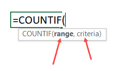
Within the parenthesis, you need to specify the arguments.
In our example, there is only one argument – CellRef.
It’s also a good practice to specify what kind of argument the function expects. In this example, since we will be feeding the function a cell reference, we can specify the argument as a ‘Range’ type. If you don’t specify a data type, VBA would consider it to be a variant (which means you can use any data type).
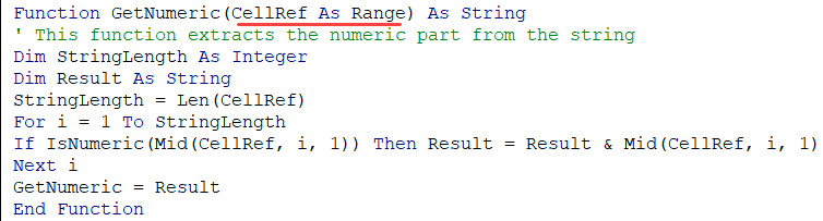
If you have more than one arguments, you can specify those in the same parenthesis – separated by a comma. We will see later in this tutorial on how to use multiple arguments in a user-defined function.
Note that the function is specified as the ‘String’ data type. This would tell VBA that the result of the formula would be of the String data type.
While I can use a numeric data type here (such as Long or Double), doing that would limit the range of numbers it can return. If I have a 20 number long string that I need to extract from the overall string, declaring the function as a Long or Double would give an error (as the number would be out of its range). Hence I have kept the function output data type as String.
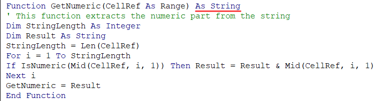
The second line of the code – the one in green that starts with an apostrophe – is a comment. When reading the code, VBA ignores this line. You can use this to add a description or a detail about the code.
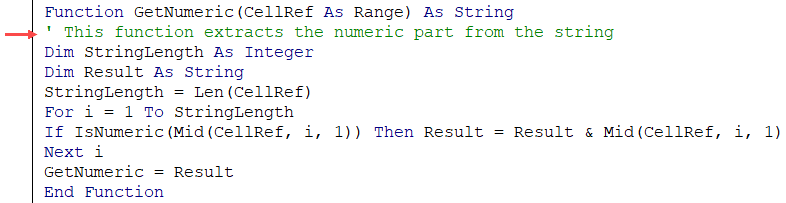
The third line of the code declares a variable ‘StringLength’ as an Integer data type. This is the variable where we store the value of the length of the string that is being analyzed by the formula.
The fourth line declares the variable Result as a String data type. This is the variable where we will extract the numbers from the alphanumeric string.
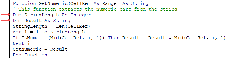
The fifth line assigns the length of the string in the input argument to the ‘StringLength’ variable. Note that ‘CellRef’ refers to the argument that will be given by the user while using the formula in the worksheet (or using it in VBA – which we will see later in this tutorial).
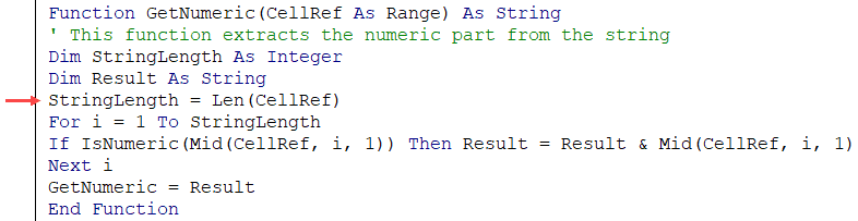
Sixth, seventh, and eighth lines are the part of the For Next loop. The loop runs for as many times as many characters are there in the input argument. This number is given by the LEN function and is assigned to the ‘StringLength’ variable.
So the loop runs from ‘1 to Stringlength’.
Within the loop, the IF statement analyzes each character of the string and if it’s numeric, it adds that numeric character to the Result variable. It uses the MID function in VBA to do this.
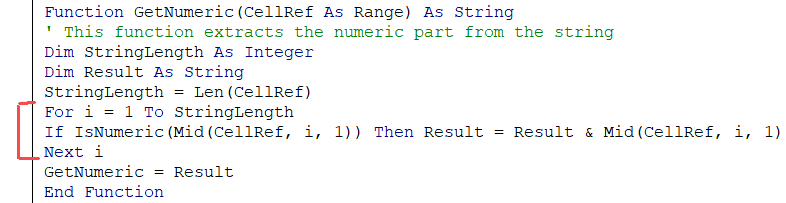
The second last line of the code assigns the value of the result to the function. It’s this line of code that ensures that the function returns the ‘Result’ value back in the cell (from where it’s called).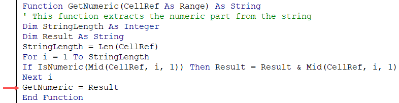
The last line of the code is End Function. This is a mandatory line of code that tells VBA that the function code ends here.
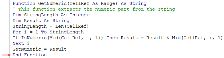
The above code explains the different parts of a typical custom function created in VBA. In the following sections, we will deep dive into these elements and also see the different ways to execute the VBA function in Excel.
Arguments in a User Defined Function in VBA
In the above examples, where we created a user-defined function to get the numeric part from an alphanumeric string (GetNumeric), the function was designed to take one single argument.
In this section, I will cover how to create functions that take no argument to the ones that take multiple arguments (required as well as optional arguments).
Creating a Function in VBA without Any Arguments
In Excel worksheet, we have several functions that take no arguments (such as RAND, TODAY, NOW).
These functions are not dependent on any input arguments. For example, the TODAY function would return the current date and the RAND function would return a random number between 0 and 1.
You can create such similar function in VBA as well.
Below is the code that will give you the name of the file. It doesn’t take any arguments as the result it needs to return is not dependent on any argument.
Function WorkbookName() As String
WorkbookName = ThisWorkbook.Name
End Function
The above code specifies the function’s result as a String data type (as the result we want is the file name – which is a string).
This function assigns the value of ‘ThisWorkbook.Name’ to the function, which is returned when the function is used in the worksheet.
If the file has been saved, it returns the name with the file extension, else it simply gives the name.
The above has one issue though.
If the file name changes, it wouldn’t automatically update. Normally a function refreshes whenever there is a change in the input arguments. But since there are no arguments in this function, the function doesn’t recalculate (even if you change the name of the workbook, close it and then reopen again).
If you want, you can force a recalculation by using the keyboard shortcut – Control + Alt + F9.
To make the formula recalculate whenever there is a change in the worksheet, you need to a line of code to it.
The below code makes the function recalculate whenever there is a change in the worksheet (just like other similar worksheet functions such as TODAY or RAND function).
Function WorkbookName() As String
Application.Volatile True
WorkbookName = ThisWorkbook.Name
End Function
Now, if you change the workbook name, this function would update whenever there is any change in the worksheet or when you reopen this workbook.
Creating a Function in VBA with One Argument
In one of the sections above, we have already seen how to create a function that takes only one argument (the GetNumeric function covered above).
Let’s create another simple function that takes only one argument.
Function created with the below code would convert the referenced text into uppercase. Now we already have a function for it in Excel, and this function is just to show you how it works. If you have to do this, it’s better to use the inbuilt UPPER function.
Function ConvertToUpperCase(CellRef As Range)
ConvertToUpperCase = UCase(CellRef)
End Function
This function uses the UCase function in VBA to change the value of the CellRef variable. It then assigns the value to the function ConvertToUpperCase.
Since this function takes an argument, we don’t need to use the Application.Volatile part here. As soon as the argument changes, the function would automatically update.
Creating a Function in VBA with Multiple Arguments
Just like worksheet functions, you can create functions in VBA that takes multiple arguments.
The below code would create a function that will extract the text before the specified delimiter. It takes two arguments – the cell reference that has the text string, and the delimiter.
Function GetDataBeforeDelimiter(CellRef As Range, Delim As String) as String
Dim Result As String
Dim DelimPosition As Integer
DelimPosition = InStr(1, CellRef, Delim, vbBinaryCompare) - 1
Result = Left(CellRef, DelimPosition)
GetDataBeforeDelimiter = Result
End Function
When you need to use more than one argument in a user-defined function, you can have all the arguments in the parenthesis, separated by a comma.
Note that for each argument, you can specify a data type. In the above example, ‘CellRef’ has been declared as a range datatype and ‘Delim’ has been declared as a String data type. If you don’t specify any data type, VBA considers these are a variant data type.
When you use the above function in the worksheet, you need to give the cell reference that has the text as the first argument and the delimiter character(s) in double quotes as the second argument.
It then checks for the position of the delimiter using the INSTR function in VBA. This position is then used to extract all the characters before the delimiter (using the LEFT function).
Finally, it assigns the result to the function.
This formula is far from perfect. For example, if you enter a delimiter that is not found in the text, it would give an error. Now you can use the IFERROR function in the worksheet to get rid of the errors, or you can use the below code that returns the entire text when it can’t find the delimiter.
Function GetDataBeforeDelimiter(CellRef As Range, Delim As String) as String
Dim Result As String
Dim DelimPosition As Integer
DelimPosition = InStr(1, CellRef, Delim, vbBinaryCompare) - 1
If DelimPosition < 0 Then DelimPosition = Len(CellRef)
Result = Left(CellRef, DelimPosition)
GetDataBeforeDelimiter = Result
End Function
We can further optimize this function.
If you enter the text (from which you want to extract the part before the delimiter) directly in the function, it would give you an error. Go ahead.. try it!
This happens as we have specified the ‘CellRef’ as a range data type.
Or, if you want the delimiter to be in a cell and use the cell reference instead of hard coding it in the formula, you can’t do that with the above code. It’s because the Delim has been declared as a string datatype.
If you want the function to have the flexibility to accept direct text input or cell references from the user, you need to remove the data type declaration. This would end up making the argument as a variant data type, which can take any type of argument and process it.
The below code would do this:
Function GetDataBeforeDelimiter(CellRef, Delim) As String
Dim Result As String
Dim DelimPosition As Integer
DelimPosition = InStr(1, CellRef, Delim, vbBinaryCompare) - 1
If DelimPosition < 0 Then DelimPosition = Len(CellRef)
Result = Left(CellRef, DelimPosition)
GetDataBeforeDelimiter = Result
End Function
Creating a Function in VBA with Optional Arguments
There are many functions in Excel where some of the arguments are optional.
For example, the legendary VLOOKUP function has 3 mandatory arguments and one optional argument.
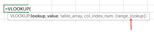
An optional argument, as the name suggests, is optional to specify. If you don’t specify one of the mandatory arguments, your function is going to give you an error, but if you don’t specify the optional argument, your function would work.
But optional arguments are not useless. They allow you to choose from a range of options.
For example, in the VLOOKUP function, if you don’t specify the fourth argument, VLOOKUP does an approximate lookup and if you specify the last argument as FALSE (or 0), then it does an exact match.
Remember that the optional arguments must always come after all the required arguments. You can’t have optional arguments at the beginning.
Now let’s see how to create a function in VBA with optional arguments.
Function with Only an Optional Argument
As far as I know, there is no inbuilt function that takes optional arguments only (I can be wrong here, but I can’t think of any such function).
But we can create one with VBA.
Below is the code of the function that will give you the current date in the dd-mm-yyyy format if you don’t enter any argument (i.e. leave it blank), and in “dd mmmm, yyyy” format if you enter anything as the argument (i.e., anything so that the argument is not blank).
Function CurrDate(Optional fmt As Variant)
Dim Result
If IsMissing(fmt) Then
CurrDate = Format(Date, "dd-mm-yyyy")
Else
CurrDate = Format(Date, "dd mmmm, yyyy")
End If
End Function
Note that the above function uses ‘IsMissing’ to check whether the argument is missing or not. To use the IsMissing function, your optional argument must be of the variant data type.
The above function works no matter what you enter as the argument. In the code, we only check if the optional argument is supplied or not.
You can make this more robust by taking only specific values as arguments and showing an error in rest of the cases (as shown in the below code).
Function CurrDate(Optional fmt As Variant)
Dim Result
If IsMissing(fmt) Then
CurrDate = Format(Date, "dd-mm-yyyy")
ElseIf fmt = 1 Then
CurrDate = Format(Date, "dd mmmm, yyyy")
Else
CurrDate = CVErr(xlErrValue)
End If
End Function
The above code creates a function that shows the date in the “dd-mm-yyyy” format if no argument is supplied, and in “dd mmmm,yyyy” format when the argument is 1. It gives an error in all other cases.
Function with Required as well as Optional Arguments
We have already seen a code that extracts the numeric part from a string.
Now let’s have a look at a similar example that takes both required as well as optional arguments.
The below code creates a function that extracts the text part from a string. If the optional argument is TRUE, it gives the result in uppercase, and if the optional argument is FALSE or is omitted, it gives the result as is.
Function GetText(CellRef As Range, Optional TextCase = False) As String
Dim StringLength As Integer
Dim Result As String
StringLength = Len(CellRef)
For i = 1 To StringLength
If Not (IsNumeric(Mid(CellRef, i, 1))) Then Result = Result & Mid(CellRef, i, 1)
Next i
If TextCase = True Then Result = UCase(Result)
GetText = Result
End Function
Note that in the above code, we have initialized the value of ‘TextCase’ as False (look within the parenthesis in the first line).
By doing this, we have ensured that the optional argument starts with the default value, which is FALSE. If the user specifies the value as TRUE, the function returns the text in upper case, and if the user specifies the optional argument as FALSE or omits it, then the text returned is as is.
Creating a Function in VBA with an Array as the Argument
So far we have seen examples of creating a function with Optional/Required arguments – where these arguments were a single value.
You can also create a function that can take an array as the argument. In Excel worksheet functions, there are many functions that take array arguments, such as SUM, VLOOKUP, SUMIF, COUNTIF, etc.
Below is the code that creates a function that gives the sum of all the even numbers in the specified range of the cells.
Function AddEven(CellRef as Range)
 Dim Cell As Range
 For Each Cell In CellRef
 If IsNumeric(Cell.Value) Then
 If Cell.Value Mod 2 = 0 Then
 Result = Result + Cell.Value
 End If
 End If
 Next Cell
 AddEven = Result
 End Function
You can use this function in the worksheet and provide the range of cells that have the numbers as the argument. The function would return a single value – the sum of all the even numbers (as shown below).
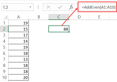
In the above function, instead of a single value, we have supplied an array (A1:A10). For this to work, you need to make sure your data type of the argument can accept an array.
In the code above, I specified the argument CellRef as Range (which can take an array as the input). You can also use the variant data type here.
In the code, there is a For Each loop that goes through each cell and checks if it’s a number of not. If it isn’t, nothing happens and it moves to the next cell. If it’s a number, it checks if it’s even or not (by using the MOD function).
In the end, all the even numbers are added and teh sum is assigned back to the function.
Creating a Function with Indefinite Number of Arguments
While creating some functions in VBA, you may not know the exact number of arguments that a user wants to supply. So the need is to create a function that can accept as many arguments are supplied and use these to return the result.
An example of such worksheet function is the SUM function. You can supply multiple arguments to it (such as this):
=SUM(A1,A2:A4,B1:B20)
The above function would add the values in all these arguments. Also, note that these can be a single cell or an array of cells.
You can create such a function in VBA by having the last argument (or it could be the only argument) as optional. Also, this optional argument should be preceded by the keyword ‘ParamArray’.
‘ParamArray’ is a modifier that allows you to accept as many arguments as you want. Note that using the word ParamArray before an argument makes the argument optional. However, you don’t need to use the word Optional here.
Now let’s create a function that can accept an arbitrary number of arguments and would add all the numbers in the specified arguments:
Function AddArguments(ParamArray arglist() As Variant)
For Each arg In arglist
AddArguments = AddArguments + arg
Next arg
End Function
The above function can take any number of arguments and add these arguments to give the result.
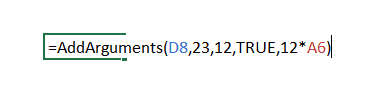
Note that you can only use a single value, a cell reference, a boolean, or an expression as the argument. You can not supply an array as the argument. For example, if one of your arguments is D8:D10, this formula would give you an error.
If you want to be able to use both multi-cell arguments you need to use the below code:
Function AddArguments(ParamArray arglist() As Variant)
For Each arg In arglist
For Each Cell In arg
AddArguments = AddArguments + Cell
Next Cell
Next arg
End Function
Note that this formula works with multiple cells and array references, however, it can not process hardcoded values or expressions. You can create a more robust function by checking and treating these conditions, but that’s not the intent here.
The intent here is to show you how ParamArray works so you can allow an indefinite number of arguments in the function. In case you want a better function than the one created by the above code, use the SUM function in the worksheet.
Creating a Function that Returns an Array
So far we have seen functions that return a single value.
With VBA, you can create a function that returns a variant that can contain an entire array of values.
Array formulas are also available as inbuilt functions in Excel worksheets. If you’re familiar with array formulas in Excel, you would know that these are entered using Control + Shift + Enter (instead of just the Enter). You can read more about array formulas here. If you don’t know about array formulas, don’t worry, keep reading.
Let’s create a formula that returns an array of three numbers (1,2,3).
The below code would do this.
Function ThreeNumbers() As Variant
Dim NumberValue(1 To 3)
NumberValue(1) = 1
NumberValue(2) = 2
NumberValue(3) = 3
ThreeNumbers = NumberValue
End Function
In the above code, we have specified the ‘ThreeNumbers’ function as a variant. This allows it to hold an array of values.
The variable ‘NumberValue’ is declared as an array with 3 elements. It holds the three values and assigns it to the ‘ThreeNumbers’ function.
You can use this function in the worksheet by entering the function and hitting the Control + Shift + Enter key (hold the Control and the Shift keys and then press Enter).
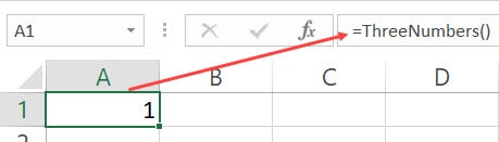
When you do this, it will return 1 in the cell, but in reality, it holds all the three values. To check this, use the below formula:
=MAX(ThreeNumbers())
Use the above function with Control + Shift + Enter. You will notice that the result is now 3, as it is the largest values in the array returned by the Max function, which gets the three numbers as the result of our user-defined function – ThreeNumbers.
You can use the same technique to create a function that returns an array of Month Names as shown by the below code:
Function Months() As Variant
Dim MonthName(1 To 12)
MonthName(1) = "January"
MonthName(2) = "February"
MonthName(3) = "March"
MonthName(4) = "April"
MonthName(5) = "May"
MonthName(6) = "June"
MonthName(7) = "July"
MonthName(8) = "August"
MonthName(9) = "September"
MonthName(10) = "October"
MonthName(11) = "November"
MonthName(12) = "December"
Months = MonthName
End Function
Now when you enter the function =Months() in Excel worksheet and use Control + Shift + Enter, it will return the entire array of month names. Note that you see only January in the cell as that is the first value in the array. This does not mean that the array is only returning one value.
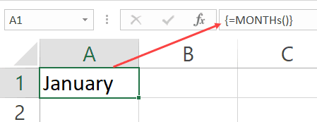
To show you the fact that it is returning all the values, do this – select the cell with the formula, go to the formula bar, select the entire formula and press F9. This will show you all the values that the function returns.

You can use this by using the below INDEX formula to get a list of all the month names in one go.
=INDEX(Months(),ROW())
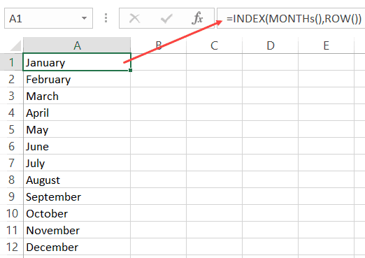
Now if you have a lot of values, it’s not a good practice to assign these values one by one (as we have done above). Instead, you can use the Array function in VBA.
So the same code where we create the ‘Months’ function would become shorter as shown below:
Function Months() As Variant
Months = Array("January", "February", "March", "April", "May", "June", _
"July", "August", "September", "October", "November", "December")
End Function
The above function uses the Array function to assign the values directly to the function.
Note that all the functions created above return a horizontal array of values. This means that if you select 12 horizontal cells (let’s say A1:L1), and enter the =Months() formula in cell A1, it will give you all the month names.
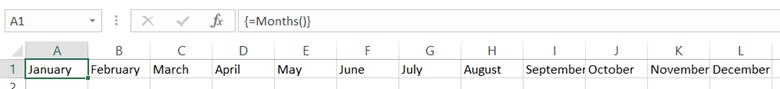
But what if you want these values in a vertical range of cells.
You can do this by using the TRANSPOSE formula in the worksheet.
Simply select 12 vertical cells (contiguous), and enter the below formula.
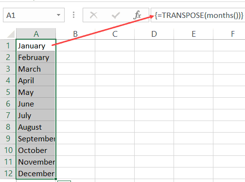
Understanding the Scope of a User Defined Function in Excel
A function can have two scopes – Public or Private.
- A Public scope means that the function is available for all the sheets in the workbook as well as all the procedures (Sub and Function) across all modules in the workbook. This is useful when you want to call a function from a subroutine (we will see how this is done in the next section).
- A Private scope means that the function is available only in the module in which it exists. You can’t use it in other modules. You also won’t see it in the list of functions in the worksheet. For example, if your Function name is ‘Months()’, and you type function in Excel (after the = sign), it will not show you the function name. You can, however, still, use it if you enter the formula name.
If you don’t specify anything, the function is a Public function by default.
Below is a function that is a Private function:
Private Function WorkbookName() As String
WorkbookName = ThisWorkbook.Name
End Function
You can use this function in the subroutines and the procedures in the same modules, but can’t use it in other modules. This function would also not show up in the worksheet.
The below code would make this function Public. It will also show up in the worksheet.
Function WorkbookName() As String
WorkbookName = ThisWorkbook.Name
End Function
Different Ways of Using a User Defined Function in Excel
Once you have created a user-defined function in VBA, you can use it in many different ways.
Let’s first cover how to use the functions in the worksheet.
Using UDFs in Worksheets
We have already seen examples of using a function created in VBA in the worksheet.
All you need to do is enter the functions name, and it shows up in the intellisense.
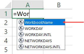
Note that for the function to show up in the worksheet, it must be a Public function (as explained in the section above).
You can also use the Insert Function dialog box to insert the user defined function (using the steps below). This would work only for functions that are Public.
The above steps would insert the function in the worksheet. It also displays a Function Arguments dialog box that will give you details on the arguments and the result.
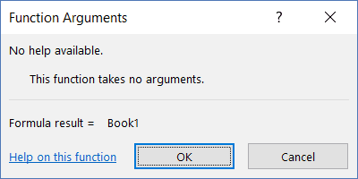
You can use a user defined function just like any other function in Excel. This also means that you can use it with other inbuilt Excel functions. For example. the below formula would give the name of the workbook in upper case:
=UPPER(WorkbookName())
Using User Defined Functions in VBA Procedures and Functions
When you have created a function, you can use it in other sub-procedures as well.
If the function is Public, it can be used in any procedure in the same or different module. If it’s Private, it can only be used in the same module.
Below is a function that returns the name of the workbook.
Function WorkbookName() As String
WorkbookName = ThisWorkbook.Name
End Function
The below procedure call the function and then display the name in a message box.
Sub ShowWorkbookName()
MsgBox WorkbookName
End Sub
You can also call a function from another function.
In the below codes, the first code returns the name of the workbook, and the second one returns the name in uppercase by calling the first function.
Function WorkbookName() As String
WorkbookName = ThisWorkbook.Name
End Function
Function WorkbookNameinUpper()
WorkbookNameinUpper = UCase(WorkbookName)
End Function
Calling a User Defined Function from Other Workbooks
If you have a function in a workbook, you can call this function in other workbooks as well.
There are multiple ways to do this:
- Creating an Add-in
- Saving function in the Personal Macro Workbook
- Referencing the function from another workbook.
Creating an Add-in
By creating and installing an add-in, you will have the custom function in it available in all the workbooks.
Suppose you have created a custom function – ‘GetNumeric’ and you want it in all the workbooks. To do this, create a new workbook and have the function code in a module in this new workbook.
Now follow the steps below to save it as an add-in and then install it in Excel.
Now the add-in has been activated.
Now you can use the custom function in all the workbooks.
Saving the Function in Personal Macro Workbook
A Personal Macro Workbook is a hidden workbook in your system that opens whenever you open the Excel application.
It’s a place where you can store macro codes and then access these macros from any workbook. It’s a great place to store those macros that you want to use often.
By default, there is no personal macro workbook in your Excel. You need to create it by recording a macro and saving it in the Personal macro workbook.
You can find the detailed steps on how to create and save macros in the personal macro workbook here.
Referencing the function from another workbook
While the first two methods (creating an add-in and using personal macro workbook) would work in all situations, if you want to reference the function from another workbook, that workbook needs to be open.
Suppose you have a workbook with the name ‘Workbook with Formula’, and it has the function with the name ‘GetNumeric’.
To use this function in another workbook (while the Workbook with Formula is open), you can use the below formula:
=’Workbook with Formula’!GetNumeric(A1)
The above formula will use the user defined function in the Workbook with Formula file and give you the result.
Note that since the workbook name has spaces, you need to enclose it in single quotes.
Using Exit Function Statement VBA
If you want to exit a function while the code is running, you can do that by using the ‘Exit Function’ statement.
The below code would extract the first three numeric characters from an alphanumeric text string. As soon as it gets the three characters, the function ends and returns the result.
Function GetNumericFirstThree(CellRef As Range) As Long
Dim StringLength As Integer
StringLength = Len(CellRef)
For i = 1 To StringLength
If J = 3 Then Exit Function
If IsNumeric(Mid(CellRef, i, 1)) Then
J = J + 1
Result = Result & Mid(CellRef, i, 1)
GetNumericFirstThree = Result
End If
Next i
End Function
The above function checks for the number of characters that are numeric, and when it gets 3 numeric characters, it Exits the function in the next loop.
Debugging a User Defined Function
There are a few techniques you can use while debugging a user-defined function in VBA:
Debugging a Custom Function by Using the Message Box
Use MsgBox function to show a message box with a specific value.
The value you display can be based on what you want to test. For example, if you want to check if the code is getting executed or not, any message would work, and if you want to check whether the loops are working or not, you can display a specific value or the loop counter.
Debugging a Custom Function by Setting the Breakpoint
Set a breakpoint to be able to go step through each line one at a time. To set a breakpoint, select the line where you want it and press F9, or click on the gray vertical area which is left to the code lines. Any of these methods would insert a breakpoint (you will see a red dot in the gray area).
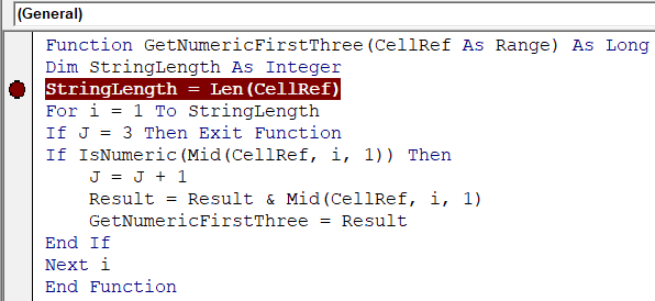
Once you have set the breakpoint and you execute the function, it goes till the breakpoint line and then stops. Now you can step through the code using the F8 key. Pressing F8 once moves to the next line in the code.
Debugging a Custom Function by Using Debug.Print in the Code
You can use Debug.Print statement in your code to get the values of the specified variables/arguments in the immediate window.
For example, in the below code, I have used Debug.Print to get the value of two variables – ‘j’ and ‘Result’
Function GetNumericFirstThree(CellRef As Range) As Long
Dim StringLength As Integer
StringLength = Len(CellRef)
For i = 1 To StringLength
If J = 3 Then Exit Function
If IsNumeric(Mid(CellRef, i, 1)) Then
 J = J + 1
 Result = Result & Mid(CellRef, i, 1)
 Debug.Print J, Result
 GetNumericFirstThree = Result
End If
Next i
End Function
When this code is executed, it shows the following in the immediate window.
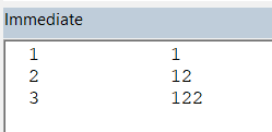
Excel Inbuilt Functions Vs. VBA User Defined Function
There are few strong benefits of using Excel in-built functions over custom functions created in VBA.
- Inbuilt functions are a lot faster than the VBA functions.
- When you create a report/dashboard using VBA functions, and you send it to a client/colleague, they wouldn’t have to worry about whether the macros are enabled or not. In some cases, clients/customers get scared by seeing a warning in the yellow bar (which simply asks them to enable macros).
- With inbuilt Excel functions, you don’t need to worry about file extensions. If you have macros or user-defined functions in the workbook, you need to save it in .xlsm.
While there are many strong reasons to use Excel in-built functions, in a few cases, you’re better off using a user-defined function.
- It’s better to use a user-defined function if your inbuilt formula is huge and complicated. This becomes even more relevant when you need someone else to update the formulas. For example, if you have a huge formula made up of many different functions, even changing a reference to a cell can be tedious and error-prone. Instead, you can create a custom function that only takes one or two arguments and does all the heavy lifting the backend.
- When you have to get something done that can not be done by Excel inbuilt functions. An example of this can be when you want to extract all the numeric characters from a string. In such cases, the benefit of using a user-defined function gar outweighs its negatives.
Where to put the VBA Code for a User-Defined Function
When creating a custom function, you need to put the code in the code window for the workbook in which you want the function.
Below are the steps to put the code for the ‘GetNumeric’ function in the workbook.
- Go to the Developer tab.

- Click on the Visual Basic option. This will open the VB editor in the backend.
- In the Project Explorer pane in the VB Editor, right-click on any object for the workbook in which you want to insert the code. If you don’t see the Project Explorer go to the View tab and click on Project Explorer.
- Go to Insert and click on Module. This will insert a module object for your workbook.

- Copy and paste the code in the module window.

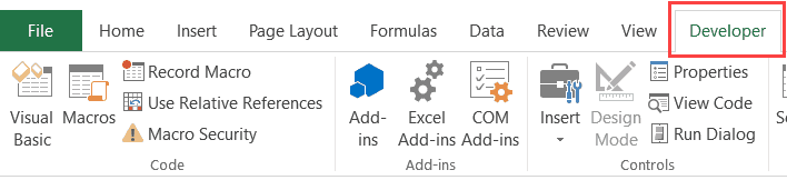
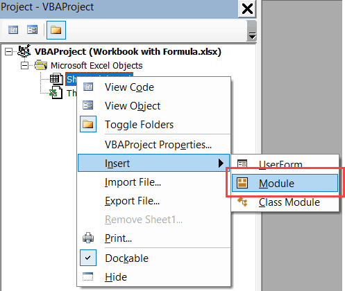
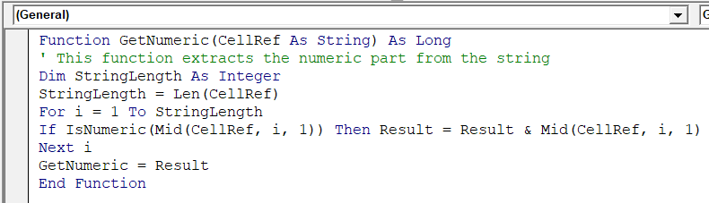
You May Also Like the Following Excel VBA Tutorials:
- Working with Cells and Ranges in Excel VBA.
- Working with Worksheets in Excel VBA.
- Working with Workbooks using VBA.
- How to use Loops in Excel VBA.
- Excel VBA Events – An Easy (and Complete) Guide
- Using IF Then Else Statements in VBA.
- How to Record a Macro in Excel.
- How to Run a Macro in Excel.
- How to Sort Data in Excel using VBA (A Step-by-Step Guide).
- Excel VBA InStr Function – Explained with Examples.
Создание пользовательской функции в VBA Excel, ее синтаксис и компоненты. Описание пользовательской функции и ее аргументов. Метод Application.MacroOptions.
Пользовательская функция — это процедура VBA, которая производит заданные вычисления и возвращает полученный результат. Используется для вставки в ячейки рабочего листа Excel или для вызова из других процедур.
Объявление пользовательской функции
Синтаксис функции
|
[Static] Function Имя ([СписокАргументов])[As ТипДанных] [Операторы] [Имя = выражение] [Exit Function] [Операторы] [Имя = выражение] End Function |
Компоненты функции
- Static — необязательное ключевое слово, указывающее на то, что значения переменных, объявленных в функции, сохраняются между ее вызовами.
- Имя — обязательный компонент, имя пользовательской функции.
- СписокАргументов — необязательный компонент, одна или более переменных, представляющих аргументы, которые передаются в функцию. Аргументы заключаются в скобки и разделяются между собой запятыми.
- Операторы — необязательный компонент, блок операторов (инструкций).
- Имя = выражение — необязательный* компонент, присвоение имени функции значения выражения или переменной. Обычно, значение присваивается функции непосредственно перед выходом из нее.
- Exit Function — необязательный компонент, принудительный выход из функции, если ей уже присвоено окончательное значение.
*Один из компонентов Имя = выражение следует считать обязательным, так как если не присвоить функции значения, смысл ее использования теряется.
Видимость функции
Видимость пользовательской функции определяется необязательными ключевыми словами Public и Private, которые могут быть указаны перед оператором Function (или Static, в случае его использования).
Ключевое слово Public указывает на то, что функция будет доступна для вызова из других процедур во всех модулях открытых книг Excel. Функция, объявленная как Public, отображается в диалоговом окне Мастера функций.
Ключевое слово Private указывает на то, что функция будет доступна для вызова из других процедур только в пределах программного модуля, в котором она находится. Функция, объявленная как Private, не отображается в диалоговом окне Мастера функций, но ее можно ввести в ячейку вручную.
Если ключевое слово Public или Private не указано, функция считается по умолчанию объявленной, как Public.
Чтобы пользовательская функция всегда была доступна во всех открытых книгах Excel, сохраните ее в Личной книге макросов без объявления видимости или как Public. Но если вы планируете передать рабочую книгу с пользовательской функцией на другой компьютер, код функции должен быть в программном модуле передаваемой книги.
Пример пользовательской функции
Для примера мы рассмотрим простейшую пользовательскую функцию, которой в следующем параграфе добавим описание. Называется функция «Деление», объявлена с типом данных Variant, так как ее возвращаемое значение может быть и числом, и текстом. Аргументы функции — Делимое и Делитель — тоже объявлены как Variant, так как в ячейках Excel могут быть числовые значения разных типов, и функция IsNumeric тоже проверяет разные типы данных и требует, чтобы ее аргументы были объявлены как Variant.
|
Function Деление(Делимое As Variant, Делитель As Variant) As Variant If IsNumeric(Делимое) = False Or IsNumeric(Делитель) = False Then Деление = «Ошибка: Делимое и Делитель должны быть числами!» Exit Function ElseIf Делитель = 0 Then Деление = «Ошибка: деление на ноль!» Exit Function Else Деление = Делимое / Делитель End If End Function |
Эта функция выполняет деление значений двух ячеек рабочего листа Excel. Перед делением проверяются два блока условий:
- Если делимое или делитель не являются числом, функция возвращает значение: «Ошибка: Делимое и Делитель должны быть числами!», и производится принудительный выход из функции оператором Exit Function.
- Если делитель равен нулю, функция возвращает значение: «Ошибка: деление на ноль!», и производится принудительный выход из функции оператором Exit Function.
Если проверяемые условия не выполняются (возвращают значение False) производится деление чисел и функция возвращает частное (результат деления).
Вы можете скопировать к себе в стандартный модуль эту функцию и она станет доступна в разделе «Определенные пользователем» Мастера функций. Попробуйте вставить функцию «Деление» в ячейку рабочего листа с помощью Мастера и поэкспериментируйте с ней.
Практического смысла функция «Деление» не имеет, но она хорошо демонстрирует как объявляются, создаются и работают пользовательские функции в VBA Excel. А еще она поможет продемонстрировать, как добавлять к функциям и аргументам описания. С полноценной пользовательской функцией вы можете ознакомиться здесь.
Добавление описания функции
В списке функций, выводимом Мастером, невозможно добавить или отредактировать их описание. Список макросов позволяет добавлять процедурам описание, но в нем нет функций. Проблема решается следующим образом:
- Запустите Мастер функций, посмотрите, как отображается имя нужной функции и закройте его.
- Откройте список макросов и в поле «Имя макроса» впишите имя пользовательской функции.
- Нажмите кнопку «Параметры» и в открывшемся окне добавьте или отредактируйте описание.
- Нажмите кнопку «OK», затем в окне списка макросов — «Отмена». Описание готово!
Добавление описания на примере функции «Деление»:

Добавление описания пользовательской функции
Описание функции «Деление» в диалоговом окне Мастера функций «Аргументы функции»:

Описание пользовательской функции в окне «Аргументы функции»
С помощью окна «Список макросов» можно добавить описание самой функции, а ее аргументам нельзя. Но это можно сделать, используя метод Application.MacroOptions.
Метод Application.MacroOptions
Метод Application.MacroOptions позволяет добавить пользовательской функции описание, назначить сочетание клавиш, указать категорию, добавить описания аргументов и добавить или изменить другие параметры. Давайте рассмотрим возможности этого метода, используемые чаще всего.
Пример кода с методом Application.MacroOptions:
|
Sub ИмяПодпрограммы() Application.MacroOptions _ Macro:=«ИмяФункции», _ Description:=«Описание функции», _ Category:=«Название категории», _ ArgumentDescriptions:=Array(«Описание 1», «Описание 2», «Описание 3», ...) End Sub |
- ИмяПодпрограммы — любое уникальное имя, подходящее для наименования процедур.
- ИмяФункции — имя функции, параметры которой добавляются или изменяются.
- Описание функции — описание функции, которое добавляется или изменяется.
- Название категории — название категории в которую будет помещена функция. Если параметр Category отсутствует, пользовательская функция будет записана в раздел по умолчанию — «Определенные пользователем». Если указанное Название категории соответствует одному из названий стандартного списка, функция будет записана в него. Если такого Названия категории нет в списке, будет создан новый раздел с этим названием и функция будет помещена в него.
- «Описание 1», «Описание 2», «Описание 3», … — описания аргументов в том порядке, как они расположены в объявлении пользовательской функции.
Эта подпрограмма запускается один раз, после чего ее можно удалить или использовать как шаблон для корректировки параметров других пользовательских функций.
Сейчас с помощью метода Application.MacroOptions попробуем изменить описание пользовательской функции «Деление» и добавить описания аргументов.
|
Sub ИзменениеОписания() Application.MacroOptions _ Macro:=«Деление», _ Description:=«Описание функции Деление изменено методом Application.MacroOptions», _ ArgumentDescriptions:=Array(«- любое числовое значение», «- числовое значение, кроме нуля») End Sub |
После однократного запуска этой подпрограммы получаем следующий результат:

Новое описание пользовательской функции и ее второго аргумента
Метод Application.MacroOptions не работает в Личной книге макросов, но и здесь можно найти решение. Добавьте описания к пользовательским функциям и их аргументам в обычной книге Excel, затем экспортируйте модуль с функциями в любой каталог на жестком диске и оттуда импортируйте в Личную книгу макросов. Все описания сохранятся.
In this Article
- Creating a Function without Arguments
- Calling a Function from a Sub Procedure
- Creating Functions
- Single Argument
- Multiple Arguments
- Optional Arguments
- Default Argument Value
- ByVal and ByRef
- Exit Function
- Using a Function from within an Excel Sheet
This tutorial will teach you to create and use functions with and without parameters in VBA
VBA contains a large amount of built-in functions for you to use, but you are also able to write your own. When you write code in VBA, you can write it in a Sub Procedure, or a Function Procedure. A Function Procedure is able to return a value to your code. This is extremely useful if you want VBA to perform a task to return a result. VBA functions can also be called from inside Excel, just like Excel’s built-in Excel functions.
Creating a Function without Arguments
To create a function you need to define the function by giving the function a name. The function can then be defined as a data type indicating the type of data you want the function to return.
You may want to create a function that returns a static value each time it is called – a bit like a constant.
Function GetValue() As Integer
   GetValue = 50
End Function
If you were to run the function, the function would always return the value of 50.
You can also create functions that refer to objects in VBA but you need to use the Set Keyword to return the value from the function.
Function GetRange() as Range
  Set GetRange = Range("A1:G4")
End Function
If you were to use the above function in your VBA code, the function would always return the range of cells A1 to G4 in whichever sheet you are working in.
Calling a Function from a Sub Procedure
Once you create a function, you can call it from anywhere else in your code by using a Sub Procedure to call the function.
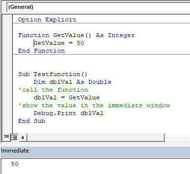
The value of 50 would always be returned.
You can also call the GetRange function from a Sub Procedure.
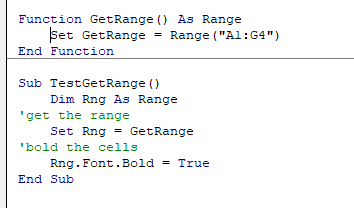
In the above example, the GetRange Function is called by the Sub Procedure to bold the cells in the range object.
Creating Functions
Single Argument
You can also assign a parameter or parameters to your function. These parameters can be referred to as Arguments.
Function ConvertKilosToPounds (dblKilo as Double) as Double
   ConvertKiloToPounds = dblKilo*2.2
End Function
We can then call the above function from a Sub Procedure in order to work out how many pounds a specific amount of kilos are.
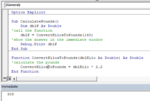
A function can be a called from multiple procedures within your VBA code if required. This is very useful in that it stops you from having to write the same code over and over again. It also enables you to divide long procedures into small manageable functions.
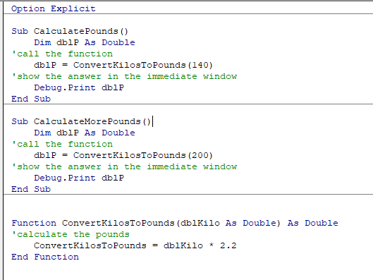
In the above example, we have 2 procedures – each of them are using the Function to calculate the pound value of the kilos passed to them in the dblKilo Argument of the function.
Multiple Arguments
You can create a Function with multiple arguments and pass the values to the Function by way of a Sub Procedure.
Function CalculateDayDiff(Date1 as Date, Date2 as Date) as Double
   CalculateDayDiff = Date2-Date1
End Function
We can then call the function to calculate the amount of days between 2 dates.
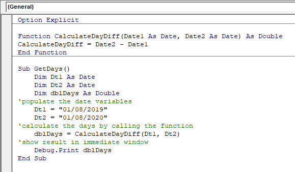
Optional Arguments
You can also pass Optional arguments to a Function. In other words, sometimes you may need the argument, and sometimes you may not – depending on what code you are using the Function with .
Function CalculateDayDiff(Date1 as Date, Optional Date2 as Date) as Double
'check for second date and if not there, make Date2 equal to today's date.
   If Date2=0 then Date2 = Date
'calculate difference
   CalculateDayDiff = Date2-Date1
End Function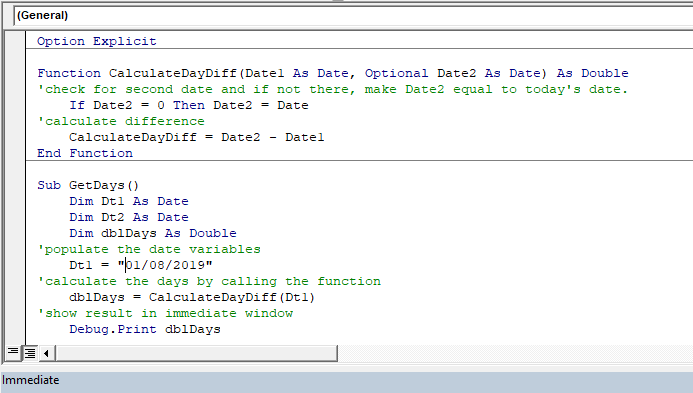
VBA Coding Made Easy
Stop searching for VBA code online. Learn more about AutoMacro — A VBA Code Builder that allows beginners to code procedures from scratch with minimal coding knowledge and with many time-saving features for all users!

Learn More
Default Argument Value
You can also set the default value of the Optional arguments when you are creating the function so that if the user omits the argument, the value that you have put as default will be used instead.
Function CalculateDayDiff(Date1 as Date, Optional Date2 as Date="06/02/2020") as Double
'calculate difference
   CalculateDayDiff = Date2-Date1
End Function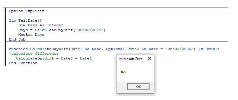
ByVal and ByRef
When you pass values to a function, you can use the ByVal or ByRef keywords. If you omit either of these, the ByRef is used as the default.
ByVal means that you are passing a copy of the variable to the function, whereas ByRef means you are referring to the original value of the variable. When you pass a copy of the variable (ByVal), the original value of the variable is NOT changed, but when you reference the variable, the original value of the variable is changed by the function.
Function GetValue(ByRef intA As Integer) As Integer
   intA = intA * 4
   GetValue = intA
End Function
In the function above, the ByRef could be omitted and the function would work the same way.
Function GetValue(intA As Integer) As Integer
   intA = intA * 4
   GetValue = intA
End Function
To call this function, we can run a sub-procedure.
Sub TestValues()
   Dim intVal As Integer
'populate the variable with the value 10
   intVal = 10
'run the GetValue function, and show the value in the immediate window
   Debug.Print GetValue(intVal)
'show the value of the intVal variable in the immediate window
   Debug.Print  intVal
End Sub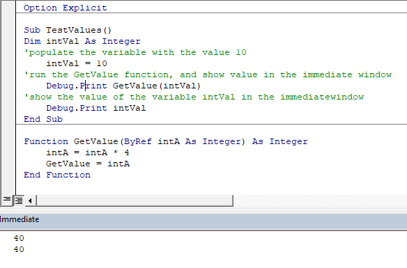
Note that the debug windows show the value 40 both times. When you pass the variable IntVal to the function – the value of 10 is passed to the function, and multiplied by 4. Using the ByRef keyword (or omitting it altogether), will AMEND the value of the IntVal variable. This is shown when you show first the result of the function in the immediate window (40), and then the value of the IntVal variable in the debug window (also 40).
If we do NOT want to change the value of the original variable, we have to use ByVal in the function.
Function GetValue(ByVal intA As Integer) As Integer
intA = intA * 4
GetValue = intA
End Function
Now if we call the function from a sub-procedure, the value of the variable IntVal will remain at 10.
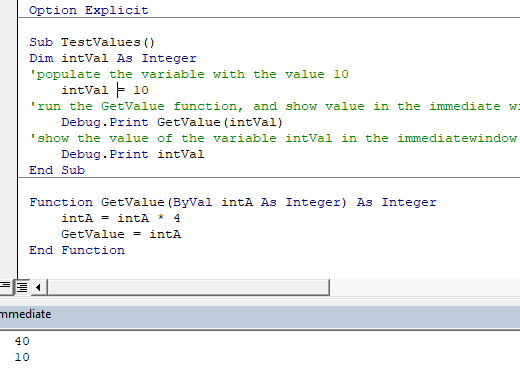
Exit Function
If you create a function that tests for a certain condition, and once the condition is found to be true, you want return the value from the function, you may need to add an Exit Function statement in your Function in order to exit the function before you have run through all the code in that function.
Function FindNumber(strSearch As String) As Integer
   Dim i As Integer
'loop through each letter in the string
   For i = 1 To Len(strSearch)
   'if the letter is numeric, return the value to the function
      If IsNumeric(Mid(strSearch, i, 1)) Then
         FindNumber= Mid(strSearch, i, 1)
   'then exit the function
         Exit Function
      End If
   Next
   FindNumber= 0
End Function
The function above will loop through the string that is provided until it finds a number, and then return that number from the string. It will only find the first number in the string as it will then Exit the function.
The function above can be called by a Sub routine such as the one below.
Sub CheckForNumber()
   Dim NumIs as Integer
'pass a text string to the find number function
   NumIs = FindNumber("Upper Floor, 8 Oak Lane, Texas")
'show the result in the immediate window
   Debug.Print NumIs
End Sub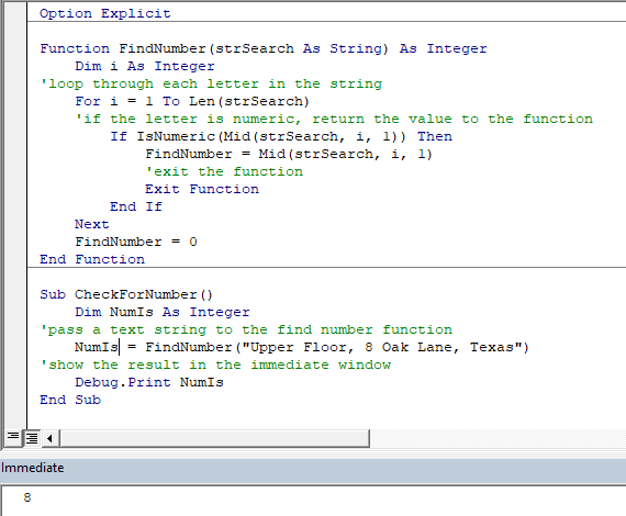
VBA Programming | Code Generator does work for you!
Using a Function from within an Excel Sheet
In addition to calling a function from your VBA code using a sub procedure, you can also call the function from within your Excel sheet. The functions that you have created should by default appear in your function list in the User Defined section of the function list.
Click on the fx to show the Insert Function dialog box.
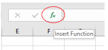
Select User Defined from the Category List
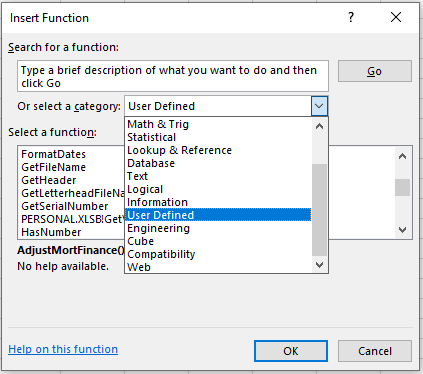
Select the function you require from the available User Defined Functions (UDF’s).

Alternatively, when you start writing your function in Excel, the function should appear in the drop down list of functions.
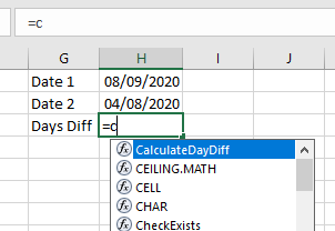
If you do not want the function to be available inside an Excel sheet, you need to put the Private word in front of the word Function when you create the function in your VBA code.
Private Function CalculateDayDiff(Date1 as Date, Date2 as Date) as Double
   CalculateDayDiff = Date2-Date1
End Function
It will now not appear in the drop down list showing the Excel functions available.
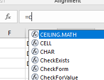
Interestingly enough, however, you can still use the function – it just will not appear in the list when looking for it!
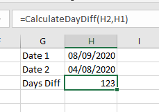
If you have declared the second argument as Optional, you can omit it within the Excel sheet as well as within the VBA code.
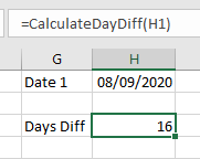
You can also use the a function that you have created without arguments in your Excel sheet.
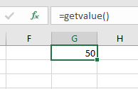
") One of the most commonly used features in Excel are its functions.
One of the most commonly used features in Excel are its functions.
This is hardly surprising. After all, Excel has hundreds of built-in functions.
The variety, in terms of uses and complexity, is quite remarkable. Excel seems to have a function for everything.
But…
Is this really the case?
And…
Even assuming that there is a function for everything, is relying solely on Excel’s built-in functions the most productive way to work?
If these type of questions have ever crossed your mind, and you’ve ever wondered how you can create new functions in Excel, I’m sure you’ll find this tutorial interesting.
On the other hand, you may think that with all the functions that are available in Excel, there is absolutely no need to create new functions. If that is the case, I’m confident that you’ll still find useful information in this blog post. Additionally, I believe that the information within it may just change your opinion.
The reason why I believe that, regardless of your opinion about the need to create new functions in Excel, you’ll find this Excel tutorial interesting is that, indeed, it explains how to you can create your own custom functions (technically called VBA Function procedures). And, just in case you believe this is unnecessary, this guide also provides strong reasons why you should consider creating and using these custom VBA functions.
The main purpose of this tutorial is to introduce to you Excel VBA Function procedures, also known as custom functions, User-Defined Functions or UDFs. More precisely, after reading this Excel tutorial on Excel VBA Function procedures, you’ll know the most relevant aspects regarding the following topics:
Where relevant, every concept and explanation is illustrated with the help of a basic example.
This Excel VBA Function Procedures Tutorial is accompanied by an Excel workbook containing these examples. You can get immediate free access to this example workbook by subscribing to the Power Spreadsheets Newsletter.
Let’s start by understanding, more precisely…
What Is A Procedure: Excel VBA Function Procedures Vs. VBA Sub Procedures
In general terms, a procedure is the part of a computer program that performs a particular task or action. If you’re working with Excel’s Visual Basic Editor, a procedure is the block of statements enclosed by a declaration statement and an End declaration.
When working with Visual Basic for Applications, you’ll constantly encounter 2 types of procedures:
- Sub procedures, which carry out one or more actions in Excel.
- Sub procedures don’t require arguments and don’t return data. You’ll see below that Function procedures do both of these.
- Function procedures, which carry out a calculation and return a value (can be a number or a string) or array.
- Function procedures are passive: they generally don’t carry out any actions. There is, however, at least one exception to this rule: It is possible to change the text in a cell comment using Function procedures.
- There are other methods that, when used in a VBA function, can also make changes to a workbook. Additionally, Function procedures that aren’t used in worksheet formulas can do pretty much the same as a regular Sub procedure.
In practice, you’re likely to (mostly) work with Sub procedures. In other words: Most of the procedures you’ll create will (likely) be Sub procedures.
The reason for this is that most macros are small/brief automations. As a consequence, most macros are self-contained Sub procedures.
The fact that most macros are self-contained Sub procedures used to carry out relatively simple jobs shouldn’t stop you from creating more complex and sophisticated macros when required.
As you’ll see in this Excel tutorial, VBA Function procedures can play a key role when creating complex and sophisticated macros. Therefore, let’s take a closer look at…
What Is An Excel VBA Function Procedure
Even if you’re not very familiar with Excel, you’re probably familiar with the concept of functions.
The reason for this is that, even if you’ve never used Visual Basic for Applications, you’ve probably worked quite a bit with worksheet functions. These are the functions that you use every time you create a formula in an Excel worksheet and, as a side-note, you can also use them in VBA.
Some examples of worksheet functions are SUM, IF, IFERROR and VLOOKUP function.
Worksheet functions work very similarly to Excel VBA Function procedures. Worksheet functions (generally) proceed as follows:
- Step #1: They generally take one or more arguments. There are some exceptions to this rule, as some functions such as TRUE and FALSE take no arguments.
- Step #2: The functions carry out a particular calculation.
- Step #3: Finally, a value is returned.
Excel VBA Function procedures do exactly the same thing. In other words, VBA functions take arguments and return values.
VBA Function procedures are very versatile. You can use them both when working with Visual Basic for Applications or directly in an Excel worksheet formula. I explain both ways of executing a VBA Function procedure below.
If Excel VBA Function procedures function similarly to regular worksheet functions, you may wonder…
Why Create And Use Excel VBA Function Procedures?
Excel has hundreds of functions. These functions carry out a huge range of calculations, some more useful than others.
Considering the huge amount of available worksheet functions, you may wonder whether you should take the time to learn how to create additional functions using Visual Basic for Applications.
I hope that, after reading this Excel tutorial and getting an idea about what Excel VBA Function procedures can do for you, you’ll agree with me that it makes sense to learn about this tool and use it when appropriate. The reason is that VBA Function procedures allow you to simplify your work. More precisely: User-Defined Functions (Function procedures) are useful when working with both:
- Worksheet formulas; and
- VBA procedures.
The following are some of the advantages of using Excel VBA Function procedures:
- VBA Function procedures can help you shorten your formulas. Shorter formulas are easier to read and understand. More generally, they are easier to work with.
- When creating applications, custom functions may help you reduce duplicated code. Among other advantages, this helps you minimize errors.
- When using VBA functions, you can write functions that perform operations that would (otherwise) be impossible.
The simplicity of of Excel VBA Function procedures (once they’re created) is illustrated by the fact that, once the User-Defined Function (Function procedure) has been created, a regular user (only) needs to know the function’s:
- Name; and
- Arguments.
VBA Function procedures can be extremely helpful when creating large and complex VBA projects. The reason for this is that, when working in large projects, you’ll usually create a structure involving multiple procedures (both Sub and Function procedures).
Since VBA Functions take incoming data (arguments) and return other data (values that result from calculations), they’re very useful for purposes of helping different procedures communicate between themselves. In other words, one of the strongest reasons why you should create and use VBA Function procedures is for purposes of improving your VBA coding skills in general. Appropriately working with Function procedures and Sub procedures becomes increasingly important as the size and complexity of your VBA Applications increases.
More precisely, when creating large and complex projects, you can take advantage of the ability of VBA functions to return a value. You can (usually) do this by assigning the name of the Excel VBA Function procedure to a variable in the section of the procedure where you call the function.
I explain how to call VBA Function procedures from other procedures further below.
Basic Syntax Of An Excel VBA Function Procedure
When working with VBA Sub procedures you can, up to a certain extent, rely on Excel’s macro recorder. This allows you to create basic macros by simply carrying out and recording the actions you want the macro to record and store.
When working with Excel VBA Function procedures, you can’t use the macro recorder. In other words, you must always enter the relevant VBA code.
The macro recorder may, however, be a helpful tool for purposes of finding properties (which I explain this blog post) and methods (which I cover here) that you may want to use in the Function procedure you’re creating.
The basic elements of an Excel VBA Function procedure are the following:
- It always begins with the Function keyword.
- It always ends with the End Function statement.
- Between the declaration and End statements, it contains the relevant block of statements with instructions.
As an example, let’s take the following very simple Excel VBA Function procedure (called Squared), which simply squares a certain number which is given to it as an argument.

In practice, you’ll be working with much more complex VBA Function procedures. However, this basic function is enough for the purposes of this Excel tutorial and allows us to focus in understanding the concepts that will later allow you to build much more complicated Function procedures.
Let’s take a closer look at the first element of the sample Excel VBA Function above:
Declaration Statement Of An Excel VBA Function Procedure
As you can see in the example above, the first statement is composed of 3 items:
- The Function keyword, which declares the beginning of the VBA Function procedure.

- The name of the VBA Function procedure which, in this example, is “Squared”.
- The arguments taken by the VBA function, enclosed by parentheses. In the example above, the Squared function takes only 1 argument: number.
- If the VBA Function procedure that you’re creating takes several arguments, use a comma (,) to separate them.
- If you’re creating a function that takes no arguments, leave the parentheses empty. Note that you must always have the parentheses, even if they are empty.
- I explain the concept of arguments, in the context of Excel VBA Function procedures, in more detail below.
How To Name Excel VBA Function Procedures
The name of the VBA Function procedure appears in the declaration statement itself, as shown above.
As a general rule, Function procedure names must follow the sale rules as variable names. These rules are substantially the same as those that apply to naming naming VBA Sub procedures and, more generally, to most items or elements within the Visual Basic for Applications environment.
The following are the main rules when naming variables:
- Names must start with letters.
- As long as the name complies with the above, they can also include numbers and certain (not all) punctuation characters. For example, underscore (_) is commonly used.
- The maximum number of characters a name can have is 255.
- Names can’t be the same as any of Excel’s key words, such as “Sheet”.
- No spaces are allowed. In other words, names must be a “continuous string of characters only”.
The following are common additional suggestions for naming your VBA Function procedures:
- Don’t use function names that match a cell reference or a named range, such as A1.
- If you do this, you can’t use that particular VBA function in a worksheet formula. If you try to do it, Excel displays the #REF! error.
- Don’t use VBA Function procedure names that are the same as that of a built-in function, such as SUM.
- This causes a name conflict between functions. In such cases, Excel uses the built-in function instead of the VBA function.
You may have noticed that the names of Excel’s built-in functions are always in uppercase, such as SUM, IFERROR or AND. Some VBA users like to use uppercase names, so that they match Excel’s style. This is (however) not mandatory.
For example, I have not applied this same formatting rule in the examples that appear in this Excel tutorial, where the sample VBA functions are called “Squared”, “Squared_Sign”, “Squared_Sign_2” and “Squared_Sign”.
How To Tell An Excel VBA Function Procedure Which Value To Return
The sample Excel VBA Function above only contains one statement between the declaration statement and the End declaration statement: “Squared = number ^ 2”.

This statement simply takes a number, squares it (elevates it to the power of 2), and assigns the resulting value to the variable Squared. You’ll notice that “Squared” is also the name of this Excel VBA Function procedure.

The reason for the name of the variable matching the name of the function is that this is how you tell an Excel VBA Function procedure which value to return. You specify the value to return by assigning that value to the function’s (Function procedure’s) name.
In other words, in these cases, the name of the function also acts as a variable. Therefore, when working with Function procedures, you’ll constantly encounter the name of the function being used as the name of a variable within the Function procedure itself. You must (as a general rule) assign a value to the Function procedure’s name one time (as a minimum).
You may see this clearer when dividing the process followed by a VBA function in the following 3 steps:
- Step #1: The function carries out the relevant calculations.
- Step #2: The VBA function assigns the obtained results to its own name.
- Step #3: Once the function ends, it returns the results.
Therefore, when creating Excel VBA Function procedures, you want to ensure that the condition above is complied with. In other words, make sure that, somewhere in the main body of the VBA code, the correct value is assigned to the variable that corresponds to the function name. In the example above, the only statement of the function assigns a value to the Squared variable.
Once an Excel VBA Function procedure has carried out any intermediate calculations, it returns the final value of the variable whose name is the same as the function’s name.
In the example above, the name of the function and returned variable is “Squared”. Therefore, once the VBA Function procedure carries out the required calculations, it returns the final value of the variable Squared.
Arguments Within Excel VBA Function Procedures
Arguments are the information or data that a function uses as input to carry out calculations.
When working with Excel VBA Function procedures you’ll usually encounter arguments in the following 2 situations:
- Situation #1: When declaring an Excel VBA Function procedure, you always include a set of parentheses. This is where you include the arguments taken by the function. If the function takes no arguments at all, you leave the parentheses empty.
- The Squared VBA Function used as an example above takes only 1 argument: number.

- The Squared VBA Function used as an example above takes only 1 argument: number.
- Situation #2: When executing the VBA Function procedure, you’ll usually (although not always) enter the arguments that the function must use to carry out its calculations.
- You can see how to execute an Excel VBA Function procedure, and enter the relevant arguments, below.

The following is a list of important points to bear in mind when working with both regular worksheet functions and VBA Function procedures.
- There are several ways in which a function can receive arguments. You can use any of the following as formula arguments:
- #1: Cell references.
- #2: Variables, including arrays.
- #3: Constants.
- #4: Literal values.
- #5: Expressions.
- The number of arguments vary from function to function.
- There are functions that have absolutely no arguments, such as TRUE and FALSE.
- On the other hand, there are functions that can take a very large number of arguments. For example, functions such as AND or OR can take up to 255 arguments. This leads me to the last point…
- Arguments can be either required or optional. The number of required or optional arguments varies between functions.
- Some functions have only a fixed number of required arguments. For example, the IF function has 3 required arguments.
- Other functions combine required and optional arguments. Examples of such functions are LEFT and RIGHT, which you can use to find what the first (LEFT) or last (RIGHT) characters in a text string are.
After seeing this last point, you may now be wondering…
How To Create Excel VBA Function Procedures With Optional Arguments
You already know how to declare the arguments of an Excel VBA Function procedure by listing them within parentheses when you declare the function.
Arguments are mandatory by default. If, when calling a VBA function, you forget to input them, the function won’t be executed.
In the case of the Excel VBA Function procedure Squared, which I’ve used as an example above, the argument number is required.

In order to make an argument optional, you need to list it differently. More precisely, optional arguments are:
- Preceded by the Optional keyword. This allows Excel to understand that the particular argument is optional.
- Ideally, although not required, followed by an equal sign and the default value for the optional argument. This determines the value that the Excel VBA Function procedure uses if the optional argument is not passed on to the function.
- The default value can be a string, a constant or a constant expression.
- Always last in the list of arguments within the parentheses. Once you use the Optional keyword, all the arguments that follow it must also be optional.
Let’s take a look at an example:
When squaring a number (even if the number is negative), the result is a non-negative number. For example, you can square both –10 or 10 and, in both cases, the result is 100.
Let’s assume that, in some situations, you need a negative number. In other words, you’d like to have the ability to ask Excel to return a non-positive number, such as –100 instead of 100 (when squaring –10 or 10).
For these purposes, you can use an Excel VBA Function procedure such as the following, called “Squared_Sign”:

The VBA code of Squared_Sign shares many items that are also in code for the simpler Squared VBA Function procedure.
In fact, all of the items that appear in the VBA code of Squared also appear in the code of Squared_Sign. Take a look at the following image, which underlines them:

You already know what each of these items does. When put together, the sections that are underlined above simply take the argument (number) and square it.
There are only 2 new elements that have been added to the Squared_Sign function, as compared to the original Squared VBA Function procedure. These are the ones that give users the option to ask Excel to return a non-positive number by using an optional argument. Let’s take a closer look at them:
An alternative, although slightly more advanced, approach to the above situation involves using the IsMissing function.
The IsMissing function is particularly helpful for purposes of testing whether an optional argument has been given. In other words, IsMissing returns a logical value that indicates whether a particular Variant argument has been passed to the relevant procedure. More precisely:
- If no value is passed to IsMissing, it returns True.
- Otherwise, IsMissing returns False.
The VBA Function procedure (called Squared_Sign_2) that appears in the image below uses the IsMissing function to proceed as follows:
- Step #1: If the second argument (called negative) is False or missing, IsMissing sets the value of “negative” to its default value of False.
- If negative is False, the function returns a positive number. This is the same result obtained with the Squared VBA function.
- Step #2: If the argument called negative is True, the Squared_Sign_2 VBA function returns a negative number.

How To Create Excel VBA Function Procedures With An Indefinite Number Of Arguments
There are some built-in functions that can take an “indefinite” number of arguments.
By “indefinite”, I mean up to 255.
One example of a built-in function that accepts an indefinite number of arguments in Excel is SUM. Take a look at the following screenshot of how this looks like in the Function Arguments dialog:

You can also create VBA Function procedures that take an unlimited number (meaning up to 255) arguments. You do this as follows:
- Use an array as the last or only argument in the list of arguments that you include in the declaration statement of the VBA function.
- Use the ParamArray keyword prior to that final (or only) array argument.
When used in the context of a VBA Function procedure, ParamArray indicates that the final argument of that function is an “optional array of Variant elements”.
You can’t use ParamArray alongside other optional keywords in the argument list of a VBA Function, such as Optional, ByVal or ByRef. Therefore, you can’t use both Optional and ParamArray in the same function.
Let’s see how ParamArray works in practice by creating a function that proceeds as follows:
- Step #1: Squares (elevates to the power of 2) a particular number. This is what the (less complex) Squared VBA Function achieves.
- Step #2: Sums the squared numbers.
The following VBA Function procedure (called “Squared_Sum”) is a relatively simple way of achieving this. Notice how the arguments are declared as an optional array of elements of the Variant data type.

This Excel VBA Function procedure isn’t particularly flexible. For example, it fails if you use a range of cells as argument and 1 of the cells contains a string (instead of a number).
However, for our purposes, Squared_Sum gets the job done. It particularly illustrates how you can use the ParamArray keyword to create VBA functions with an unlimited number of arguments.
In order to test that the Squared_Sum function works as planned, I have created an array listing the integers from 1 to 100 and applied Squared_Sum to it.

In order to confirm that the result returned by Squared_Sum is correct, I manually (i) squared each of the numbers in the array and (ii) added those squared values. Check out the 2 screenshots below showing how I set up this control:


As shown in the image below, the results returned by both methods are exactly the same.

The Squared_Sum VBA function is, however, easier and faster to implement than carrying out the calculations manually or creating long and complicated nested formulas.
This Excel VBA Function Procedures Tutorial is accompanied by an Excel workbook containing the data and procedures I use in the examples above. You can get immediate free access to this example workbook by subscribing to the Power Spreadsheets Newsletter.
Other Optional Items For An Excel VBA Function Procedure
The syntax described in the sections above outlines and illustrates the basic items you should include in the VBA code of a Function procedure.
Below is a much more comprehensive syntax for declaring functions, by including all its optional elements. Let’s take a look at it:
[Public | Private] [Static] Function name ([arglist]) [As type]
    [instructions]
    [name = expression]
    [Exit function]
    [instructions]
    [name = expression]
End Function
Notice that this structure shares many elements in common with that of a Sub procedure.
Let’s take a look at the optional elements (within brackets [ ]) that appear in the structure above.
Element #1: [Public | Private]
Private and Public are access modifiers and determine the scope of the VBA Function procedure. This means that the access modifiers are used to determine if there are any access restrictions in place.
In more practical terms, this is important because the scope of a function is what determines whether that particular VBA function can be called by VBA procedures that are stored in other modules or worksheets.
More precisely:
- Public Function procedures have no access restrictions. As a consequence, they can generally be accessed by all other VBA procedures in any module within any active Excel VBA project.
- Public is the default scope of VBA functions.
- Despite the above, Excel VBA Function procedures within a module that uses the Option Private statement, are not accessible from outside the relevant project.
- Private Function procedures are restricted. Therefore, only other VBA procedures within the same module can access them.
- Additionally, Private functions are not listed in Excel’s Insert Function dialog, which is one of the ways of calling an Excel VBA Function procedure. Knowing this is useful if you’re creating VBA functions that are designed to be called only by a Sub procedure. In that case, you can declare the relevant function as Private to reduce the probability of a user using such a function in a worksheet formula.
- Declaring an Excel VBA Function procedure as Private doesn’t fully prevent that function from being used in a worksheet formula. It simply prevents the display of the relevant function in the Insert Function dialog. I explain how you can call a VBA function using a worksheet formula below.
Element #2: [Static]
If you use the Static statement, any variables declared within the VBA Function procedure retain their values “as long as the code is running”. In other words, the values of any variables declared within the function are preserved between calls of the function.
Element #3: [arglist]
I explain the concept of arguments above.
Even though arguments are optional, meaning that you can have an Excel VBA Function procedure that takes no arguments, the set of parentheses after the Function name isn’t optional. You must always have the set of parentheses.
Element #4: [As type]
The As keyword, when combined with the Type statement, is used to determine which data type the VBA Function procedure returns.
Even though this item is optional, it’s (also) commonly recommended.
Element #5: [instructions]
Instructions are the VBA instructions that determine the calculations to be carried out by the Excel VBA Function procedure.
I mention these above as, generally, most Excel VBA Functions include some instructions.
Element #6: [name = expression]
This element makes reference to the fact that a correct value must be assigned to the variable that corresponds to the function name at least 1 time. This happens, generally, when execution of the instructions is completed.
An easy way to ensure that you’re meeting this condition is to follow the syntax “name = expression”, where:
- “name” is the name of the Excel VBA Function procedure.
- The name is followed by an equal (=) sign.
- “expression” is the value that the function should return.
Despite the above, this item is technically optional.
This topic is further explained above, where I explain how the value that a VBA function returns is determined.
Element #7: [Exit Function]
The Exit Function statement immediately exits the Function procedure.
Where To Store Excel VBA Function Procedures
There are 2 separate points that you may want to consider when storing an Excel VBA Function procedure. Let’s take a look at them:
Point #1: Always Store Excel VBA Function Procedures In Standard Modules
VBA code is generally stored in a module.
There are, however, a few different types of modules. If you put your VBA code in the wrong module, Excel isn’t able to find it or execute it.
Excel VBA Function procedures should always be stored in a standard module.
Make sure that you don’t store your Function procedures in other type of modules. If you fail to store your functions in a standard module, those formulas return the #NAME? error when executed.
The reason for this is that, when you enter a VBA Function procedure in another module, Excel doesn’t recognize that you’re creating a new VBA function.
You can refer to The Beginners Guide to Excel’s Visual Basic Editor, to see how you can insert and remove VBA modules.
As long as you meet the requirement of storing your VBA functions in standard modules, you can store several VBA Function procedures in a single module.
Point #2: Suggestions To Determine Where To Store Excel VBA Function Procedures
Consider the following guidelines to decide where to store VBA Function procedures:
- If the particular VBA function is only for your use, and won’t be used in another computer, store it in your personal macro workbook: Personal.xlsb.
- The personal macro workbook is a special type of workbook where you can store macros that are generally available when you use Excel in the same computer. This is the case, even if you’re not working on the same workbook in which you created the macro.
- If you need to distribute an Excel workbook that contains a VBA function to several people, store the function in that workbook.
- If you need to create several workbooks that use the same VBA Function procedure, and you’ll be distributing the workbooks to many people, store the function in a template.
- If you’ll be sharing a workbook with a VBA function among a determined group of people, use an add-in.
- You may also want to consider using an add-in for storing functions that you use constantly. The following are the 2 (main) advantages of using add-ins for these purposes:
- Advantage #1: Once the add-in is installed, you can use the functions in any Excel workbook.
- Advantage #2: You can, slightly, simplify your formulas whenever you’re using VBA functions that aren’t stored in the same Excel workbook you’re working in. The reason for this is that you avoid the need of having to tell Excel where is the VBA function by providing a filename qualifier. I explain the topic of such references in detail below.
- Using a add-ins, however, also carry some disadvantages. The more important disadvantage is that your Excel workbooks become dependent on the add-in file. Therefore, whenever you share a workbook that uses a VBA function stored in an add-in, you also need to share the relevant add-in.
- You may also want to consider using an add-in for storing functions that you use constantly. The following are the 2 (main) advantages of using add-ins for these purposes:
VBA Data Types And Excel VBA Function Procedures
I explain why learning and understanding the different VBA data types is important here.
At the most basic level, data types determine the way in which data is stored in the memory of a computer.
An inadequate choice or use of VBA data types usually results in an inefficient use of the memory. This inefficient use may have different effects in practice, with the most common being a slower execution of the VBA applications where data types are chosen or used incorrectly.
In the context of Excel VBA Function procedures, VBA data types are important in 2 scenarios:
- Scenario #1: An Excel VBA Function procedure can return different types of data types. You can choose which particular VBA data type is returned by a Function procedure.
- You can find an explanation of how to use the As keyword and Type statement for purposes of setting the appropriate data type above.
- You should generally make use of this option and explicitly determine the data type returned by any function.
- Scenario #2: When declaring arguments for an Excel VBA Function, you can also use the As keyword and Type statement for purposes of determining its data type.
- Some advanced VBA user argue that specifying the data type is always a good idea because it helps you conserve memory and, mainly, helps you avoid errors caused by other procedures passing the incorrect type of information to a function.
- It goes without saying that you should ensure that the data type of the argument matches the data type expected by the relevant procedure.
How To Execute An Excel VBA Function Procedure
I explain 9 ways in which you can execute a VBA Sub procedure here. The options to execute, run or call an Excel VBA Function procedure are much more restricted. In particular, you can’t execute an Excel VBA Function procedure directly by using the same methods you can use to execute a VBA Sub procedure, such as using the Macro dialog, a keyboard shortcut, or a button or other object.
You can generally only execute a Function procedure in the following 3 (broad) ways:
- Option #1: By calling it from another procedure. The calling procedure can be either a VBA Sub procedure or a VBA Function procedure.
- Option #2: By calling it from the Immediate Window of the Visual Basic Editor.
- Option #3: By using it in a formula, such as a worksheet formula or a formula used to specify conditional formatting.
Let’s take a look at how you can implement each of these options:
Option #1: How To Call An Excel VBA Function Procedure From Another Procedure
Let’s take a look again at the sample Excel VBA Function procedure called Squared:

The easiest method to call an Excel VBA Function Procedure is to simply use the function’s name. When using this particular method, you simply need to enter 2 things in the VBA code of the calling procedure:
- The name of the Excel VBA Function procedure being called.
- The argument(s) of the procedure being called.
As an example, let’s create a very simple VBA Sub procedure (named Squared_Caller) whose only purpose is to call the Squared VBA Function procedure to square the number 15 and display the result in a message box.

If you execute the above macro, Excel displays the following message box:

Let’s take a look at the process followed by the Squared_Caller Sub procedure step-by-step.
- Step #1: The Squared_Called Sub procedure is called using any of the methods that can be used to execute an Excel VBA Sub procedure.
- Step #2: The Squared_Called Sub procedure calls the Squared function procedure and passes to it the argument of 15.
- Step #3: The Squared function receives the argument of 15.
- Step #4: The Squared function performs the relevant calculation (squaring) using the value it has received as an argument. The resulting value when squaring 15 is 225.
- Step #5: The Squared function assigns the result of its calculations (225) to the variable Squared.
- Step #6: The Squared function ends and control returns to the Squared_Called Sub procedure.
- Step #7: The MsgBox function displays the value of the Squared variable which, as explained above, is 225.
Alternatively, you can use the Application.Run method. In this case, the equivalent of the Squared_Caller VBA Sub procedure that appears above, is as the following Sub procedure (called Squared_Caller_Run):

The first argument of the Application.Run method is the macro to run (Squared in the case above). The subsequent parameters (there is only 1 in the example above) are the arguments to be passed to the function being called.
The following can be arguments when using the Application.Run method:
- Strings.
- Numbers (as above).
- Expressions.
- Variables.
Option #2: How To Call An Excel VBA Function Procedure From The Immediate Window Of The Visual Basic Editor
The Immediate Window of the Visual Basic Editor is very useful for purposes of checking, testing and debugging VBA code.
The following image shows a possible way of calling the Squared VBA function from the Immediate Window:

The word Print that appears in the Immediate Window above allows you to evaluate an expression immediately. Alternatively, you can use a question mark (?), which acts as a shortcut for Print.
Option #3: How To Call An Excel VBA Function Procedure Using A Formula
You can’t execute VBA Sub procedures directly by using a worksheet formula. This is because a Sub procedure doesn’t return a value.
Executing an Excel VBA Function procedure using a worksheet formula is relatively simple, as long as you have some basic familiarity with regular worksheet functions.
In fact, working with an Excel VBA Function procedure in this way is substantially the same as working with the regular worksheet functions such as SUM, IF, IFERROR and VLOOKUP.
The main difference between built-in worksheet formulas and VBA Function procedures is that, when using VBA functions, you must make sure that (when necessary) you tell Excel the location of the function. This is the case, usually, when you’re calling Excel VBA Function procedures that are stored in a different workbook from the one you’re working on. I explain how to do this further below.
In addition to using VBA Function procedures in worksheet formulas, you can use them in formulas that specify rules for conditional formatting. When creating conditional formatting formulas, the logic is similar to that explained below.
In order to understand this, let’s take a look at 2 of the most common methods for executing a worksheet function and see how they can be applied for purposes of executing a VBA Function procedure.
Method #1: How To Enter A Formula Using A VBA Function Procedure
If you’ve worked with formulas before, you’re probably aware that you can generally execute worksheet functions by entering a formula into a cell.
You can do exactly the same with VBA Function procedures. In other words, you can execute a Function procedure by simply typing a formula in a cell. This particular formula must contain the Function procedure you want to execute. For these purposes:
- The name of the function is exactly the same name you’ve assigned to the Excel VBA Function procedure.
- The arguments, if applicable, are entered within the parentheses that follow the name of the function (just as you’d do with any other function).
As an example, let’s assume that you want to execute the sample Squared VBA Function procedure to square the number 10. For these purposes, simply type the following formula in a cell:
![]()
As expected, the result that Excel returns is the value 100.
![]()
The syntax described above only works when you’re executing Excel VBA Function procedures from the same Excel workbook as that which contains the function you’re calling, or when the function is stored in an add-in. Functions stored in add-ins are available for use in any Excel workbook.
Let’s assume, however, that you’re actually working in a different Excel workbook from the one that contains the module with the Function procedure you want to call. In these cases, you must tell Excel where it can find the VBA function you want to work with.
In such a case, you can proceed in either of the 2 following ways. This assumes that the VBA Function procedure you want to refer to is Public, and not Private.
Option #1: Include File Reference Prior To Function Name.
In this case, you must modify the syntax slightly by adding the name of the relevant workbook before the function name. When doing this, make sure that:
- You separate the worksheet and function names using an exclamation mark (!).
- The Excel workbook that contains the relevant Function procedure is open.
For example, let’s assume that the Squared VBA Function procedure above is defined in the Excel workbook Book1.xlsm. You’re working in a different Excel workbook, and want to square the number 10 using Squared. In such case, the formula that you should type is as follows:
![]()
As expected, Excel returns the value 100.
![]()
Option #2: Set Up A Reference To Appropriate Excel Workbook.
You can set up a reference to the appropriate Excel workbook using the References command of the Visual Basic Editor. You can find this in the Tools menu of the VBE.

If you choose to set up a reference to the Excel workbook where the relevant VBA Function procedure is stored, you don’t need to modify the syntax to include the file reference prior to the Function name.
Let’s take a look now at the second way in which you can call an Excel VBA Function procedure using a formula:
Method #2: How To Execute A VBA Function Procedure Using The Insert Function Dialog
You can also (generally) execute VBA Function procedures by using the Insert Function dialog. The main exception to this rule are VBA functions that are defined as Private.
Using the Private keyword is useful when you create VBA Function procedures that aren’t designed to be used in formulas. These functions are, then, generally executed by calling them from another procedure.
Let’s see how to execute a VBA function using the Insert Function dialog in the following 4 easy steps.
Step #1: Display The Insert Function dialog.
To get Excel to display the Insert Function dialog, click on “Insert Function” in the Formulas tab of the Ribbon or use the keyboard shortcut “Shift + F3”.

Step #2: Ask Excel To Display User Defined Functions.
Once you’ve clicked on “Insert Function”, Excel displays the Insert Function dialog. Functions are organized in different categories, such as Financial, Text and Logical. You can see all the categories by clicking on the Or select a category drop-down menu.

For the moment, the category we’re interested in is User Defined functions. Therefore, click on “User Defined”.

Excel VBA Function procedures appear in the list of User Defined functions by default. You can, however, change the category in which such functions appear by following the procedure that I describe below.
You can’t use the search feature at the top of the Insert Function dialog for purposes of searching VBA functions.
The following screenshot shows what happens if I search for the Squared VBA Function procedure. Notice how none of the functions that appear in the Select a function list box is the one I’m actually looking for.

Step #3: Select The Excel VBA Function Procedure To Be Executed.
Once you’ve selected User Defined functions, Excel lists all the available VBA Function procedures in the Select a function list box.
Select the function that you want to execute and click on the OK button located on the lower right corner of the Insert Function dialog.
In the example image below, there’s only 1 VBA Function procedure: Squared. Therefore, in order to execute Squared, I select it and click on the OK button, as shown in the image below.

Step #4: Insert The Arguments For The Excel VBA Function Procedure.
Once you’ve selected the Excel VBA Function procedure to be executed, Excel displays the Function Arguments dialog.
Enter the relevant argument(s) that the function should work with (if any). Once you’ve entered these arguments, click the OK button on the lower right corner of the Function Arguments dialog to complete the process.
In the case of the sample Squared VBA Function procedure, the Function Arguments dialog looks as follows. Just as in the example above (entering a formula directly on the active cell), I enter the number 10 as argument.

As expected once again, the result returned by Excel is 100, which is correct.
![]()
Despite the fact that, operationally, executing an Excel VBA Function procedure is substantially the same as executing a regular worksheet function, you may have noticed 1 key difference:
Excel usually displays a description of worksheet functions. This happens regardless of which of the 2 methods described above you use. However, the same doesn’t happen (automatically) in the case of VBA Function procedures.
Let’s take a closer look at this difference, and see how we can get Excel to display the description of any VBA Function procedure:
How To Add A Description For An Excel VBA Function Procedure
First, let’s take a look at the way in which Excel displays the descriptions of regular worksheet functions, depending on which of the 2 methods of executing functions (described above) you’re using.
Method #1: Entering A Formula On An Active Cell
If you’re entering a function on an active cell, Excel displays a list of functions that can be used to complete the formula you’re writing. Additionally, Excel displays the description of the function that is currently selected in that list.
The following image shows how Excel automatically displays a list of options while I’m typing “=sum” to help me complete the formula. Note, in particular, how Excel describes the SUM function using tooltips.

Excel also includes VBA Function procedures in its list of suggestions to complete a formula. However, it doesn’t show a description of those functions.
For example, when I type “=squared”, Excel does suggest the Squared VBA Function procedure that I’ve created. However, it doesn’t display any description.

Method #2: Using The Insert Function Dialog
A similar thing happens if you’re using the Insert Function dialog for purposes of executing a function.
As a general rule, the Insert Function dialog displays the description of the function that is currently selected in Select a function list box. You see this on the lower section of the Insert Function dialog.
For example, in the case of the SUM function, the Insert Function dialog looks roughly as follows:

However, in the case of the Squared VBA Function procedure, things look different. As you’ll notice in the image below, the Insert Function dialog states that no help is available.

In this Excel Macro Tutorial for Beginners, I explain why you should get in the habit of describing your macros. Among other benefits, this allows you and other users to be aware (always) of what a particular macro does and what to expect when running it.
This suggestion also applies to Excel VBA Function procedures. Ideally, you should always add a description for any function you create.
Therefore, let’s take a look at how you can add a description for a VBA Function procedure in Excel:
How To Add A Description For An Excel VBA Function Procedure When Using The Insert Function Dialog
You can add a description for an Excel VBA Function procedure using either of the following 2 methods.
Any description of an Excel VBA Function procedure that you add using either of these 2 methods is only displayed when working with the Insert Function dialog. In other words, this method doesn’t add a tooltip that appears when entering a formula in an active cell.
Method #1: Using The Macro Dialog
You can add a VBA function description using the Macro dialog in the following 3 simple steps.
Step #1: Open The Macro Dialog.
To open the Macro dialog, click on “Macros” in the Developer tab of the Ribbon or use the keyboard shortcut “Alt + F8”.

Excel displays the Macro dialog. You’ll notice that this dialog lists only VBA Sub procedures. Excel VBA Function procedures don’t appear.
For example, in the following screenshot, the only macro that is listed is Squared_Caller. As I explain above, this is a VBA Sub procedure whose only purpose is to call the Squared Function procedure.

Take a look at the following step to see how to work with VBA Function procedures from the Macro dialog.
Step #2: Type The Name Of The VBA Function Procedure You Want To Describe And Click On The Options Button.
Despite the fact that the Macro dialog doesn’t display Excel VBA Function procedures, you can still work with them using the Macro dialog.
For these purposes, simply enter the name of the relevant function in the Macro name field. Once you’ve entered the appropriate name, click on the Options button located on the right side of the Macro dialog.
For example, when working with the VBA function called Squared, type “Squared” and click on “Options” as shown in the image below.

Step #3: Enter A Description Of The Excel VBA Function Procedure And Click The OK Button.
After you click “Options” in the Macro dialog, Excel displays the Macro Options dialog.
Type the description you want to assign to the VBA Function in the Description box and click on the OK button on the lower right corner of the Macro Options dialog.
The following image shows how this looks like in the case of the Squared VBA Function procedure.

Step #4: Click On The Cancel Button.
Once you’ve entered the description of the Excel VBA Function procedure and clicked the OK button, Excel returns to the Macro dialog.
To complete the process of assigning a description to a VBA Function, click on the Cancel button on the lower right corner of the Macro dialog.

Notice how the Macro dialog displays (on its lower part) the new description of the Excel VBA Function procedure.

Next time you execute the Excel VBA Function using the Insert Function dialog, Excel displays the relevant description that you’ve added. For example, the following image shows how the description of the Squared function appears in the Insert Function dialog.

As mentioned at the beginning of this section, this way of adding a description to an Excel VBA Function procedure doesn’t add a tooltip when entering a formula in an active cell. For example, when entering “=squared”, Excel continues to suggest the Squared VBA Function without showing its description.

As I explain below, this issue is more complicated to solve and exceeds the scope of this Excel VBA tutorial.
Method #2: Using The Application.MacroOptions Method
You can also add a description for an Excel VBA Function procedure using VBA code. For these purposes, you use the Application.MacroOptions method.
The main use of the Application.MacroOptions method is that it allows you to work with the Macro Options dialog. As shown below, you can also use this method for purposes of changing the category of an Excel VBA Function procedure.
The Application.MacroOptions method has several optional parameters. In this particular case, I only use 1 argument: Description. As you may expect, this argument determines the description of the VBA function.
The following macro (called Function_Description) is an example of how Application.MacroOptions can be applied for purposes of adding a description for the Squared_Sign VBA Function procedure:

You only need to execute this macro once. Once the Function_Description macro has run, and you’ve saved the Excel workbook, the description you’ve assigned to the VBA function is stored for the future.
The following image shows how this description looks like in the Insert Function dialog:

However, just as with the previous method, this way of adding a description isn’t able to make Excel show a tooltip when entering a formula with the Squared_Sign function in an active cell. Notice how, in the image below, Excel doesn’t display any description for this particular VBA function:

You may be wondering:
Is there a way to make Excel display a description of a VBA Function procedure when entering a formula in an active cell?
Let’s take a brief look at this topic:
The Issue Of Adding A Description For An Excel VBA Function Procedure When Entering A Formula
Let’s go back to the question above:
Is it possible to add a description for an Excel VBA Function procedure that will be displayed when entering a formula in an active cell?
The short answer is no. Currently you can’t add a tooltip for an Excel VBA Function procedure such as those that appear when working with the standard worksheet functions. This may change in the future.
The longer answer is more complicated. The topic of adding a description for an Excel VBA Function procedure when entering a formula has been the subject of several discussions.
The way I usually handle the lack of a function description when entering formulas with Excel VBA Function procedures is by using the keyboard shortcut “Shift + Ctrl + A” to get Excel to display all the arguments of the function.
You can implement this workaround in the following 2 easy steps.
Step #1: Type The Formula With The Name Of The Relevant Excel VBA Function Procedure
This is self-explanatory. Simply type a formula as you’d usually do.
For example, if working with the Squared VBA Function procedure, simply type “=squared”.

Step #2: Press The Keyboard Shortcut “Ctrl + Shift + A”
Once you’ve typed the name of the relevant Excel VBA Function, use the keyboard shortcut “Ctrl + Shift + A”.
Once you do this, Excel displays all the arguments of the Excel VBA Function procedure in order to help you complete the formula. For example, in the case of the Squared function, Excel displays the following:
![]()
Even though this isn’t exactly the same as having Excel display a description of the VBA Function procedure, getting all the arguments of the function may help you understand what the function does. This is particularly true if both the function and the arguments have descriptive and meaningful names.
For example, if Excel displays “=squared(number)” as in the screenshot above, you’ll probably be able to figure out that the purpose of that particular VBA Function procedure is to square the number that is given as an argument.
If you’re not able to figure out what the function does using this method, you can always go to the Insert Function dialog where the description of the Excel VBA Function you’ve added always appears.
Now that we’re talking about function arguments, did you know that you can also add argument descriptions for your Excel VBA Function procedures?
Let’s take a look at how you can do this:
How To Add Descriptions For The Arguments Of An Excel VBA Function Procedure
When you use the Insert Function and Function Arguments dialogs to enter a built-in function, Excel displays a description for each of the arguments. For example, in the case of the SUM function, this looks as follows:

However, Excel doesn’t show (by default) descriptions of the arguments for an Excel VBA Function procedure. For example, the description for the arguments of the Squared function within the Function Arguments dialog looks (by default) as follows:

This is very similar to what happens with the description of the function itself, as described in the section above. And just as you can add a description for the whole Excel VBA Function procedure, you can add a description for its arguments.
The possibility of adding argument descriptions for Excel VBA Function procedures was only added in Excel 2010. If you use an earlier version of Excel, argument descriptions are not displayed.
You add descriptions for the arguments of an Excel VBA Function procedure using the Application.MacroOptions method. This method allows you to work with the Macro Options dialog.
Let’s see how you can use the Application.MacroOptions method to add a description for the arguments of a VBA Function procedure. The following macro (Argument_Descriptions) adds a description to the only argument of the Squared VBA Function.

Once you’ve run this macro once and save the Excel workbook, the argument description is stored and associated with the relevant VBA Function procedure.
Let’s go once more to the Function Arguments dialog for the Squared VBA Function. The following screenshot shows how, now, the argument has a description (is the number to be squared).

You can use macros that are similar to the Argument_Descriptions macro that appears above for purposes of adding argument descriptions to any Excel VBA Function procedure you create. The macro has only one statement containing the following 3 items:

Item #1: Application.MacroOptions method.
This is simply the Application.MacroOptions method, which allows you to work on the Macro Options dialog box. In this particular case, the Application.MacroOptions method uses the 2 parameters that appear below (Macro and ArgumentDescriptions).
Item #2: Macro Parameter.
The Macro parameter of the Application.MacroOptions method is simply the name of the Excel VBA Function procedure you want to assign an argument description to.
In the example above, this is “Squared”.
Item #3: ArgumentDescriptions Parameter.
The ArgumentDescriptions parameter is an array where you include the descriptions of the arguments for the Excel VBA Function procedure that you’ve created. These are the descriptions that, once the macro has been executed, appear in the Function Arguments dialog.
You must always use the Array function when assigning argument descriptions. This applies even if, as in the case above, you’re assigning a description for a single argument.
In the case that appears above, there is only one argument description: “Number to be squared”. If you want or need to add more than one argument, use a comma to separate them.
How To Change The Category Of An Excel VBA Function Procedure
You’ve already seen that when you create an Excel VBA Function procedure, Excel lists it by default in the User Defined category. Check out, for example, the following screenshot of the Insert Function dialog. Notice how both the Squared and the Squared_Sign VBA Function procedures appear as User Defined functions.

You may, however, want to have your VBA functions listed in a different category. That may make more sense, depending on the function that you’ve created and how are you planning to use it.
After all, the Excel Function Library has several different categories other than User Defined.
In the case of the Squared VBA Function procedure that appears in the screenshot above, it makes sense to list it under the Math & Trig category. To do this, you just need to run the following macro (named Function_Category) one time:

Once you’ve executed this macro and saved the Excel workbook with the Squared VBA Function procedure, Squared is assigned permanently to the category 3, which is Math & Trig. You can see how this looks in the Insert Function dialog:

Additionally, you can also see the Squared VBA Function procedure in the Math & Trig category in the Formulas tab of the Ribbon:

You can apply similar macros for purposes of organizing any other Excel VBA Function procedures you may have created. You just need to adjust the VBA code that appears above accordingly. Let’s take a look at this code so you understand how it proceeds and how you should use it.
The Function_Category Sub procedure contains a single statement, with the following 3 main items:

Item #1: Application.MacroOptions Method
You can use the Application.MacroOptions method, among others, for purposes of determining in which category an Excel VBA Function procedure is displayed. In the case above, the Application.MacroOptions method has only 2 parameters (Macro and Category).
Item #2: Macro Parameter
You’ve already seen the Macro parameter being used in the Application.MacroOptions method when assigning a description to a VBA Function procedure or its arguments. This parameter is simply the name of the VBA Function you want to assign a category to.
In the case above, this is Squared.
Item #3: Category Parameter
The Category parameter of the Application.MacroOptions method is an integer that determines the relevant function category. In other words, this parameter determines in which category the Excel VBA Function procedure appears.
In the example above, this is 3. However, as of the time of writing, Excel has the following 18 built-in categories.
- Financial.
- Date & Time.
- Math & Trig.
- Statistical.
- Lookup & Reference.
- Database.
- Text.
- Logical.
- Information.
- Commands.
- Customizing.
- Macro Control.
- DDE/External.
- User Defined.
- Engineering.
- Cube.
- Compatibility (introduced in Excel 2010).
- Web (introduced in Excel 2013).
In addition to the built-in categories listed above, you can create custom categories. Let’s take a look at one of the ways in which you can assign an Excel VBA Function procedure to a new custom category…
How To Create New Categories For Excel VBA Function Procedures
There are several methods to create custom categories for Excel VBA Function procedures. I may cover them in a future tutorial. If you want to be informed whenever I publish new blog posts or Excel tutorials, please make sure to register below:
In this particular section, I explain a simple way of defining a new category using the same Application.MacroOptions method described above.
When using this method, you simply replace the category parameter of the Application.MacroOptions method (3 in the example above) with a string containing the name of the new category. Let’s see how this looks in practice:
In the section above, you’ve assigned the Squared VBA Function to the Math & Trig category. However, the Squared_Sign function continues to be listed in the User Defined category.

Let’s assume that you want to list this particular VBA Function procedure under a new category named “Useful Excel Functions”. The macro that appears below achieves this. Notice how the only things that change, when compared with the Function_Category macro used above, are the parameter values, namely the name of the macro and the function category.

Once you’ve executed this macro one time and saved the relevant Excel workbook, the Squared_Sign VBA Function is assigned permanently to the Useful Excel Functions list. The reason why this works is that, if you use a category name that has never been used, Excel simply defines a new category using that name.
The result of executing the macro above looks as follows in the Insert Function dialog:

You may be wondering:
What happens if, when using the Application.MacroOptions method, you include a category name that is exactly the same as that of a built-in category?
For example, let’s go back to the Function_Category Sub procedure used to assign the Squared VBA Function to the Math & Trig category. Let’s change the integer representing the Math & Trig category (3) by the string “Math & Trig”, as shown in the image below:

As shown in the screenshot below, Excel simply lists the relevant VBA Function in the Math & Trig built-in category. No new categories are defined.

In other words, both using (i) the integer 3 or (ii) the string “Math & Trig”, as category parameter when using the Applications.MacroOptions method yield the same result: the function is assigned to the Math & Trig list (category #3).
More generally, whenever you use a category name that matches a built-in category name (such as Financial, Logical, Text, or Date & Time), Excel simply lists the relevant VBA Function procedure in that built-in category.
Conclusion
By now, you probably have a very good grasp of Excel VBA Function procedures and are ready to start creating some custom functions. However, the knowledge you’ve gained from this Excel tutorial isn’t limited to this…
You’ve also seen how you can add descriptions and organize the VBA functions you create for purposes of making their use easier later, both for you and for the people you share your Excel workbooks with.
Finally, I hope that, if you’re not yet convinced of the usefulness of Excel VBA Function procedures, you’ve found the arguments in favor of using them compelling. Hopefully, you’ll give it a try soon.
Excel VBA Functions
We have seen that we can use the worksheet functions in VBA, i.e., the Excel worksheet functions in VBA coding using the Application.Worksheet method. But how do we use a function of VBA in Excel well? Such functions are called user-defined functions. When a user creates a function in VBA, we can use it in an Excel worksheet.
Although we have many functions in Excel to manipulate the data, sometimes we need to have some customization in the tools to save time as we do some tasks repeatedly. For example, we have predefined functions in excel like SUM, COUNTIFThe COUNTIF function in Excel counts the number of cells within a range based on pre-defined criteria. It is used to count cells that include dates, numbers, or text. For example, COUNTIF(A1:A10,”Trump”) will count the number of cells within the range A1:A10 that contain the text “Trump”
read more, SUMIFThe SUMIF Excel function calculates the sum of a range of cells based on given criteria. The criteria can include dates, numbers, and text. For example, the formula “=SUMIF(B1:B5, “<=12”)” adds the values in the cell range B1:B5, which are less than or equal to 12.
read more, COUNTIFS,”COUNTIFSread more VLOOKUPThe VLOOKUP excel function searches for a particular value and returns a corresponding match based on a unique identifier. A unique identifier is uniquely associated with all the records of the database. For instance, employee ID, student roll number, customer contact number, seller email address, etc., are unique identifiers.
read more, INDEX, MATCH in excelThe MATCH function looks for a specific value and returns its relative position in a given range of cells. The output is the first position found for the given value. Being a lookup and reference function, it works for both an exact and approximate match. For example, if the range A11:A15 consists of the numbers 2, 9, 8, 14, 32, the formula “MATCH(8,A11:A15,0)” returns 3. This is because the number 8 is at the third position.
read more, etc., but we do some tasks daily for which a single command or function is not available in Excel. Using VBA, we can create the User Defined Functions (UDFUser Defined Function in VBA is a group of customized commands created to give out a certain result. It is a flexibility given to a user to design functions similar to those already provided in Excel.read more) custom function.
Table of contents
- Excel VBA Functions
- What do VBA Functions do?
- How to Create Custom Functions using VBA?
- Example
- Step 1: Find Total Marks
- Step 2: Create ResultOfStudent Function
- Step 3: Apply ResultOfStudents Function to Get Result
- Step 4: Create ‘GradeForStudent’ Function to get Grades
- Example
- Recommended Articles
You are free to use this image on your website, templates, etc, Please provide us with an attribution linkArticle Link to be Hyperlinked
For eg:
Source: VBA Functions (wallstreetmojo.com)
What do VBA Functions do?
- They carry out certain calculations; and
- Return a value
In VBA, while defining the function, we use the following syntax to specify the parameters and their data type.
Data type here is the type of dataData type is the core character of any variable, it represents what is the type of value we can store in the variable and what is the limit or the range of values which can be stored in the variable, data types are built-in VBA and user or developer needs to be aware which type of value can be stored in which data type. Data types assign to variables tells the compiler storage size of the variable.read more the variable will hold. It can hold any value (data type or class object).
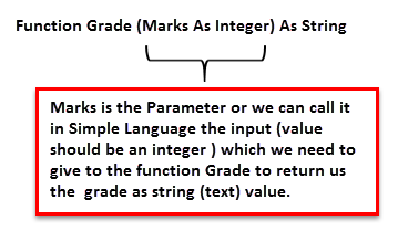
We can connect the object with its property or method using the period or dot (.) symbol.
How to Create Custom Functions using VBA?
You can download this VBA Function Excel Template here – VBA Function Excel Template
Example
Suppose we have the following data from a school where we need to find the total marks scored by the student, result, and grade.
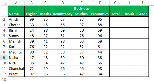
To sum up, the marks scored by an individual student in all subjects, we have an inbuilt function, SUM. But, determining the grade and result based on the criteria set out by the school is not available in Excel by default.
It is the reason why we need to create user-defined functions.
Step 1: Find Total Marks
First, we will find the total marks using the SUM function in excelThe SUM function in excel adds the numerical values in a range of cells. Being categorized under the Math and Trigonometry function, it is entered by typing “=SUM” followed by the values to be summed. The values supplied to the function can be numbers, cell references or ranges.read more.
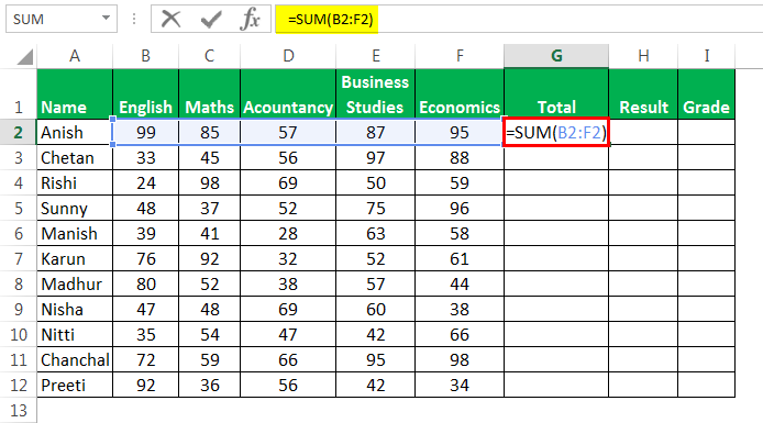
Then, press the “Enter” key to get the result.

Drag the formula to the rest of the cells.
Now, to find out the result (passed, failed, or essential repeat), the criteria set by the school is that.
- Suppose a student has scored more than or equal to 200 as total marks out of 500. In addition, suppose they have also not failed in any subject (scored more than 32 in each subject), a student is passed.
- If the student scored more than or equal to 200 but failed in 1 or 2 subjects, then a student will get “Essential Repeat” in those subjects.
- If the student has scored either less than 200 or fails in 3 or more subjects, then the student failed.
Step 2: Create ResultOfStudent Function
To create a function named ‘ResultOfStudent,’ we need to open “Visual Basic Editor” by using any of the methods below:
- Using the Developer tab excel.Enabling the developer tab in excel can help the user perform various functions for VBA, Macros and Add-ins like importing and exporting XML, designing forms, etc. This tab is disabled by default on excel; thus, the user needs to enable it first from the options menu.read more
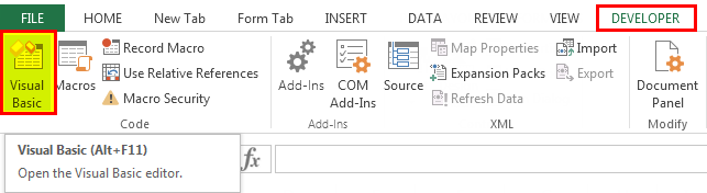
If the Developer tab is not available in MS Excel, then we can get that by using the following steps:
- Right-click anywhere on the ribbon. Then, choose to Customize the Ribbon in excelRibbons in Excel 2016 are designed to help you easily locate the command you want to use. Ribbons are organized into logical groups called Tabs, each of which has its own set of functions.read more‘.
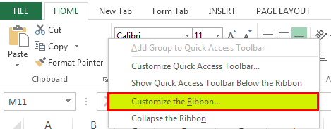
When we choose this command, the “Excel Options” dialog box opens.
- We need to check the box for “Developer” to get the tab.
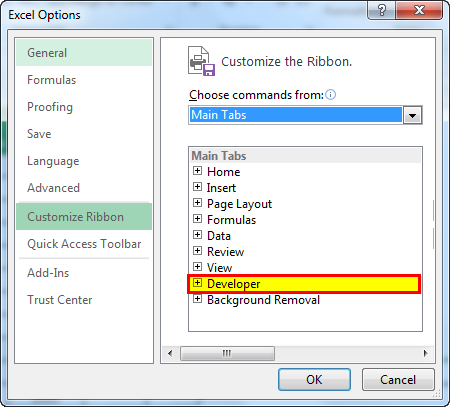
- Using the shortcut key, Alt+F11.

- When we open the VBA editorThe Visual Basic for Applications Editor is a scripting interface. These scripts are primarily responsible for the creation and execution of macros in Microsoft software.read more, we need to insert the module by going to the Insert menu and choosing a module.

- We need to paste the following code into the module.
Function ResultOfStudents(Marks As Range) As String

Dim mycell As Range
Dim Total As Integer
Dim CountOfFailedSubject As Integer

For Each mycell In Marks
Total = Total + mycell.Value

If mycell.Value < 33 Then
CountOfFailedSubject = CountOfFailedSubject + 1
End If

Next mycell
If Total >= 200 And CountOfFailedSubject <= 2 And CountOfFailedSubject > 0 Then
ResultOfStudents = "Essential Repeat"

ElseIf Total >= 200 And CountOfFailedSubject = 0 Then
ResultOfStudents = "Passed"

Else
ResultOfStudents = "Failed"
End If

End Function
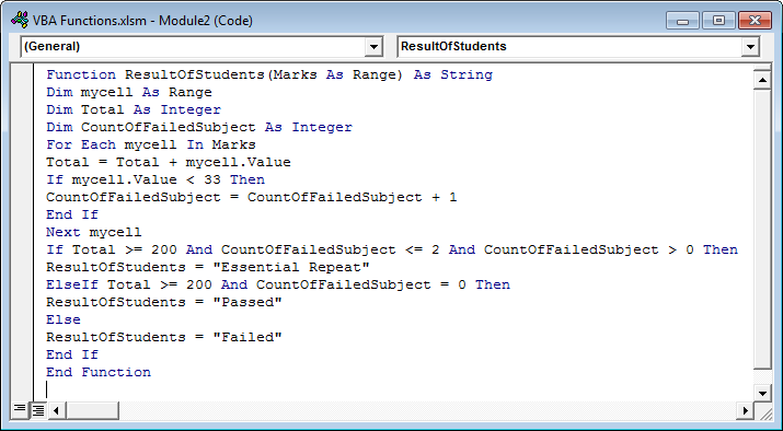
The above function returns the result for a student.
We need to understand how this code is working.
The first statement, ‘Function ResultOfStudents(Marks As Range) As String,’ declares a function named ‘ResultOfStudents’ that will accept a range as input for marks and return the result as a string.
Dim mycell As Range
Dim Total As Integer
Dim CountOfFailedSubject As Integer
These three statements declare variables, i.e.,
- ‘myCell’ as a Range,
- ‘Total’ as Integer (to store total marks scored by a student),
- ‘‘CountOfFailedSubject’ is an Integer (to store the number of subjects a student has failed).
For Each mycell In Marks
Total = Total + mycell.Value

If mycell.Value < 33 Then
CountOfFailedSubject = CountOfFailedSubject + 1
End If

Next mycell
This code checks for every cell in the ‘Marks’ range. It adds the value of every cell in the ‘Total’ variable. If the cell’s value is less than 33, add 1 to the ‘CountOfFailedSubject’ variable.
If Total >= 200 And CountOfFailedSubject <= 2 And CountOfFailedSubject > 0 Then
ResultOfStudents = "Essential Repeat"

ElseIf Total >= 200 And CountOfFailedSubject = 0 Then
ResultOfStudents = "Passed"

Else
ResultOfStudents = "Failed"
End If
This code checks the value of ‘Total’ and ‘CountOfFailedSubject’ and passes the ‘Essential Report,’ ‘Passed,’ or ‘Failed’ to the ‘ResultOfStudents.’
Step 3: Apply ResultOfStudents Function to Get Result
ResultOfStudents function takes marks, i.e., selecting 5 marks scored by the student.
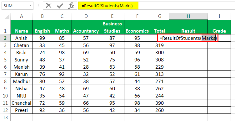
Now, select the range of cells, B2: F2.
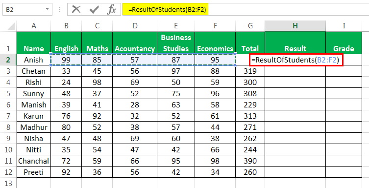
Drag the formula to the rest of the cells.
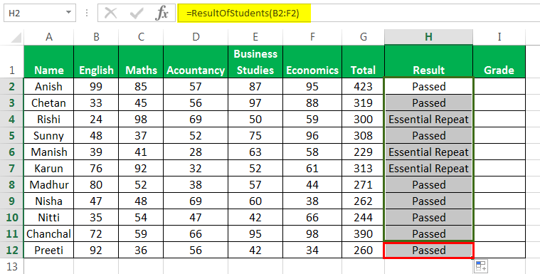
Step 4: Create ‘GradeForStudent’ Function to get Grades
Now to find out the grade for the student, we will create one more function named ‘GradeForStudent.’
The code would be:
Function GradeForStudent(TotalMarks As Integer, Result As String) As String

If TotalMarks > 440 And TotalMarks <= 500 And ((Result = "Passed" Or Result = "Essential Repeat")
Or Result = "Essential Repeat") Then GradeForStudent = "A"

ElseIf TotalMarks > 380 And TotalMarks <= 440 And (Result = "Passed" Or Result = "Essential Repeat") Then
GradeForStudent = "B"

ElseIf TotalMarks > 320 And TotalMarks <= 380 And (Result = "Passed" Or Result = "Essential Repeat") Then
GradeForStudent = "C"

ElseIf TotalMarks > 260 And TotalMarks <= 320 And (Result = "Passed" Or Result = "Essential Repeat") Then
GradeForStudent = "D"

ElseIf TotalMarks >= 200 And TotalMarks <= 260 And (Result = "Passed" Or Result = "Essential Repeat") Then
GradeForStudent = "E"

ElseIf TotalMarks < 200 Or Result = "Failed" Then
GradeForStudent = "F"

End If

End Function
This function assigns a ‘Grade’ to the student based on the ‘Total Marks’ and ‘Result.’
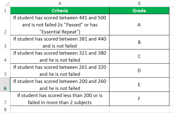
We need to write the formula and open the brackets in cell H2. Press Ctrl+Shift+A to find out the arguments.

The GradeForStudent function takes Total marks (sum of marks) and the result of the student as an argument to calculate the grade.
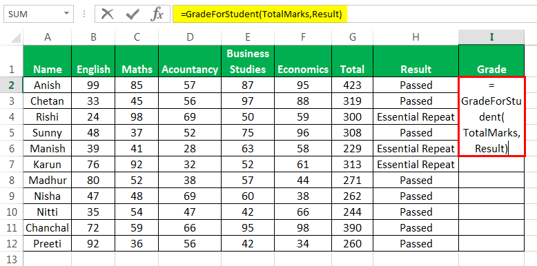
Now, select the individual cells, G2 and H2.
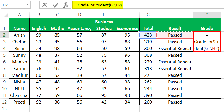
Now, we need to press Ctrl+D after selecting the cells to copy down the formulas.
We can highlight the values of less than 33 with the red background color to find out the subjects in which the student failed.

Recommended Articles
This article is a guide to VBA Functions. Here, we discuss creating custom functions using VBA code, practical examples, and a downloadable Excel template. You may learn more about VBA from the following articles:-
- VBA IIFThe «VBA IIF» condition evaluates the supplied expression or logical test and returns TRUE or FALSE as a result.read more
- SUMIF With VLOOKUPSUMIF is used to sum cells based on some condition, which takes arguments of range, criteria, or condition, and cells to sum. When there is a large amount of data available in multiple columns, we can use VLOOKUP as the criteria.read more
- Excel SUMIF Between Two DatesWhen we wish to work with data that has serial numbers with different dates and the condition to sum the values is based between two dates, we use Sumif between two dates. read more
- Excel VBA Delete RowIn VBA, to delete the command and to delete any rows together, the trick is that we give a single row reference if we need to delete a single row. However, for the multiple columns, we can provide numerous row references.read more