
Поиск повторяющихся значений (дубликатов) в одном из столбцов таблицы Excel и выделение их цветом заливки с помощью кода VBA.
Поиск дубликатов в столбце
Чаще всего повторяющиеся значения ищут в первом столбце таблицы, поэтому процедуру поиска дубликатов в VBA Excel рассмотрим именно на нем:
|
1 2 3 4 5 6 7 8 9 10 11 12 13 14 15 16 17 18 19 20 21 22 23 24 |
Sub DuplicateSearch() Dim ps As Long, myRange As Range, i1 As Long, i2 As Long ‘Определяем номер последней строки таблицы ps = Cells(1, 1).CurrentRegion.Rows.Count ‘Нет смысла искать дубликаты в таблице, состоящей из одной строки If ps > 1 Then ‘Присваиваем объектной переменной ссылку на исследуемый столбец Set myRange = Range(Cells(1, 1), Cells(ps, 1)) With myRange ‘Очищаем ячейки столбца от предыдущих закрашиваний .Interior.Color = xlNone For i1 = 1 To ps — 1 For i2 = i1 + 1 To ps If .Cells(i1) = .Cells(i2) Then ‘Если значения сравниваемых ячеек совпадают, ‘обеим присваиваем новый цвет заливки .Cells(i1).Interior.Color = 6740479 .Cells(i2).Interior.Color = 6740479 End If Next Next End With End If End Sub |
После ручного исправления или удаления повторяющихся значений, запускаем процедуру DuplicateSearch вновь, чтобы очистить от заливки ячейки столбца с уникальными значениями и заново выделить оставшиеся дубликаты.
Чтобы найти повторы в другом столбце, замените номер столбца в параметрах свойства Cells (в трех местах процедуры DuplicateSearch).
Константы для заливки
Для указания цвета заливки для ячеек с повторяющимися значениями вместо числового значения цвета можно использовать предопределенные константы:
| Предопределенная константа | Наименование цвета |
|---|---|
| vbBlack | Черный |
| vbBlue | Голубой |
| vbCyan | Бирюзовый |
| vbGreen | Зеленый |
| vbMagenta | Пурпурный |
| vbRed | Красный |
| vbWhite | Белый |
| vbYellow | Желтый |
| Цитата |
|---|
| Джек Восмеркин: Поиск дубликатов и пустых ячеек |
файла нет — поэтому ловите VBA (макрос) (для значений <= 255 символов)
xl дома пока отсутствует — тестирование за вами
| Код |
|---|
Sub ПоискПустыхИДублей () dim rng as range, cl as range, bad& set rng=selection bad=vbred for each cl in rng if len(cl)=0 or application.worksheetfunction.countif(rng,cl) <>1 then cl.interior.color=bad next cl |
аргументы функции могут быть другие, я имел ввиду — CountIf ([диапазон], [критерий]) — измените, в случае моей ошибки…
bad — код цвета, меняйте при необходимости, сейчас он «классический» красный и очень неудобный для зрительного восприятия.
Изменено: Jack Famous — 09.10.2018 17:25:58
|
0 / 0 / 0 Регистрация: 24.05.2008 Сообщений: 4 |
|
|
1 |
|
|
19.01.2009, 15:57. Показов 40057. Ответов 8
Регистрация: 19.01.2009 появилась необходимость поиска повторяющихся улиц с номерами домов в таблице эксель с помощью макроса Итак есть столбец «улица», рядом столбец «дом». Есть еще другие Столбцы в которых есть информация. Как можно было бы организовать алгоритм обхода так, чтобы это работало максимально производительно(быстро) во вложении к посту
0 |


|
32 / 32 / 4 Регистрация: 29.12.2008 Сообщений: 75 |
|
|
19.01.2009, 20:01 |
2 |
|
Пока не шочу слишком глубоко вдаваться в идею самого макроса, но думаю, гораздо удобнее сначала отсортировать таблицу excell по улицам в алфавитном порядке (макрос для этого можно не писать в ручную, а воспользоваться командой «Запись макроса» и выбрать сортировку по возрастанию или убыванию). В отсортированной таблице поиск повторяющихся элементов не должен занять много времени, особенно если воспользоваться «бинарным поиском». Примечание:
0 |
|
loter 2 / 2 / 0 Регистрация: 16.01.2009 Сообщений: 11 |
||||
|
20.01.2009, 22:43 |
3 |
|||
|
я в макросах не сильна, но эту задачу можно решить еще вот так:
по такому алгоритму у меня расчет занял 22 минуты 12 секунд. не знаю быстрее это или медленее чем у Вас, но мало ли… м.б. пригодится. если доступна сотировка, то есть более быстрый и простой механизм, только он делается не макросом, а формулой. сортируем сначала по а, затем по б и в пустой столбец во вторую строку забиваем формулу «=если((A2=A3)*И(B2=B3);1;»»)». растягиваем формулу до конца.
0 |
|
32 / 32 / 4 Регистрация: 29.12.2008 Сообщений: 75 |
|
|
21.01.2009, 18:19 |
4 |
|
Loter. Ты прав на все 100%. Однако вся прелесть макросов — это автоматизация твоих действий. Представь, что тебе каждый раз после ввода новых данных необходимо будет сначала отсортировать таблицу, потом выбрать специальный столбец, куда можно будет ввести предложенную тобой формулу с ЕСЛИ, растянуть ее (на несколько тысяч записей). Потом найти все строки, в которых твоя формула дает 1 и, наконец, выделив их, залить красным цветом. У-Ф-Ф-Ф… Даже рука устала писать. Гораздо проще все это проделать одним кликом по кнопке, который присвоен специальный макрос. Кстати.
0 |
|
loter 2 / 2 / 0 Регистрация: 16.01.2009 Сообщений: 11 |
||||
|
22.01.2009, 18:01 |
5 |
|||
|
хм….
на базу в 6000 заняло меньше 5 секунд
0 |
|
maximus09 32 / 32 / 4 Регистрация: 29.12.2008 Сообщений: 75 |
||||
|
23.01.2009, 17:57 |
6 |
|||
|
Не знаю как bloogrox, а я результатом в общем и целом удовлетворен. Единственное, на что нужно обратить внимание — это то, что сейчас программа использует дополнительный столбец книги Excell для того чтобы ввести формулу
Это не всегда хорошо. Поиск можно осуществить простым перебором ячеек, не выводя никакой дополнительной информации на листы книги Excell.
0 |
|
2 / 2 / 0 Регистрация: 16.01.2009 Сообщений: 11 |
|
|
23.01.2009, 20:16 |
7 |
|
maximus09, а о каких встроенных механизмах сортировки ты говорил?
0 |
|
32 / 32 / 4 Регистрация: 29.12.2008 Сообщений: 75 |
|
|
23.01.2009, 20:39 |
8 |
|
Почитай мое первое сообщение. Там найдешь такие слова: (макрос для этого можно не писать в ручную, а воспользоваться командой «Запись макроса» и выбрать сортировку по возрастанию или убыванию). В отсортированной таблице поиск повторяющихся элементов не должен занять много времени, особенно если воспользоваться «бинарным поиском». Примечание: Если перед выбором команды Данные -> Сортировка выбрать команду Сервис ->Макрос->Начать запись, а после того, как сортировка выполнится вручную остановить запись макроса, то Excell автоматически сама создаст макрос сортировки. Программисту останется только его немножко подправить под свои нужды и включить то, что получится в итоге, в текст программы поиска повторяющихся элементов. Более подробно об описанном здесь механизме программирования можно прочитать в книге Кстати, там данный пример ручной с сортировкой описан в подробностях (что, какие опции в окне параметров сортировки нужно выбирать, зачем нужно выделять всю таблицу прежде чем производить сортировку и т.п.). Очень рекомендую книгу. Сам учился по ней. Но, стоит сказать, что она целиком посвящена VBA в Excell.
0 |
|
2 / 2 / 0 Регистрация: 16.01.2009 Сообщений: 11 |
|
|
24.01.2009, 07:03 |
9 |
|
спасибо. книжку посмотрю.
0 |
|
IT_Exp Эксперт 87844 / 49110 / 22898 Регистрация: 17.06.2006 Сообщений: 92,604 |
24.01.2009, 07:03 |
|
9 |
Want to find duplicates in a column in excel and want to popup a msgbox upon finding even 1 duplicate and it shouldn’t keep on popping messages if it finds more than one duplicate.
Also, if i can use two column cell values and use that together to find duplicates, this would be also helpful.
  Sub ColumnDuplicates()
    Dim lastRow As Long
    Dim matchFoundIndex As Long
    Dim iCntr As Long
    lastRow = Range("A65000").End(xlUp).Row

    For iCntr = 1 To lastRow
    If Cells(iCntr, 1) <> "" Then
        matchFoundIndex = WorksheetFunction.Match(Cells(iCntr, 1), Range("A1:A" & lastRow), 0)
        If iCntr <> matchFoundIndex Then
            MsgBox ("There are duplicates in Column A")
        End If
    End If
    Next
    MsgBox ("No Duplicates in Column A")
End Sub
Expecting to print message saying that column A has duplicates or does not have duplicates
![]()
asked Jul 26, 2019 at 15:15
![]()
7
What about the use of EVALUATE?
Public Sub Test()

With ThisWorkbook.Sheets("Sheet1")
    lr = .Cells(.Rows.Count, "A").End(xlUp).Row
    If .Evaluate("=Max(countif(A1:A" & lr & ",A1:A" & lr & "))") > 1 Then
        MsgBox "Duplicates!"
    Else
        MsgBox "No Duplicates!"
    End If
End With

End Sub
Or, parameterized:
Public Sub Test(ByVal sheet As Worksheet, ByVal columnHeading As String)

With sheet
    lr = .Cells(.Rows.Count, columnHeading).End(xlUp).Row
    If .Evaluate("=Max(countif(" & columnHeading & "1:" & columnHeading & lr & "," & columnHeading & "1:" & columnHeading & lr & "))") > 1 Then
        MsgBox "Duplicates!"
    Else
        MsgBox "No Duplicates!"
    End If
End With

End Sub
Now you can invoke it like this:
Test Sheet1, "A" ' find dupes in ThisWorkbook/Sheet1 in column A
Test Sheet2, "B" ' find dupes in ThisWorkbook/Sheet2 in column B
Test ActiveWorkbook.Worksheets("SomeSheet"), "Z" ' find dupes in "SomeSheet" worksheet of whatever workbook is currently active, in column Z
![]()
answered Jul 26, 2019 at 15:37
![]()
JvdVJvdV
66.6k8 gold badges38 silver badges68 bronze badges
19
Throw your values in a dictionary
Sub ColumnDuplicates()
Dim lastRow As Long
Dim matchFoundIndex As Long
Dim iCntr As Long

lastRow = Range("A65000").End(xlUp).Row
Set oDictionary = CreateObject("Scripting.Dictionary")
For iCntr = 1 To lastRow
    If Cells(iCntr, 1) <> "" Then
        If oDictionary.Exists(Cells(iCntr, 1).Value) Then
            MsgBox ("There are duplicates in Column A")
            Exit Sub
        Else
            oDictionary.Add Cells(iCntr, 1).Value, Cells(iCntr, 1).Value
        End If
    End If
Next
MsgBox ("No Duplicates in Column A")
End Sub
![]()
answered Jul 26, 2019 at 15:23
![]()
TimTim
2,6333 gold badges25 silver badges47 bronze badges
5
If you have Excel 2007+ then this will be faster. This code ran in 1 sec for 200k rows
Sub Sample()
    Debug.Print Now

    Dim ws As Worksheet
    Dim wsTemp As Worksheet

    Set ws = Sheet1

    Set wsTemp = ThisWorkbook.Sheets.Add

    ws.Columns(1).Copy wsTemp.Columns(1)

    wsTemp.Columns(1).RemoveDuplicates Columns:=1, Header:=xlNo

    If Application.WorksheetFunction.CountA(ws.Columns(1)) <> _
       Application.WorksheetFunction.CountA(wsTemp.Columns(1)) Then
        Debug.Print "There are duplicates in Col A"
    Else
        Debug.Print "duplicates found in Col A"
    End If

    Application.DisplayAlerts = False
    wsTemp.Delete
    Application.DisplayAlerts = True

    Debug.Print Now
End Sub
I used the below code to generate 200k records in Col A
Sub GenerateSampleData()
    Range("A1:A200000").Formula = "=Row()"
    Range("A1:A200000").Value = Range("A1:A200000").Value
    Range("A10000:A20000").Value = Range("A20000:A30000").Value
End Sub
Code execution

answered Jul 26, 2019 at 15:51
![]()
Siddharth RoutSiddharth Rout
146k17 gold badges206 silver badges250 bronze badges
Excel для Microsoft 365 Excel для Microsoft 365 для Mac Excel 2021 Excel 2021 для Mac Excel 2019 Excel 2019 для Mac Excel 2016 Excel 2016 для Mac Excel 2013 Office для бизнеса Excel 2010 Excel 2007 Еще…Меньше
Чтобы сравнить данные в двух столбцах Microsoft Excel и найти повторяющиеся записи, воспользуйтесь следующими способами.
Способ 1. Использование формулы на этом этапе
-
Начните Excel.
-
На новом примере введите следующие данные (оставьте столбец B пустым):
A
B
C
1
1
3
2
2
5
3
3
8
4
4
2
5
5
0
-
Введите в ячейку B1 следующую
формулу:=IF(ISERROR(MATCH(A1,$C$1:$C$5,0)),»»,A1)
-
Выберем ячейку С1 по B5.
-
В Excel 2007 и более поздних версиях Excel выберите Заполнить в группе Редактирование, а затем выберите Вниз.
Повторяющиеся числа отображаются в столбце B, как в следующем примере:
A
B
C
1
1
3
2
2
2
5
3
3
3
8
4
4
2
5
5
5
0
Способ 2. Использование макроса Visual Basic макроса
Предупреждение: Корпорация Майкрософт предоставляет примеры программирования только для иллюстрации без гарантии, выраженной или подразумеваемой. Это относится и не только к подразумеваемой гарантии пригодности и пригодности для определенной цели. В этой статье предполагается, что вы знакомы с языком программирования, который демонстрируется, и средствами, используемыми для создания и от debug procedures. Инженеры службы поддержки Майкрософт могут объяснить функциональные возможности конкретной процедуры. Однако они не будут изменять эти примеры, чтобы обеспечить дополнительные функциональные возможности или процедуры по построению в необходимом порядке.
Чтобы использовать макрос Visual Basic для сравнения данных в двух столбцах, с помощью следующих действий:
-
Запустите Excel.
-
Нажмите ALT+F11, чтобы запустить Visual Basic редактора.
-
В меню Вставка выберите Модуль.
-
Введите следующий код на листе модуля:
Sub Find_Matches() Dim CompareRange As Variant, x As Variant, y As Variant ' Set CompareRange equal to the range to which you will ' compare the selection. Set CompareRange = Range("C1:C5") ' NOTE: If the compare range is located on another workbook ' or worksheet, use the following syntax. ' Set CompareRange = Workbooks("Book2"). _ ' Worksheets("Sheet2").Range("C1:C5") ' ' Loop through each cell in the selection and compare it to ' each cell in CompareRange. For Each x In Selection For Each y In CompareRange If x = y Then x.Offset(0, 1) = x Next y Next x End Sub -
Нажмите ALT+F11, чтобы вернуться к Excel.
-
Введите в качестве примера следующие данные (оставьте столбец B пустым):
A
B
C
1
1
3
2
2
5
3
3
8
4
4
2
5
5
0
-
-
Выберем ячейку от A1 до A5.
-
В Excel 2007 и более поздних версиях Excel выберите вкладку Разработчик, а затем в группе Код выберите макрос.
Примечание: Если вкладка Разработчик не отключается, возможно, ее нужно включить. Для этого выберите Файл > параметры > настроитьленту , а затем выберите вкладку Разработчик в поле настройки справа.
-
Щелкните Find_Matches, а затем нажмите кнопку Выполнить.
Повторяющиеся числа отображаются в столбце B. Совпадающие числа будут поместиться рядом с первым столбцом, как показано ниже.
A
B
C
1
1
3
2
2
2
5
3
3
3
8
4
4
2
5
5
5
0
Нужна дополнительная помощь?
You can achieve the desired effect by using «Conditional Formatting» feature in Excel Worksheet:
-
Select Column A
-
Click on Conditional Formatting menu button, then select «Highlight Cells Rules» and «Duplicates Values»: specify the color from Drop-Down list.
-
Repeat the same steps for other Columns.
In case you prefer to use your VBA solution which highlights duplicates with different colors, then just apply it to other Columns: see that line
Set rng = Range("A1:A" & Range("A1048576").End(xlUp).Row)
so, instead of Column «A» use Column «B», etc. I would recommend to use iteration through the specified Columns range. With minor changes it can be implemented as shown in the following sample code snippet:
Sub DupEntry()
Dim cel As Variant
Dim rng As Range
Dim clr As Long
Application.ScreenUpdating = False
Application.Calculation = xlCalculationManual

'Sample Array of Columns
Dim Col(1 To 3) As String
Col(1) = "A"
Col(2) = "B"
Col(3) = "C"

'Iterate through Columns
For i = 1 To 3
    'Set rng = Range("A1:A" & Range("A1048576").End(xlUp).Row)
    Set rng = Range(Col(i) & "1:" & Col(i) & Range(Col(i) & "1048576").End(xlUp).Row)
    rng.Interior.ColorIndex = xlNone
    clr = 3
    For Each cel In rng
        If Application.WorksheetFunction.CountIf(rng, cel) > 1 Then
            'If Application.WorksheetFunction.CountIf(Range("A1:A" & cel.Row), cel) = 1 Then
            If Application.WorksheetFunction.CountIf(Range(Col(i) & "1:" & Col(i) & cel.Row), cel) = 1 Then
                cel.Interior.ColorIndex = clr
                clr = clr + 1
            Else
                cel.Interior.ColorIndex = rng.Cells(WorksheetFunction.Match(cel.Value, rng, False), 1).Interior.ColorIndex
            End If
        End If
    Next
Next i
Application.ScreenUpdating = True
Application.Calculation = xlCalculationAutomatic
End Sub
(original code lines are commented off). Alternatively, you can use cells R1C1 notation.
Hope this will help. Best regards,
In this Article
- RemoveDuplicates Method
- RemoveDuplicates Usage Notes
- Sample Data for VBA Examples
- Remove Duplicate Rows
- Remove Duplicates Comparing Multiple Columns
- Removing Duplicate Rows from a Table
- Remove Duplicates From Arrays
- Removing Duplicates from Rows of Data Using VBA
This tutorial will demonstrate how to remove duplicates using the RemoveDuplicates method in VBA.
RemoveDuplicates Method
When data is imported or pasted into an Excel worksheet, it can often contain duplicate values. You may need to clean the incoming data and remove duplicates.
Fortunately, there is an easy method within the Range object of VBA which allows you to do this.
Range(“A1:C8”).RemoveDuplicates Columns:=1, Header:=xlYesSyntax is:
RemoveDuplicates([Columns],[Header]
- [Columns] – Specify which columns are checked for duplicate values. All columns much match to be considered a duplicate.
- [Header] – Does data have a header? xlNo (default), xlYes, xlYesNoGuess
Technically, both parameters are optional. However, if you don’t specify the Columns argument, no duplicates will be removed.
The default value for Header is xlNo. Of course it’s better to specify this argument, but if you have a header row, it’s unlikely the header row will match as a duplicate.
RemoveDuplicates Usage Notes
- Before using the RemoveDuplicates method, you must specify a range to be used.
- The RemoveDuplicates method will remove any rows with duplicates found, but will keep the original row with all values.
- The RemoveDuplicates method only works on columns and not on rows, but VBA code can be written to rectify this situation (see later).
Sample Data for VBA Examples
In order to show how the example code works, the following sample data is used:
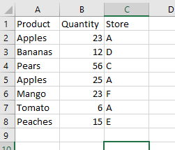
Remove Duplicate Rows
This code will remove all duplicate rows based only on values in column A:
Sub RemoveDupsEx1()
Range(“A1:C8”).RemoveDuplicates Columns:=1, Header:=xlYes
End Sub
Notice that we explicitly defined the Range “A1:C8”. Instead you can used the UsedRange. The UsedRange will determine the last used row and column of your data and apply RemoveDuplicates to that entire range:
Sub RemoveDups_UsedRange()
ActiveSheet.UsedRange.RemoveDuplicates Columns:=1, Header:=xlYes
End Sub
UsedRange is incredibly useful, removing the need for you to explicitly define the range.
After running these code, your worksheet will now look like this:
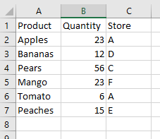
Notice that because only column A (column 1) was specified, the ‘Apples’ duplicate formerly in row 5 has been removed. However, the Quantity (column 2) is different.
To remove duplicates, comparing multiple columns, we can specify those columns using an Array method.
Remove Duplicates Comparing Multiple Columns
Sub RemoveDups_MultColumns()
ActiveSheet.UsedRange.RemoveDuplicates Columns:=Array(1, 2) , Header:=xlYes
End Sub
The Array tells VBA to compare the data using both columns 1 and 2 (A and B).
The columns in the array do not have to be in consecutive order.
Sub SimpleExample()
ActiveSheet.UsedRange.RemoveDuplicates Columns:=Array(3, 1) , Header:=xlYes
End Sub
In this example, columns 1 and 3 are used for the duplicate comparison.
This code example uses all three columns to check for duplicates:
Sub SimpleExample()
ActiveSheet.UsedRange.RemoveDuplicates Columns:=Array(1, 2, 3) , Header:=xlYes
End Sub
Removing Duplicate Rows from a Table
The RemoveDuplicates can also be applied to an Excel table in exactly the same way. However, the syntax is slightly different.
Sub SimpleExample()
ActiveSheet.ListObjects("Table1").DataBodyRange.RemoveDuplicates Columns:=Array(1, 3), _
Header:=xlYes
End Sub
This will remove the duplicates in the table based on columns 1 and 3 (A and C). However, it does not tidy up the color formatting of the table, and you will see colored blank rows left behind at the bottom of the table.
VBA Coding Made Easy
Stop searching for VBA code online. Learn more about AutoMacro — A VBA Code Builder that allows beginners to code procedures from scratch with minimal coding knowledge and with many time-saving features for all users!

Learn More
Remove Duplicates From Arrays
If you need to remove duplicate values from an array, of course you can output your array into Excel, use the RemoveDuplicates method, and re-import the array.
However, we also wrote a VBA procedure to remove duplicates from an array.
Removing Duplicates from Rows of Data Using VBA
The RemoveDuplicates method only works on columns of data, but with some ‘out of the box’ thinking, you can create a VBA procedure to deal with rows of data.
Suppose that your data looks like this on your worksheet:
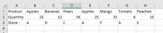
You have the same duplicates as before in columns B and E, but you cannot remove them using the RemoveDuplicates method.
The answer is to use VBA to create an additional worksheet, copy the data into it transposing it into columns, remove the duplicates, and then copy it back transposing it back into rows.
Sub DuplicatesInRows()
    'Turn off screen updating and alerts – we want the code to run smoothly without the user seeing
    ‘what is going on
    Application.ScreenUpdating = False
    Application.DisplayAlerts = False
    'Add a new worksheet
    Sheets.Add After:=ActiveSheet
    'Call the new worksheet 'CopySheet'
    ActiveSheet.Name = "CopySheet"
    'Copy the data from the original worksheet
    Sheets("DataInRows").UsedRange.Copy
    'Activate the new sheet that has been created
    Sheets("CopySheet").Activate
    'Paste transpose the data so that it is now in columns
    ActiveSheet.Range("A1").PasteSpecial Paste:=xlPasteAll, Operation:=xlNone, SkipBlanks:= _
        False, Transpose:=True
   'Remove the duplicates for columns 1 and 3
    ActiveSheet.UsedRange.RemoveDuplicates Columns:=Array(1, 3), Header _
        :=xlYes
    'Clear the data in the original worksheet
    Sheets("DataInRows").UsedRange.ClearContents
    'Copy the columns of data from the new worksheet created
   Sheets("Copysheet").UsedRange.Copy
   'Activate the original sheet
    Sheets("DataInRows").Activate

   'Paste transpose the non-duplicate data
    ActiveSheet.Range("A1").PasteSpecial Paste:=xlPasteAll, Operation:=xlNone, SkipBlanks:= _
        False, Transpose:=True
    'Delete the copy sheet - no longer needed
    Sheets("Copysheet").Delete
    'Activate the original sheet
    Sheets("DataInRows").Activate
    'Turn back on screen updating and alerts
    Application.ScreenUpdating = True
    Application.DisplayAlerts = True
End Sub
This code assumes that the original data in rows is held on a worksheet called ‘DataInRows’
After running the code, your worksheet will look like this:
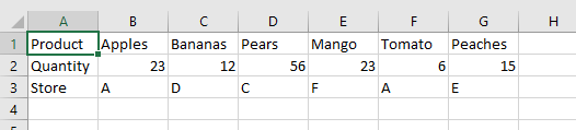
The ‘Apples’ duplicate in column E has now been removed. The user is back in a clean position, with no extraneous worksheets hanging around, and the whole process has been done smoothly with no screen flickering or warning messages.