
Вырезание, перемещение, копирование и вставка ячеек (диапазонов) в VBA Excel. Методы Cut, Copy и PasteSpecial объекта Range, метод Paste объекта Worksheet.
Метод Range.Cut
Range.Cut – это метод, который вырезает объект Range (диапазон ячеек) в буфер обмена или перемещает его в указанное место на рабочем листе.
Синтаксис
Параметры
| Параметры | Описание |
|---|---|
| Destination | Необязательный параметр. Диапазон ячеек рабочего листа, в который будет вставлен (перемещен) вырезанный объект Range (достаточно указать верхнюю левую ячейку диапазона). Если этот параметр опущен, объект вырезается в буфер обмена. |
Для вставки на рабочий лист диапазона ячеек, вырезанного в буфер обмена методом Range.Cut, следует использовать метод Worksheet.Paste.
Метод Range.Copy
Range.Copy – это метод, который копирует объект Range (диапазон ячеек) в буфер обмена или в указанное место на рабочем листе.
Синтаксис
Параметры
| Параметры | Описание |
|---|---|
| Destination | Необязательный параметр. Диапазон ячеек рабочего листа, в который будет вставлен скопированный объект Range (достаточно указать верхнюю левую ячейку диапазона). Если этот параметр опущен, объект копируется в буфер обмена. |
Метод Worksheet.Paste
Worksheet.Paste – это метод, который вставляет содержимое буфера обмена на рабочий лист.
Синтаксис
|
Worksheet.Paste (Destination, Link) |
Метод Worksheet.Paste работает как с диапазонами ячеек, вырезанными в буфер обмена методом Range.Cut, так и скопированными в буфер обмена методом Range.Copy.
Параметры
| Параметры | Описание |
|---|---|
| Destination | Необязательный параметр. Диапазон (ячейка), указывающий место вставки содержимого буфера обмена. Если этот параметр не указан, используется текущий выделенный объект. |
| Link | Необязательный параметр. Булево значение, которое указывает, устанавливать ли ссылку на источник вставленных данных: True – устанавливать, False – не устанавливать (значение по умолчанию). |
В выражении с методом Worksheet.Paste можно указать только один из параметров: или Destination, или Link.
Для вставки из буфера обмена отдельных компонентов скопированных ячеек (значения, форматы, примечания и т.д.), а также для проведения транспонирования и вычислений, используйте метод Range.PasteSpecial (специальная вставка).
Примеры
Вырезание и вставка диапазона одной строкой (перемещение):
|
Range(«A1:C3»).Cut Range(«E1») |
Вырезание ячеек в буфер обмена и вставка методом ActiveSheet.Paste:
|
Range(«A1:C3»).Cut ActiveSheet.Paste Range(«E1») |
Копирование и вставка диапазона одной строкой:
|
Range(«A18:C20»).Copy Range(«E18») |
Копирование ячеек в буфер обмена и вставка методом ActiveSheet.Paste:
|
Range(«A18:C20»).Copy ActiveSheet.Paste Range(«E18») |
Копирование одной ячейки и вставка ее данных во все ячейки заданного диапазона:
|
Range(«A1»).Copy Range(«B1:D10») |
When working with Excel, most of your time is spent in the worksheet area – dealing with cells and ranges.
And if you want to automate your work in Excel using VBA, you need to know how to work with cells and ranges using VBA.
There are a lot of different things you can do with ranges in VBA (such as select, copy, move, edit, etc.).
So to cover this topic, I will break this tutorial into sections and show you how to work with cells and ranges in Excel VBA using examples.
Let’s get started.
All the codes I mention in this tutorial need to be placed in the VB Editor. Go to the ‘Where to Put the VBA Code‘ section to know how it works.
If you’re interested in learning VBA the easy way, check out my Online Excel VBA Training.
Selecting a Cell / Range in Excel using VBA
To work with cells and ranges in Excel using VBA, you don’t need to select it.
In most of the cases, you are better off not selecting cells or ranges (as we will see).
Despite that, it’s important you go through this section and understand how it works. This will be crucial in your VBA learning and a lot of concepts covered here will be used throughout this tutorial.
So let’s start with a very simple example.
Selecting a Single Cell Using VBA
If you want to select a single cell in the active sheet (say A1), then you can use the below code:
Sub SelectCell()
Range("A1").Select
End Sub
The above code has the mandatory ‘Sub’ and ‘End Sub’ part, and a line of code that selects cell A1.
Range(“A1”) tells VBA the address of the cell that we want to refer to.
Select is a method of the Range object and selects the cells/range specified in the Range object. The cell references need to be enclosed in double quotes.
This code would show an error in case a chart sheet is an active sheet. A chart sheet contains charts and is not widely used. Since it doesn’t have cells/ranges in it, the above code can’t select it and would end up showing an error.
Note that since you want to select the cell in the active sheet, you just need to specify the cell address.
But if you want to select the cell in another sheet (let’s say Sheet2), you need to first activate Sheet2 and then select the cell in it.
Sub SelectCell()
Worksheets("Sheet2").Activate
Range("A1").Select
End Sub
Similarly, you can also activate a workbook, then activate a specific worksheet in it, and then select a cell.
Sub SelectCell()
Workbooks("Book2.xlsx").Worksheets("Sheet2").Activate
Range("A1").Select
End Sub
Note that when you refer to workbooks, you need to use the full name along with the file extension (.xlsx in the above code). In case the workbook has never been saved, you don’t need to use the file extension.
Now, these examples are not very useful, but you will see later in this tutorial how we can use the same concepts to copy and paste cells in Excel (using VBA).
Just as we select a cell, we can also select a range.
In case of a range, it could be a fixed size range or a variable size range.
In a fixed size range, you would know how big the range is and you can use the exact size in your VBA code. But with a variable-sized range, you have no idea how big the range is and you need to use a little bit of VBA magic.
Let’s see how to do this.
Selecting a Fix Sized Range
Here is the code that will select the range A1:D20.
Sub SelectRange()
Range("A1:D20").Select
End Sub
Another way of doing this is using the below code:
Sub SelectRange()
Range("A1", "D20").Select
End Sub
The above code takes the top-left cell address (A1) and the bottom-right cell address (D20) and selects the entire range. This technique becomes useful when you’re working with variably sized ranges (as we will see when the End property is covered later in this tutorial).
If you want the selection to happen in a different workbook or a different worksheet, then you need to tell VBA the exact names of these objects.
For example, the below code would select the range A1:D20 in Sheet2 worksheet in the Book2 workbook.
Sub SelectRange()
Workbooks("Book2.xlsx").Worksheets("Sheet1").Activate
Range("A1:D20").Select
End Sub
Now, what if you don’t know how many rows are there. What if you want to select all the cells that have a value in it.
In these cases, you need to use the methods shown in the next section (on selecting variably sized range).
Selecting a Variably Sized Range
There are different ways you can select a range of cells. The method you choose would depend on how the data is structured.
In this section, I will cover some useful techniques that are really useful when you work with ranges in VBA.
Select Using CurrentRange Property
In cases where you don’t know how many rows/columns have the data, you can use the CurrentRange property of the Range object.
The CurrentRange property covers all the contiguous filled cells in a data range.
Below is the code that will select the current region that holds cell A1.
Sub SelectCurrentRegion()
Range("A1").CurrentRegion.Select
End Sub
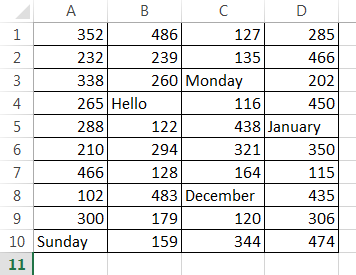
The above method is good when you have all data as a table without any blank rows/columns in it.
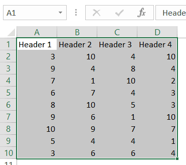
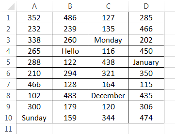
But in case you have blank rows/columns in your data, it will not select the ones after the blank rows/columns. In the image below, the CurrentRegion code selects data till row 10 as row 11 is blank.
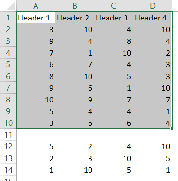
In such cases, you may want to use the UsedRange property of the Worksheet Object.
Select Using UsedRange Property
UsedRange allows you to refer to any cells that have been changed.
So the below code would select all the used cells in the active sheet.
Sub SelectUsedRegion()
ActiveSheet.UsedRange.Select
End Sub
Note that in case you have a far-off cell that has been used, it would be considered by the above code and all the cells till that used cell would be selected.
Select Using the End Property
Now, this part is really useful.
The End property allows you to select the last filled cell. This allows you to mimic the effect of Control Down/Up arrow key or Control Right/Left keys.
Let’s try and understand this using an example.
Suppose you have a dataset as shown below and you want to quickly select the last filled cells in column A.
The problem here is that data can change and you don’t know how many cells are filled. If you have to do this using keyboard, you can select cell A1, and then use Control + Down arrow key, and it will select the last filled cell in the column.
Now let’s see how to do this using VBA. This technique comes in handy when you want to quickly jump to the last filled cell in a variably-sized column
Sub GoToLastFilledCell()
Range("A1").End(xlDown).Select
End Sub
The above code would jump to the last filled cell in column A.
Similarly, you can use the End(xlToRight) to jump to the last filled cell in a row.
Sub GoToLastFilledCell()
Range("A1").End(xlToRight).Select
End Sub
Now, what if you want to select the entire column instead of jumping to the last filled cell.
You can do that using the code below:
Sub SelectFilledCells()
Range("A1", Range("A1").End(xlDown)).Select
End Sub
In the above code, we have used the first and the last reference of the cell that we need to select. No matter how many filled cells are there, the above code will select all.
Remember the example above where we selected the range A1:D20 by using the following line of code:
Range(“A1″,”D20”)
Here A1 was the top-left cell and D20 was the bottom-right cell in the range. We can use the same logic in selecting variably sized ranges. But since we don’t know the exact address of the bottom-right cell, we used the End property to get it.
In Range(“A1”, Range(“A1”).End(xlDown)), “A1” refers to the first cell and Range(“A1”).End(xlDown) refers to the last cell. Since we have provided both the references, the Select method selects all the cells between these two references.
Similarly, you can also select an entire data set that has multiple rows and columns.
The below code would select all the filled rows/columns starting from cell A1.
Sub SelectFilledCells()
Range("A1", Range("A1").End(xlDown).End(xlToRight)).Select
End Sub
In the above code, we have used Range(“A1”).End(xlDown).End(xlToRight) to get the reference of the bottom-right filled cell of the dataset.
Difference between Using CurrentRegion and End
If you’re wondering why use the End property to select the filled range when we have the CurrentRegion property, let me tell you the difference.
With End property, you can specify the start cell. For example, if you have your data in A1:D20, but the first row are headers, you can use the End property to select the data without the headers (using the code below).
Sub SelectFilledCells()
Range("A2", Range("A2").End(xlDown).End(xlToRight)).Select
End Sub
But the CurrentRegion would automatically select the entire dataset, including the headers.
So far in this tutorial, we have seen how to refer to a range of cells using different ways.
Now let’s see some ways where we can actually use these techniques to get some work done.
Copy Cells / Ranges Using VBA
As I mentioned at the beginning of this tutorial, selecting a cell is not necessary to perform actions on it. You will see in this section how to copy cells and ranges without even selecting these.
Let’s start with a simple example.
Copying Single Cell
If you want to copy cell A1 and paste it into cell D1, the below code would do it.
Sub CopyCell()
Range("A1").Copy Range("D1")
End Sub
Note that the copy method of the range object copies the cell (just like Control +C) and pastes it in the specified destination.
In the above example code, the destination is specified in the same line where you use the Copy method. If you want to make your code even more readable, you can use the below code:
Sub CopyCell()
Range("A1").Copy Destination:=Range("D1")
End Sub
The above codes will copy and paste the value as well as formatting/formulas in it.
As you might have already noticed, the above code copies the cell without selecting it. No matter where you’re on the worksheet, the code will copy cell A1 and paste it on D1.
Also, note that the above code would overwrite any existing code in cell D2. If you want Excel to let you know if there is already something in cell D1 without overwriting it, you can use the code below.
Sub CopyCell()
If Range("D1") <> "" Then
Response = MsgBox("Do you want to overwrite the existing data", vbYesNo)
End If
If Response = vbYes Then
Range("A1").Copy Range("D1")
End If
End Sub
Copying a Fix Sized Range
If you want to copy A1:D20 in J1:M20, you can use the below code:
Sub CopyRange()
Range("A1:D20").Copy Range("J1")
End Sub
In the destination cell, you just need to specify the address of the top-left cell. The code would automatically copy the exact copied range into the destination.
You can use the same construct to copy data from one sheet to the other.
The below code would copy A1:D20 from the active sheet to Sheet2.
Sub CopyRange()
Range("A1:D20").Copy Worksheets("Sheet2").Range("A1")
End Sub
The above copies the data from the active sheet. So make sure the sheet that has the data is the active sheet before running the code. To be safe, you can also specify the worksheet’s name while copying the data.
Sub CopyRange()
Worksheets("Sheet1").Range("A1:D20").Copy Worksheets("Sheet2").Range("A1")
End Sub
The good thing about the above code is that no matter which sheet is active, it will always copy the data from Sheet1 and paste it in Sheet2.
You can also copy a named range by using its name instead of the reference.
For example, if you have a named range called ‘SalesData’, you can use the below code to copy this data to Sheet2.
Sub CopyRange()
Range("SalesData").Copy Worksheets("Sheet2").Range("A1")
End Sub
If the scope of the named range is the entire workbook, you don’t need to be on the sheet that has the named range to run this code. Since the named range is scoped for the workbook, you can access it from any sheet using this code.
If you have a table with the name Table1, you can use the below code to copy it to Sheet2.
Sub CopyTable()
Range("Table1[#All]").Copy Worksheets("Sheet2").Range("A1")
End Sub
You can also copy a range to another Workbook.
In the following example, I copy the Excel table (Table1), into the Book2 workbook.
Sub CopyCurrentRegion()
Range("Table1[#All]").Copy Workbooks("Book2.xlsx").Worksheets("Sheet1").Range("A1")
End Sub
This code would work only if the Workbook is already open.
Copying a Variable Sized Range
One way to copy variable sized ranges is to convert these into named ranges or Excel Table and the use the codes as shown in the previous section.
But if you can’t do that, you can use the CurrentRegion or the End property of the range object.
The below code would copy the current region in the active sheet and paste it in Sheet2.
Sub CopyCurrentRegion()
Range("A1").CurrentRegion.Copy Worksheets("Sheet2").Range("A1")
End Sub
If you want to copy the first column of your data set till the last filled cell and paste it in Sheet2, you can use the below code:
Sub CopyCurrentRegion()
Range("A1", Range("A1").End(xlDown)).Copy Worksheets("Sheet2").Range("A1")
End Sub
If you want to copy the rows as well as columns, you can use the below code:
Sub CopyCurrentRegion()
Range("A1", Range("A1").End(xlDown).End(xlToRight)).Copy Worksheets("Sheet2").Range("A1")
End Sub
Note that all these codes don’t select the cells while getting executed. In general, you will find only a handful of cases where you actually need to select a cell/range before working on it.
Assigning Ranges to Object Variables
So far, we have been using the full address of the cells (such as Workbooks(“Book2.xlsx”).Worksheets(“Sheet1”).Range(“A1”)).
To make your code more manageable, you can assign these ranges to object variables and then use those variables.
For example, in the below code, I have assigned the source and destination range to object variables and then used these variables to copy data from one range to the other.
Sub CopyRange()
Dim SourceRange As Range
Dim DestinationRange As Range
Set SourceRange = Worksheets("Sheet1").Range("A1:D20")
Set DestinationRange = Worksheets("Sheet2").Range("A1")
SourceRange.Copy DestinationRange
End Sub
We start by declaring the variables as Range objects. Then we assign the range to these variables using the Set statement. Once the range has been assigned to the variable, you can simply use the variable.
Enter Data in the Next Empty Cell (Using Input Box)
You can use the Input boxes to allow the user to enter the data.
For example, suppose you have the data set below and you want to enter the sales record, you can use the input box in VBA. Using a code, we can make sure that it fills the data in the next blank row.
Sub EnterData()
Dim RefRange As Range
Set RefRange = Range("A1").End(xlDown).Offset(1, 0)
Set ProductCategory = RefRange.Offset(0, 1)
Set Quantity = RefRange.Offset(0, 2)
Set Amount = RefRange.Offset(0, 3)
RefRange.Value = RefRange.Offset(-1, 0).Value + 1
ProductCategory.Value = InputBox("Product Category")
Quantity.Value = InputBox("Quantity")
Amount.Value = InputBox("Amount")
End Sub
The above code uses the VBA Input box to get the inputs from the user, and then enters the inputs into the specified cells.
Note that we didn’t use exact cell references. Instead, we have used the End and Offset property to find the last empty cell and fill the data in it.
This code is far from usable. For example, if you enter a text string when the input box asks for quantity or amount, you will notice that Excel allows it. You can use an If condition to check whether the value is numeric or not and then allow it accordingly.
Looping Through Cells / Ranges
So far we can have seen how to select, copy, and enter the data in cells and ranges.
In this section, we will see how to loop through a set of cells/rows/columns in a range. This could be useful when you want to analyze each cell and perform some action based on it.
For example, if you want to highlight every third row in the selection, then you need to loop through and check for the row number. Similarly, if you want to highlight all the negative cells by changing the font color to red, you need to loop through and analyze each cell’s value.
Here is the code that will loop through the rows in the selected cells and highlight alternate rows.
Sub HighlightAlternateRows()
Dim Myrange As Range
Dim Myrow As Range
Set Myrange = Selection
For Each Myrow In Myrange.Rows
If Myrow.Row Mod 2 = 0 Then
Myrow.Interior.Color = vbCyan
End If
Next Myrow
End Sub
The above code uses the MOD function to check the row number in the selection. If the row number is even, it gets highlighted in cyan color.
Here is another example where the code goes through each cell and highlights the cells that have a negative value in it.
Sub HighlightAlternateRows()
Dim Myrange As Range
Dim Mycell As Range
Set Myrange = Selection
For Each Mycell In Myrange
If Mycell < 0 Then
Mycell.Interior.Color = vbRed
End If
Next Mycell
End Sub
Note that you can do the same thing using Conditional Formatting (which is dynamic and a better way to do this). This example is only for the purpose of showing you how looping works with cells and ranges in VBA.
Where to Put the VBA Code
Wondering where the VBA code goes in your Excel workbook?
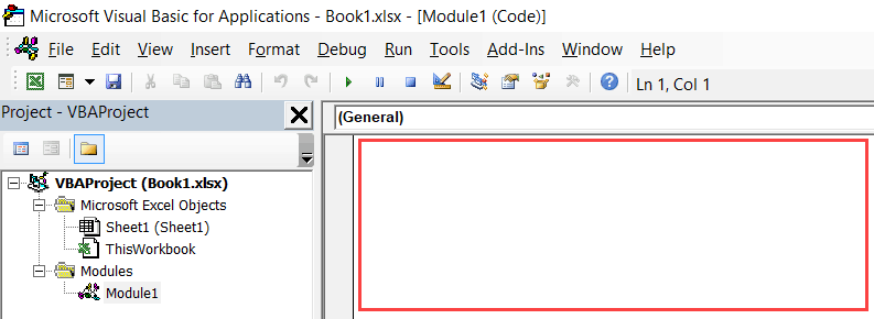
Excel has a VBA backend called the VBA editor. You need to copy and paste the code in the VB Editor module code window.
Here are the steps to do this:
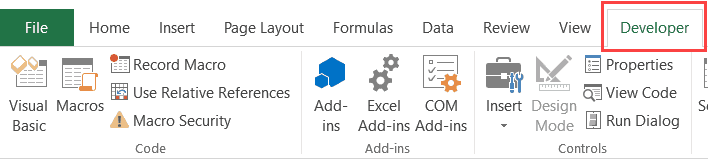
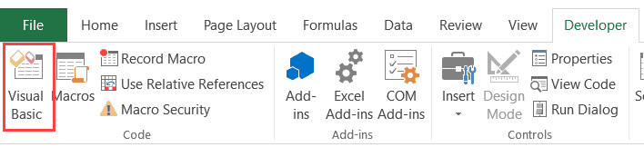
- Go to the Developer tab.

- Click on the Visual Basic option. This will open the VB editor in the backend.
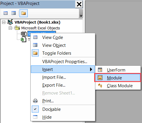
- In the Project Explorer pane in the VB Editor, right-click on any object for the workbook in which you want to insert the code. If you don’t see the Project Explorer, go to the View tab and click on Project Explorer.
- Go to Insert and click on Module. This will insert a module object for your workbook.

- Copy and paste the code in the module window.

You May Also Like the Following Excel Tutorials:
- Working with Worksheets using VBA.
- Working with Workbooks using VBA.
- Creating User-Defined Functions in Excel.
- For Next Loop in Excel VBA – A Beginner’s Guide with Examples.
- How to Use Excel VBA InStr Function (with practical EXAMPLES).
- Excel VBA Msgbox.
- How to Record a Macro in Excel.
- How to Run a Macro in Excel.
- How to Create an Add-in in Excel.
- Excel Personal Macro Workbook | Save & Use Macros in All Workbooks.
- Excel VBA Events – An Easy (and Complete) Guide.
- Excel VBA Error Handling.
- How to Sort Data in Excel using VBA (A Step-by-Step Guide).
- 24 Useful Excel Macro Examples for VBA Beginners (Ready-to-use).
Excel VBA OFFSET Function
VBA Offset function one may use to move or refer to a reference skipping a particular number of rows and columns. The arguments for this function in VBA are the same as those in the worksheet.
For example, assume you have a data set like the one below.
Now from cell A1, you want to move down four cells and select that 5th cell, the A5 cell.
Similarly, if you want to move two rows down from the A1 cell and two columns to the right, select that cell, i.e., the C2 cell.
In these cases, the OFFSET function is very helpful. Especially in VBA OFFSET, the function is just phenomenal.
Table of contents
- Excel VBA OFFSET Function
- OFFSET is Used with Range Object in Excel VBA
- Syntax of OFFSET in VBA Excel
- Examples
- Example #1
- Example #2
- Example #3
- Example #4
- Things to Remember
- Recommended Articles
OFFSET is Used with Range Object in Excel VBA
In VBA, we cannot directly enter the word OFFSET. Instead, we need to use the VBA RANGE objectRange is a property in VBA that helps specify a particular cell, a range of cells, a row, a column, or a three-dimensional range. In the context of the Excel worksheet, the VBA range object includes a single cell or multiple cells spread across various rows and columns.read more first. Then, from that range object, we can use the OFFSET property.
In Excel, the range is nothing but a cell or range of the cell. Since OFFSET refers to cells, we need to use the object RANGE first, and then we can use the OFFSET method.
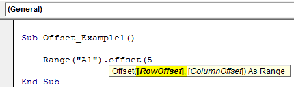
Syntax of OFFSET in VBA Excel
![]()
- Row Offset: How many rows do you want to offset from the selected cell? Here the selected cell is A1, i.e., Range (“A1”).
- Column Offset: How many columns do you want to offset from the selected cell? Here, the selected cell is A,1, i.e., Range (“A1”).
Examples
You can download this VBA OFFSET Template here – VBA OFFSET Template
Example #1
Consider the below data for demonstration.
Now, we want to select cell A6 from cell A1. But, first, start the macro and reference cell using the Range object.
Code:
Sub Offset_Example1()

    Range("A1").offset(

End Sub

Now, we want to select cell A6. Then, we want to go down 5 cells. So, enter 5 as the parameter for Row Offset.
Code:
Sub Offset_Example1()

    Range("A1").offset(5

End Sub
Since we are selecting the same column, we leave out the column part. Close the bracket, put a dot (.), and type the method “Select.”
Code:
Sub Offset_Example1()

    Range("A1").Offset(5).Select

End Sub

Now, run this code using the F5 key, or you can run it manually to select cell A6, as shown below.
Output:

Example #2
Now, take the same data, but here will also see how to use the column offset argument. Now, we want to select cell C5.
Since we want to select cell C5 firstly, we want to move down four cells and take the right two columns to reach cell C5. The below code would do the job for us.
Code:
Sub Offset_Example2()

    Range("A1").Offset(4, 2).Select

End Sub

We run this code manually or using the F5 key. Then, it will select cell C5, as shown in the below screenshot.
Output:

Example #3
We have seen how to offset rows and columns. We can also select the above cells from the specified cells. For example, if you are in cell A10 and want to select the A1 cell, how do you select it?
In the case of moving down the cell, we can enter a positive number, so here in the case of moving up, we need to enter negative numbers.
From the A9 cell, we need to move up by 8 rows, i.e., -8.
Code:
Sub Offset_Example1()

    Range("A9").Offset(-8).Select

End Sub

If you run this code using the F5 key or manually run it, it will select cell A1 from the A9 cell.

Output:

Example #4
Assume you are in cell C8. From this cell, you want to select cell A10.
From the active cell, i.e., the C8 cell, we need to first move down 2 rows and move to the left by 2 columns to select cell A10.
In case of moving left to select the column, we need to specify the number is negative. So, here we need to come back by -2 columns.
Code:
Sub Offset_Example2()

    Range("C8").Offset(2, -2).Select

End Sub

Now, run this code using the F5 key or run it manually. It will select the A10 cell as shown below:
Output:

Things to Remember
- In moving up rows, we need to specify the number in negatives.
- In case of moving left to select the column, the number should be negative.
- A1 cell is the first row and first column.
- The “Active Cell” means presently selected cells.
- To select the cell using OFFSET, you need to mention “.Select.”
- To copy the cell using OFFSET, you need to mention “.Copy.”
Recommended Articles
This article has been a guide to VBA OFFSET. Here, we learn how to use VBA OFFSET Property to navigate in Excel, practical examples, and a downloadable template. Below are some useful Excel articles related to VBA:-
- Active Cell in VBA
- VBA Set
- What is OFFSET Formula in Excel?
- VBA Cells References
- VBA Format Date
Вас может заинтересовать, а как можно сдвинуться влево или вправо назад или вперед от текущей ячейки. Для этого у объекта Range есть метод Offset, который и позволяет производить подобные действия.
Sub Test()
	Dim cur_range As Range
	Set cur_range = Range("A1")
	Set cur_range = cur_range.Offset(1, 0)
	Debug.Print cur_range.Address
End Sub
А вот результат работы. Мы от текущего объекта сдвинулись влево на 1 колонку.
$A$2
Если вы хотите узнать максимальные размеры листа, то у Вас есть возможность это сделать используя UsedRange. У вас будет объект типа Range, из которого вы сможете узнать максимальную колонку или строку.
Sub Test()
	With ActiveSheet
		Dim cur_range As Range
		Set cur_range = .UsedRange
		Debug.Print cur_range.Address
	End With
End Sub
Адресовать ячейки можно и двумя цифрами по колонки и сроке. Это избавляет Вас от утомительного разбора адресов типа $A10. Так как адрес строка придеться её резать и собирать. Использования Cells(x,y) очень гибко в использовании и позволяет строить легкие циклы. Пример ниже находит на листе левый верхний угол из всех ячеек с введенными данными и в эту ячейку записывает слово.
Sub Test()
	' объект Range
	Dim cur_range As Range
	' Весь лист
	With ActiveSheet
		Set cur_range = .UsedRange
		Debug.Print cur_range.Address
		' у меня печатает $C$5:$J$48
		Dim y_min As Integer
		' минимальная колонка
		y_min = cur_range.Columns.Column
		Dim x_min As Integer
		' минимальная строка
		x_min = cur_range.Rows.Row
		Set cur_range = Range(Cells(x_min, y_min), Cells(x_min, y_min))
		cur_range = "lef up"
	End With
End Sub
Синтаксис
- Set — оператор, используемый для установки ссылки на объект, например, на диапазон
- Для каждого — оператор, используемый для прокрутки каждого элемента в коллекции
замечания
Обратите внимание, что имена переменных r , cell и другие могут быть названы, как вам нравится, но должны быть названы соответствующим образом, чтобы код был более понятным для вас и других.
Создание диапазона
Диапазон нельзя создать или заполнить так же, как строка:
Sub RangeTest()
    Dim s As String
    Dim r As Range 'Specific Type of Object, with members like Address, WrapText, AutoFill, etc.

    ' This is how we fill a String:
    s = "Hello World!"

    ' But we cannot do this for a Range:
    r = Range("A1") '//Run. Err.:  91 Object variable or With block variable not set//

    ' We have to use the Object approach, using keyword Set:
    Set r = Range("A1")
End Sub
Считается лучшей практикой, чтобы квалифицировать ваши ссылки , поэтому в дальнейшем мы будем использовать один и тот же подход.
Подробнее о создании объектных переменных (например, Range) в MSDN . Подробнее о Set Statement на MSDN .
Существуют разные способы создания одного и того же диапазона:
Sub SetRangeVariable()
    Dim ws As Worksheet
    Dim r As Range

    Set ws = ThisWorkbook.Worksheets(1) ' The first Worksheet in Workbook with this code in it

    ' These are all equivalent:
    Set r = ws.Range("A2")
    Set r = ws.Range("A" & 2)
    Set r = ws.Cells(2, 1) ' The cell in row number 2, column number 1
    Set r = ws.[A2] 'Shorthand notation of Range.
    Set r = Range("NamedRangeInA2") 'If the cell A2 is named NamedRangeInA2. Note, that this is Sheet independent.
    Set r = ws.Range("A1").Offset(1, 0) ' The cell that is 1 row and 0 columns away from A1
    Set r = ws.Range("A1").Cells(2,1) ' Similar to Offset. You can "go outside" the original Range.

    Set r = ws.Range("A1:A5").Cells(2) 'Second cell in bigger Range.
    Set r = ws.Range("A1:A5").Item(2) 'Second cell in bigger Range.
    Set r = ws.Range("A1:A5")(2) 'Second cell in bigger Range.
End Sub
Обратите внимание на пример, что ячейки (2, 1) эквивалентны диапазону («A2»). Это происходит потому, что Cells возвращает объект Range.
Некоторые источники: Chip Pearson-Cells Within Ranges ; Объект диапазона MSDN ; John Walkenback — ссылка на диапазоны в коде VBA .
Также обратите внимание, что в любом случае, когда число используется в объявлении диапазона, а сам номер находится вне кавычек, например Range («A» & 2), вы можете поменять это число на переменную, содержащую целое число / долго. Например:
Sub RangeIteration()
    Dim wb As Workbook, ws As Worksheet
    Dim r As Range

    Set wb = ThisWorkbook
    Set ws = wb.Worksheets(1)

    For i = 1 To 10
        Set r = ws.Range("A" & i)
        ' When i = 1, the result will be Range("A1")
        ' When i = 2, the result will be Range("A2")
        ' etc.
        ' Proof:
        Debug.Print r.Address
    Next i
End Sub
Если вы используете двойные циклы, ячейки лучше:
Sub RangeIteration2()
    Dim wb As Workbook, ws As Worksheet
    Dim r As Range

    Set wb = ThisWorkbook
    Set ws = wb.Worksheets(1)

    For i = 1 To 10
        For j = 1 To 10
            Set r = ws.Cells(i, j)
            ' When i = 1 and j = 1, the result will be Range("A1")
            ' When i = 2 and j = 1, the result will be Range("A2")
            ' When i = 1 and j = 2, the result will be Range("B1")
            ' etc.
            ' Proof:
            Debug.Print r.Address
        Next j
    Next i
End Sub
Способы обращения к одной ячейке
Самый простой способ ссылаться на одну ячейку на текущем листе Excel — это просто вставить форму А1 в ссылку в квадратных скобках:
[a3] = "Hello!"
Обратите внимание, что квадратные скобки — это просто удобный синтаксический сахар для метода Evaluate объекта Application , так что технически это идентично следующему коду:
Application.Evaluate("a3") = "Hello!"
Вы также можете вызвать метод Cells который принимает строку и столбец и возвращает ссылку на ячейку.
Cells(3, 1).Formula = "=A1+A2"
Помните, что всякий раз, когда вы передаете строку и столбец в Excel из VBA, строка всегда первая, за ней следует столбец, что запутывает, потому что это противоположно общей нотации A1 где сначала отображается столбец.
В обоих этих примерах мы не указали рабочий лист, поэтому Excel будет использовать активный лист (лист, который находится впереди в пользовательском интерфейсе). Вы можете указать активный лист явно:
ActiveSheet.Cells(3, 1).Formula = "=SUM(A1:A2)"
Или вы можете указать имя определенного листа:
Sheets("Sheet2").Cells(3, 1).Formula = "=SUM(A1:A2)"
Существует множество методов, которые можно использовать для перехода от одного диапазона к другому. Например, метод Rows может использоваться для доступа к отдельным строкам любого диапазона, и метод Cells может использоваться для доступа к отдельным ячейкам строки или столбца, поэтому следующий код относится к ячейке C1:
ActiveSheet.Rows(1).Cells(3).Formula = "hi!"
Сохранение ссылки на ячейку переменной
Чтобы сохранить ссылку на ячейку в переменной, вы должны использовать синтаксис Set , например:
Dim R as Range
Set R = ActiveSheet.Cells(3, 1)
потом…
R.Font.Color = RGB(255, 0, 0)
Почему требуется ключевое слово Set ? Set указывает Visual Basic, что значение в правой части = означает объект.
Смещение недвижимости
- Смещение (строки, столбцы) — оператор, используемый для статической ссылки на другую точку из текущей ячейки. Часто используется в циклах. Следует понимать, что положительные числа в разделе строк перемещаются вправо, поскольку негативы перемещаются влево. С положительными позициями столбцов вниз и негативы двигаются вверх.
т.е.
Private Sub this()
    ThisWorkbook.Sheets("Sheet1").Range("A1").Offset(1, 1).Select
    ThisWorkbook.Sheets("Sheet1").Range("A1").Offset(1, 1).Value = "New Value"
    ActiveCell.Offset(-1, -1).Value = ActiveCell.Value
    ActiveCell.Value = vbNullString
End Sub
Этот код выбирает B2, помещает туда новую строку, затем перемещает эту строку обратно в A1 после очистки B2.
Как перемещать диапазоны (по горизонтали по вертикали и наоборот)
Sub TransposeRangeValues()
    Dim TmpArray() As Variant, FromRange as Range, ToRange as Range

    set FromRange = Sheets("Sheet1").Range("a1:a12")         'Worksheets(1).Range("a1:p1")
    set ToRange = ThisWorkbook.Sheets("Sheet1").Range("a1")  'ThisWorkbook.Sheets("Sheet1").Range("a1")

    TmpArray = Application.Transpose(FromRange.Value)
    FromRange.Clear
    ToRange.Resize(FromRange.Columns.Count,FromRange.Rows.Count).Value2 = TmpArray
End Sub
Примечание. Copy / PasteSpecial также имеет параметр «Вставить транспонирование», который также обновляет формулы транспонированных ячеек.
|
0 / 0 / 0 Регистрация: 09.01.2013 Сообщений: 13 |
|
|
1 |
|
|
09.01.2013, 18:33. Показов 17999. Ответов 12
Добрый день. Делаю очень большой древовидный список в Excel. Часто приходится перетаскивать ячейку на 1 вправо. A1 -> A2, B3->B4 и т.д. Можно ли как-то делать это действие горячими клавишами? Наверное требуется макрос. Если кто подскажет такой — буду очень благодарен. Спасибо.
0 |

|
5468 / 1148 / 50 Регистрация: 15.09.2012 Сообщений: 3,514 |
|
|
09.01.2013, 19:18 |
2 |
|
lehachgtop, выложите книгу Excel с примерными данными и поясните, что нужно сделать.
0 |
|
0 / 0 / 0 Регистрация: 09.01.2013 Сообщений: 13 |
|
|
09.01.2013, 19:58 [ТС] |
3 |
|
перетаскивать ячейку на 1 вправо. A1 -> A2, B3->B4 Ошибся. A1 -> B2, B3 -> C3 и т.д. Сделал примерную книгу. Если бы можно было одной клавишей (или простой комбинацией клавиш) перемещать содержимое ячейки в ячейку соседнего столбца справа — это в разы бы ускорило работу.
0 |

|
Скрипт 5468 / 1148 / 50 Регистрация: 15.09.2012 Сообщений: 3,514 |
||||
|
09.01.2013, 20:07 |
4 |
|||
|
lehachgtop, вот по такому принципу можно перемещать данные из активной ячейки в ячейку, находящуюся справа:
А как вызывать этот макрос — вам решать. Можно сочетание клавиш сделать. Ещё у листа есть события, например, при двойном клике по ячейке можно вызывать макрос.
1 |
|
0 / 0 / 0 Регистрация: 09.01.2013 Сообщений: 13 |
|
|
09.01.2013, 21:02 [ТС] |
5 |
|
А можно с помощью макроса сделать выделение ячеек (фон)? Например я выделил 6 ячеек, жму клавиши, и макрос выделяет заданным цветом фон.
0 |
|
Igor_Tr 4377 / 661 / 36 Регистрация: 17.01.2010 Сообщений: 2,134 |
||||
|
09.01.2013, 21:22 |
6 |
|||
|
Можно, конечно! Но зачем с помощью макроса, и жать клавиши?
Осталось Вам только продумать, как программа, по каким критериям, будет определять ячейки под заливку.
0 |
|
0 / 0 / 0 Регистрация: 09.01.2013 Сообщений: 13 |
|
|
09.01.2013, 22:06 [ТС] |
7 |
|
как программа, по каким критериям, будет определять ячейки под заливку. Но это должен определять я вручную. Быстрее всего — с горячими клавишами.
0 |
|
Igor_Tr 4377 / 661 / 36 Регистрация: 17.01.2010 Сообщений: 2,134 |
||||
|
10.01.2013, 00:17 |
8 |
|||
|
Хорошо, давайте по другому. Чем Вы будете руководствоваться при выделении вручную? Наличием текста?, символов?, цифр?, комбинациями? Вот это и научите железяку. Она послушная. Например, если у Вас в ячейке встречаеться число 2 — закрасить! немедленно!
А вобще есть еще много способов сделать это-же. Добавлено через 16 минут
0 |
|
0 / 0 / 0 Регистрация: 09.01.2013 Сообщений: 13 |
|
|
10.01.2013, 08:54 [ТС] |
9 |
|
Чем Вы будете руководствоваться при выделении вручную? Наличием текста?, символов?, цифр?, комбинациями? Вот это и научите железяку. Мне придется выделять исключительно вручную. Надо выделять похожие по смыслу, но разные по написанию слова: велик, байк и велосипед. Как-то автоматизировать это невозможно. Поэтому я по-прежнему хочу выделять нажатием клавиши (комбинацией клавиш). Наверное для этого нужен макрос. Прошу помочь.
0 |
|
Скрипт 5468 / 1148 / 50 Регистрация: 15.09.2012 Сообщений: 3,514 |
||||
|
10.01.2013, 09:15 |
10 |
|||
|
Код, который делают заливку у выделенных ячеек: Кликните здесь для просмотра всего текста
0 |
|
Igor_Tr 4377 / 661 / 36 Регистрация: 17.01.2010 Сообщений: 2,134 |
||||||||
|
10.01.2013, 14:43 |
11 |
|||||||
|
Мне кажется, что можно. Велик, байк и велосипед — а что у них общего? Все это средства передвижения, которые можно обьеденить в группу, например RemedForMovement. Создайте массив — и вперед. Главное — экспериментируйте, иначе Вам и святой Франциск не поможет. Но если Вам нравится в ручную — тоже не плохо. Ручная работа ценится во всем мире. Добавлено через 2 часа 12 минут
Из этого макроса запускаем заливку (а стоило это трудов? Не проще было выделить и выбрать цвет на панели?)
К кнопке еще можно добавить розочки, бантики… и все это группировать. По вкусу
1 |

|
0 / 0 / 0 Регистрация: 05.11.2015 Сообщений: 11 |
|
|
17.07.2013, 16:18 |
12 |
|
Ребят подскажите пожалуйста, а как написать перенос каждой второй строки столбца А в столбец Б??чтобы можно было сделать это действие по 100 позициям
0 |
|
Igor_Tr 4377 / 661 / 36 Регистрация: 17.01.2010 Сообщений: 2,134 |
||||
|
17.07.2013, 16:36 |
13 |
|||
|
Как-будто кол-во позиций не имеет очень значение. Добавлено через 12 минут
3 |
") Больше значит, в каком виде они должны быть в столбце В. С пропусками, или все нужные подряд?
Больше значит, в каком виде они должны быть в столбце В. С пропусками, или все нужные подряд?Return to VBA Code Examples
The Offset Property is used to return a cell or a range, that is relative to a specified input cell or range.
Using Offset with the Range Object
You could use the following code with the Range object and the Offset property to select cell B2, if cell A1 is the input range:
Range("A1").Offset(1, 1).SelectThe result is:
Notice the syntax:
Range.Offset(RowOffset, ColumnOffset)
Positive integers tells Offset to move down and to the right. Negative integers move up and to the left.
The Offset property always starts counting from the top left cell of the input cell or range.
Using Offset with the Cells Object
You could use the following code with the Cells object and the Offset property to select cell C3 if cell D4 is the input range:
Cells(4, 4).Offset(-1, -1).Select
Selecting a Group of Cells
You can also select a group of cells using the Offset property. The following code will select the range which is 7 rows below and 3 columns to the right of input Range(“A1:A5”):
Range("A1:A5").Offset(7, 3).SelectRange(“D8:D12”) is selected:
VBA Coding Made Easy
Stop searching for VBA code online. Learn more about AutoMacro — A VBA Code Builder that allows beginners to code procedures from scratch with minimal coding knowledge and with many time-saving features for all users!

Learn More!