Vba excel как выбрать ячейку - Word и Excel - помощь в работе с программами

Download Article

This wikiHow teaches you how to start using Visual Basic procedures to select data in Microsoft Excel. As long as you’re familiar with basic VB scripting and using more advanced features of Excel, you’ll find the selection process pretty straight-forward.

1
Select one cell on the current worksheet. Let’s say you want to select cell E6 with Visual Basic. You can do this with either of the following options:^[1]
```
ActiveSheet.Cells(6, 5).Select
```
```
ActiveSheet.Range("E6").Select
```
2
Select one cell on a different worksheet in the same workbook. Let’s say our example cell, E6, is on a sheet called Sheet2. You can use either of the following options to select it:
```
Application.Goto ActiveWorkbook.Sheets("Sheet2").Cells(6, 5)
```
```
Application.Goto (ActiveWorkbook.Sheets("Sheet2").Range("E6"))
```
Advertisement
3
Select one cell on a worksheet in a different workbook. Let’s say you want to select a cell from Sheet1 in a workbook called BOOK2.XLS. Either of these two options should do the trick:
```
Application.Goto Workbooks("BOOK2.XLS").Sheets("Sheet1").Cells(2,1)
```
```
Application.Goto Workbooks("BOOK2.XLS").Sheets("Sheet1").Range("A2")
```
4
Select a cell relative to another cell. You can use VB to select a cell based on its location relative to the active (or a different) cell. Just be sure the cell exists to avoid errors. Here’s how to use :
- Select the cell three rows below and four columns to the left of the active cell:
```
ActiveCell.Offset(3, -4).Select
```
- Select the cell five rows below and four columns to the right of cell C7:
```
ActiveSheet.Cells(7, 3).Offset(5, 4).Select
```

1
Select a range of cells on the active worksheet. If you wanted to select cells C1:D6 on the current sheet, you can enter any of the following three examples:
```
ActiveSheet.Range(Cells(1, 3), Cells(6, 4)).Select
```
```
ActiveSheet.Range("C1:D6").Select
```
```
ActiveSheet.Range("C1", "D6").Select
```
2
Select a range from another worksheet in the same workbook. You could use either of these examples to select cells C3:E11 on a sheet called Sheet3:
```
Application.Goto ActiveWorkbook.Sheets("Sheet3").Range("C3:E11")
```
```
Application.Goto ActiveWorkbook.Sheets("Sheet3").Range("C3", "E11")
```
3
Select a range of cells from a worksheet in a different workbook. Both of these examples would select cells E12:F12 on Sheet1 of a workbook called BOOK2.XLS:
```
Application.Goto Workbooks("BOOK2.XLS").Sheets("Sheet1").Range("E12:F12")
```
```
Application.Goto Workbooks("BOOK2.XLS").Sheets("Sheet1").Range("E12", "F12")
```
4
Select a named range. If you’ve assigned a name to a range of cells, you’d use the same syntax as steps 4-6, but you’d replace the range address (e.g., «E12», «F12») with the range’s name (e.g., «Sales»). Here are some examples:
- On the active sheet:
```
ActiveSheet.Range("Sales").Select
```
- Different sheet of same workbook:
```
Application.Goto ActiveWorkbook.Sheets("Sheet3").Range("Sales")
```
- Different workbook:
```
Application.Goto Workbooks("BOOK2.XLS").Sheets("Sheet1").Range("Sales")
```
5
Select a range relative to a named range. The syntax varies depending on the named range’s location and whether you want to adjust the size of the new range.
- If the range you want to select is the same size as one called Test5 but is shifted four rows down and three columns to the right, you’d use:
```
ActiveSheet.Range("Test5").Offset(4, 3).Select
```
- If the range is on Sheet3 of the same workbook, activate that worksheet first, and then select the range like this:
```
Sheets("Sheet3").Activate ActiveSheet.Range("Test").Offset(4, 3).Select
```
6
Select a range and resize the selection. You can increase the size of a selected range if you need to. If you wanted to select a range called Database’ and then increase its size by 5 rows, you’d use this syntax:
```
Range("Database").Select Selection.Resize(Selection.Rows.Count + 5, _Selection.Columns.Count).Select
```
7
Select the union of two named ranges. If you have two overlapping named ranges, you can use VB to select the cells in that overlapping area (called the «union»). The limitation is that you can only do this on the active sheet. Let’s say you want to select the union of a range called Great and one called Terrible:
- ```
Application.Union(Range("Great"), Range("Terrible")).Select
```
- If you want to select the intersection of two named ranges instead of the overlapping area, just replace Application.Union with Application.Intersect.

1

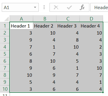
Use this example data for the examples in this method. This chart full of example data, courtesy of Microsoft, will help you visualize how the examples behave:^[2]

A1: Name B1: Sales C1: Quantity

A2: a B2: $10 C2: 5

A3: b B3: C3: 10

A4: c B4: $10 C4: 5

A5: B5: C5:

A6: Total B6: $20 C6: 20
2
Select the last cell at the bottom of a contiguous column. The following example will select cell A4:
```
ActiveSheet.Range("A1").End(xlDown).Select
```
3
Select the first blank cell below a column of contiguous cells. The following example will select A5 based on the chart above:
```
ActiveSheet.Range("A1").End(xlDown).Offset(1,0).Select
```
4
Select a range of continuous cells in a column. Both of the following examples will select the range A1:A4:
```
ActiveSheet.Range("A1", ActiveSheet.Range("a1").End(xlDown)).Select
```
```
ActiveSheet.Range("A1:" & ActiveSheet.Range("A1"). End(xlDown).Address).Select
```
5
Select a whole range of non-contiguous cells in a column. Using the data table at the top of this method, both of the following examples will select A1:A6:
```
ActiveSheet.Range("A1",ActiveSheet.Range("A65536").End(xlUp)).Select
```
```
ActiveSheet.Range("A1",ActiveSheet.Range("A65536").End(xlUp)).Select
```

Ask a Question

200 characters left

Include your email address to get a message when this question is answered.

Submit

Video

The «ActiveSheet» and «ActiveWorkbook» properties can usually be omitted if the active sheet and/or workbook(s) are implied.

Thanks for submitting a tip for review!

About This Article

Article SummaryX

1. Use ActiveSheet.Range(«E6»).Select to select E6 on the active sheet.
2. Use Application.Goto (ActiveWorkbook.Sheets(«Sheet2»).Range(«E6»)) to select E6 on Sheet2.
3. Add Workbooks(«BOOK2.XLS») to the last step to specify that the sheet is in BOOK2.XLS.

Did this summary help you?

Thanks to all authors for creating a page that has been read 167,714 times.

Is this article up to date?

Источник

Всё о работе с ячейками в Excel-VBA: обращение, перебор, удаление, вставка, скрытие, смена имени.

Содержание:

Table of Contents:

Что такое ячейка Excel?
Способы обращения к ячейкам
- Выбор и активация
- Получение и изменение значений ячеек
  - Ячейки открытой книги
  - Ячейки закрытой книги
- Перебор ячеек
- Перебор в произвольном диапазоне
Свойства и методы ячеек
- Имя ячейки
- Адрес ячейки
- Размеры ячейки
Запуск макроса активацией ячейки

2 нюанса:

Я почти везде стараюсь использовать ThisWorkbook (а не, например, ActiveWorkbook) для обращения к текущей книге, в которой написан этот код (считаю это наиболее безопасным для новичков способом обращения к книгам, чтобы случайно не внести изменения в другие книги). Для экспериментов можете вставлять этот код в модули, коды книги, либо листа, и он будет работать только в пределах этой книги.
Я использую английский эксель и у меня по стандарту листы называются Sheet1, Sheet2 и т.д. Если вы работаете в русском экселе, то замените Thisworkbook.Sheets(«Sheet1») на Thisworkbook.Sheets(«Лист1»). Если этого не сделать, то вы получите ошибку в связи с тем, что пытаетесь обратиться к несуществующему объекту. Можно также заменить на Thisworkbook.Sheets(1), но это менее безопасно.

Что такое ячейка Excel?

В большинстве мест пишут: «элемент, образованный пересечением столбца и строки». Это определение полезно для людей, которые не знакомы с понятием «таблица». Для того, чтобы понять чем на самом деле является ячейка Excel, необходимо заглянуть в объектную модель Excel. При этом определения объектов «ряд», «столбец» и «ячейка» будут отличаться в зависимости от того, как мы работаем с файлом.

Объекты в Excel-VBA. Пока мы работаем в Excel без углубления в VBA определение ячейки как «пересечения» строк и столбцов нам вполне хватает, но если мы решаем как-то автоматизировать процесс в VBA, то о нём лучше забыть и просто воспринимать лист как «мешок» ячеек, с каждой из которых VBA позволяет работать как минимум тремя способами:

по цифровым координатам (ряд, столбец),
по адресам формата А1, B2 и т.д. (сценарий целесообразности данного способа обращения в VBA мне сложно представить)
по уникальному имени (во втором и третьем вариантах мы будем иметь дело не совсем с ячейкой, а с объектом VBA range, который может состоять из одной или нескольких ячеек). Функции и методы объектов Cells и Range отличаются. Новичкам я бы порекомендовал работать с ячейками VBA только с помощью Cells и по их цифровым координатам и использовать Range только по необходимости.

Все три способа обращения описаны далее

Как это хранится на диске и как с этим работать вне Excel? С точки зрения хранения и обработки вне Excel и VBA. Сделать это можно, например, сменив расширение файла с .xls(x) на .zip и открыв этот архив.

Пример содержимого файла Excel:

Далее xl -> worksheets и мы видим файл листа

Содержимое файла:

То же, но более наглядно:

<?xml version="1.0" encoding="UTF-8" standalone="yes"?>
<worksheet xmlns="http://schemas.openxmlformats.org/spreadsheetml/2006/main" xmlns:r="http://schemas.openxmlformats.org/officeDocument/2006/relationships" xmlns:mc="http://schemas.openxmlformats.org/markup-compatibility/2006" mc:Ignorable="x14ac xr xr2 xr3" xmlns:x14ac="http://schemas.microsoft.com/office/spreadsheetml/2009/9/ac" xmlns:xr="http://schemas.microsoft.com/office/spreadsheetml/2014/revision" xmlns:xr2="http://schemas.microsoft.com/office/spreadsheetml/2015/revision2" xmlns:xr3="http://schemas.microsoft.com/office/spreadsheetml/2016/revision3" xr:uid="{00000000-0001-0000-0000-000000000000}">
	<dimension ref="B2:F6"/>
	<sheetViews>
		<sheetView tabSelected="1" workbookViewId="0">
			<selection activeCell="D12" sqref="D12"/>
		</sheetView>
	</sheetViews>
	<sheetFormatPr defaultRowHeight="14.4" x14ac:dyDescent="0.3"/>
	<sheetData>
		<row r="2" spans="2:6" x14ac:dyDescent="0.3">
			<c r="B2" t="s">
				<v>0</v>
			</c>
		</row>
		<row r="3" spans="2:6" x14ac:dyDescent="0.3">
			<c r="C3" t="s">
				<v>1</v>
			</c>
		</row>
		<row r="4" spans="2:6" x14ac:dyDescent="0.3">
			<c r="D4" t="s">
				<v>2</v>
			</c>
		</row>
		<row r="5" spans="2:6" x14ac:dyDescent="0.3">
			<c r="E5" t="s">
				<v>0</v></c>
		</row>
		<row r="6" spans="2:6" x14ac:dyDescent="0.3">
			<c r="F6" t="s"><v>3</v>
		</c></row>
	</sheetData>
	<pageMargins left="0.7" right="0.7" top="0.75" bottom="0.75" header="0.3" footer="0.3"/>
</worksheet>

Как мы видим, в структуре объектной модели нет никаких «пересечений». Строго говоря рабочая книга — это архив структурированных данных в формате XML. При этом в каждую «строку» входит «столбец», и в нём в свою очередь прописан номер значения данного столбца, по которому оно подтягивается из другого XML файла при открытии книги для экономии места за счёт отсутствия повторяющихся значений. Почему это важно. Если мы захотим написать какой-то обработчик таких файлов, который будет напрямую редактировать данные в этих XML, то ориентироваться надо на такую модель и структуру данных. И правильное определение будет примерно таким: ячейка — это объект внутри столбца, который в свою очередь находится внутри строки в файле xml, в котором хранятся данные о содержимом листа.

Способы обращения к ячейкам

Выбор и активация

Почти во всех случаях можно и стоит избегать использования методов Select и Activate. На это есть две причины:

Это лишь имитация действий пользователя, которая замедляет выполнение программы. Работать с объектами книги можно напрямую без использования методов Select и Activate.
Это усложняет код и может приводить к неожиданным последствиям. Каждый раз перед использованием Select необходимо помнить, какие ещё объекты были выбраны до этого и не забывать при необходимости снимать выбор. Либо, например, в случае использования метода Select в самом начале программы может быть выбрано два листа вместо одного потому что пользователь запустил программу, выбрав другой лист.

Можно выбирать и активировать книги, листы, ячейки, фигуры, диаграммы, срезы, таблицы и т.д.

Отменить выбор ячеек можно методом Unselect:

Selection.Unselect

Отличие выбора от активации — активировать можно только один объект из раннее выбранных. Выбрать можно несколько объектов.

Если вы записали и редактируете код макроса, то лучше всего заменить Select и Activate на конструкцию With … End With. Например, предположим, что мы записали вот такой макрос:

Sub Macro1()
' Macro1 Macro
    Range("F4:F10,H6:H10").Select 'выбрали два несмежных диапазона зажав ctrl
    Range("H6").Activate          'показывает только то, что я начал выбирать второй диапазон с этой ячейки (она осталась белой). Это действие ни на что не влияет
    With Selection.Interior       
        .Pattern = xlSolid
        .PatternColorIndex = xlAutomatic
        .Color = 65535            'залили желтым цветом, нажав на кнопку заливки на верхней панели
        .TintAndShade = 0
        .PatternTintAndShade = 0
    End With
End Sub

Почему макрос записался таким неэффективным образом? Потому что в каждый момент времени (в каждой строке) программа не знает, что вы будете делать дальше. Поэтому в записи выбор ячеек и действия с ними — это два отдельных действия. Этот код лучше всего оптимизировать (особенно если вы хотите скопировать его внутрь какого-нибудь цикла, который должен будет исполняться много раз и перебирать много объектов). Например, так:

Sub Macro11()
'
' Macro1 Macro
    Range("F4:F10,H6:H10").Select '1. смотрим, что за объект выбран (что идёт до .Select)
    Range("H6").Activate
    With Selection.Interior       '2. понимаем, что у выбранного объекта есть свойство interior, с которым далее идёт работа
        .Pattern = xlSolid
        .PatternColorIndex = xlAutomatic
        .Color = 65535
        .TintAndShade = 0
        .PatternTintAndShade = 0
    End With
End Sub



Sub Optimized_Macro()
    With Range("F4:F10,H6:H10").Interior '3. переносим объект напрямую в конструкцию With вместо Selection
' ////// Здесь я для надёжности прописал бы ещё Thisworkbook.Sheet("ИмяЛиста") перед Range,
' ////// чтобы минимизировать риск любых случайных изменений других листов и книг
' ////// With Thisworkbook.Sheet("ИмяЛиста").Range("F4:F10,H6:H10").Interior
        .Pattern = xlSolid               '4. полностью копируем всё, что было записано рекордером внутрь блока with
        .PatternColorIndex = xlAutomatic
        .Color = 55555                   '5. здесь я поменял цвет на зеленый, чтобы было видно, работает ли код при поочерёдном запуске двух макросов
        .TintAndShade = 0
        .PatternTintAndShade = 0
    End With
End Sub

Пример сценария, когда использование Select и Activate оправдано:

Допустим, мы хотим, чтобы во время исполнения программы мы одновременно изменяли несколько листов одним действием и пользователь видел какой-то определённый лист. Это можно сделать примерно так:

Sub Select_Activate_is_OK()
Thisworkbook.Worksheets(Array("Sheet1", "Sheet3")).Select 'Выбираем несколько листов по именам
Thisworkbook.Worksheets("Sheet3").Activate 'Показываем пользователю третий лист
'Далее все действия с выбранными ячейками через Select будут одновременно вносить изменения в оба выбранных листа

'Допустим, что тут мы решили покрасить те же два диапазона:
Range("F4:F10,H6:H10").Select
    Range("H6").Activate
    With Selection.Interior       
        .Pattern = xlSolid
        .PatternColorIndex = xlAutomatic
        .Color = 65535
        .TintAndShade = 0
        .PatternTintAndShade = 0
    End With

End Sub

Единственной причиной использовать этот код по моему мнению может быть желание зачем-то показать пользователю определённую страницу книги в какой-то момент исполнения программы. С точки зрения обработки объектов, опять же, эти действия лишние.

Получение и изменение значений ячеек

Значение ячеек можно получать/изменять с помощью свойства value.

'Если нужно прочитать / записать значение ячейки, то используется свойство Value
a = ThisWorkbook.Sheets("Sheet1").Cells (1,1).Value 'записать значение ячейки А1 листа "Sheet1" в переменную "a"
ThisWorkbook.Sheets("Sheet1").Cells (1,1).Value = 1  'задать значение ячейки А1 (первый ряд, первый столбец) листа "Sheet1"

'Если нужно прочитать текст как есть (с форматированием), то можно использовать свойство .text:
ThisWorkbook.Sheets("Sheet1").Cells (1,1).Text = "1" 
a = ThisWorkbook.Sheets("Sheet1").Cells (1,1).Text

'Когда проявится разница:
'Например, если мы считываем дату в формате "31 декабря 2021 г.", хранящуюся как дата
a = ThisWorkbook.Sheets("Sheet1").Cells (1,1).Value 'эапишет как "31.12.2021"
a = ThisWorkbook.Sheets("Sheet1").Cells (1,1).Text  'запишет как "31 декабря 2021 г."

Ячейки открытой книги

К ячейкам можно обращаться:

'В книге, в которой хранится макрос (на каком-то из листов, либо в отдельном модуле или форме)
ThisWorkbook.Sheets("Sheet1").Cells(1,1).Value        'По номерам строки и столбца
ThisWorkbook.Sheets("Sheet1").Cells(1,"A").Value      'По номерам строки и букве столбца
ThisWorkbook.Sheets("Sheet1").Range("A1").Value       'По адресу - вариант 1
ThisWorkbook.Sheets("Sheet1").[A1].Value              'По адресу - вариант 2
ThisWorkbook.Sheets("Sheet1").Range("CellName").Value 'По имени ячейки (для этого ей предварительно нужно его присвоить)

'Те же действия, но с использованием полного названия рабочей книги (книга должна быть открыта)
Workbooks("workbook.xlsm").Sheets("Sheet1").Cells(1,1).Value 'По номерам строки и столбца
Workbooks("workbook.xlsm").Sheets("Sheet1").Cells(1,"A").Value                'По номерам строки и букве столбца
Workbooks("workbook.xlsm").Sheets("Sheet1").Range("A1").Value                 'По адресу - вариант 1
Workbooks("workbook.xlsm").Sheets("Sheet1").[A1].Value                        'По адресу - вариант 2
Workbooks("workbook.xlsm").Sheets("Sheet1").Range("CellName").Value           'По имени ячейки (для этого ей предварительно нужно его присвоить)

Ячейки закрытой книги

Если нужно достать или изменить данные в другой закрытой книге, то необходимо прописать открытие и закрытие книги. Непосредственно работать с закрытой книгой не получится, потому что данные в ней хранятся отдельно от структуры и при открытии Excel каждый раз производит расстановку значений по соответствующим «слотам» в структуре. Подробнее о том, как хранятся данные в xlsx см выше.

Workbooks.Open Filename:="С:closed_workbook.xlsx"    'открыть книгу (она становится активной)
a = ActiveWorkbook.Sheets("Sheet1").Cells(1,1).Value  'достать значение ячейки 1,1
ActiveWorkbook.Close False                            'закрыть книгу (False => без сохранения)

Скачать пример, в котором можно посмотреть, как доставать и как записывать значения в закрытую книгу.

Код из файла:

Option Explicit
Sub get_value_from_closed_wb() 'достать значение из закрытой книги
Dim a, wb_path, wsh As String
wb_path = ThisWorkbook.Sheets("Sheet1").Cells(2, 3).Value 'get path to workbook from sheet1
wsh = ThisWorkbook.Sheets("Sheet1").Cells(3, 3).Value
Workbooks.Open Filename:=wb_path
a = ActiveWorkbook.Sheets(wsh).Cells(3, 3).Value
ActiveWorkbook.Close False
ThisWorkbook.Sheets("Sheet1").Cells(4, 3).Value = a
End Sub

Sub record_value_to_closed_wb() 'записать значение в закрытую книгу
Dim wb_path, b, wsh As String
wsh = ThisWorkbook.Sheets("Sheet1").Cells(3, 3).Value
wb_path = ThisWorkbook.Sheets("Sheet1").Cells(2, 3).Value 'get path to workbook from sheet1
b = ThisWorkbook.Sheets("Sheet1").Cells(5, 3).Value 'get value to record in the target workbook
Workbooks.Open Filename:=wb_path
ActiveWorkbook.Sheets(wsh).Cells(4, 4).Value = b 'add new value to cell D4 of the target workbook
ActiveWorkbook.Close True
End Sub

Перебор ячеек

Перебор в произвольном диапазоне

Скачать файл со всеми примерами

Пройтись по всем ячейкам в нужном диапазоне можно разными способами. Основные:

Цикл For Each. Пример:
```
Sub iterate_over_cells()

For Each c In ThisWorkbook.Sheets("Sheet1").Range("B2:D4").Cells
MsgBox (c)
Next c

End Sub
```
Этот цикл выведет в виде сообщений значения ячеек в диапазоне B2:D4 по порядку по строкам слева направо и по столбцам — сверху вниз. Данный способ можно использовать для действий, в который вам не важны номера ячеек (закрашивание, изменение форматирования, пересчёт чего-то и т.д.).

Ту же задачу можно решить с помощью двух вложенных циклов — внешний будет перебирать ряды, а вложенный — ячейки в рядах. Этот способ я использую чаще всего, потому что он позволяет получить больше контроля над исполнением: на каждой итерации цикла нам доступны координаты ячеек. Для перебора всех ячеек на листе этим методом потребуется найти последнюю заполненную ячейку. Пример кода:

Sub iterate_over_cells()

Dim cl, rw As Integer
Dim x As Variant

'перебор области 3x3
For rw = 1 To 3 ' цикл для перебора рядов 1-3

    For cl = 1 To 3 'цикл для перебора столбцов 1-3
        x = ThisWorkbook.Sheets("Sheet1").Cells(rw + 1, cl + 1).Value
        MsgBox (x)
    Next cl
Next rw



'перебор всех ячеек на листе. Последняя ячейка определена с помощью UsedRange
'LastRow = ActiveSheet.UsedRange.Row + ActiveSheet.UsedRange.Rows.Count - 1
'LastCol = ActiveSheet.UsedRange.Column + ActiveSheet.UsedRange.Columns.Count - 1
'For rw = 1 To LastRow 'цикл перебора всех рядов
'    For cl = 1 To LastCol 'цикл для перебора всех столбцов
'        Действия 
'    Next cl
'Next rw


End Sub

Если нужно перебрать все ячейки в выделенном диапазоне на активном листе, то код будет выглядеть так:
```
Sub iterate_cell_by_cell_over_selection()
    Dim ActSheet As Worksheet
    Dim SelRange As Range
    Dim cell As Range
    
 
    Set ActSheet = ActiveSheet
    Set SelRange = Selection
    
    'if we want to do it in every cell of the selected range
    For Each cell In Selection
    MsgBox (cell.Value)
    
    Next cell

End Sub
```
Данный метод подходит для интерактивных макросов, которые выполняют действия над выбранными пользователем областями.

Перебор ячеек в ряду

Sub iterate_cells_in_row()
    Dim i, RowNum, StartCell As Long
    
    RowNum = 3 'какой ряд
    StartCell = 0 ' номер начальной ячейки (минус 1, т.к. в цикле мы прибавляем i)
    
    For i = 1 To 10 ' 10 ячеек в выбранном ряду
    ThisWorkbook.Sheets("Sheet1").Cells(RowNum, i + StartCell).Value = i '(i + StartCell) добавляет 1 к номеру столбца при каждом повторении
    Next i

End Sub

Перебор ячеек в столбце

Sub iterate_cells_in_column()
    Dim i, ColNum, StartCell As Long
    
    ColNum = 3 'какой столбец
    StartCell = 0 ' номер начальной ячейки (минус 1, т.к. в цикле мы прибавляем i)
    
    For i = 1 To 10 ' 10 ячеек
    ThisWorkbook.Sheets("Sheet1").Cells(i + StartCell, ColNum).Value = i ' (i + StartCell) добавляет 1 к номеру ряда при каждом повторении
    Next i

End Sub

Свойства и методы ячеек

Имя ячейки

Присвоить новое имя можно так:

Thisworkbook.Sheets(1).Cells(1,1).name = "Новое_Имя"

Для того, чтобы сменить имя ячейки нужно сначала удалить существующее имя, а затем присвоить новое. Удалить имя можно так:

ActiveWorkbook.Names("Старое_Имя").Delete

Пример кода для переименования ячеек:

Sub rename_cell()

old_name = "Cell_Old_Name"
new_name = "Cell_New_Name"

ActiveWorkbook.Names(old_name).Delete
ThisWorkbook.Sheets(1).Cells(2, 1).Name = new_name
End Sub

Sub rename_cell_reverse()

old_name = "Cell_New_Name"
new_name = "Cell_Old_Name"

ActiveWorkbook.Names(old_name).Delete
ThisWorkbook.Sheets(1).Cells(2, 1).Name = new_name
End Sub

Адрес ячейки

Sub get_cell_address() ' вывести адрес ячейки в формате буква столбца, номер ряда
  '$A$1 style
  txt_address = ThisWorkbook.Sheets(1).Cells(3, 2).Address
  MsgBox (txt_address)
End Sub

Sub get_cell_address_R1C1()' получить адрес столбца в формате номер ряда, номер столбца
  'R1C1 style
  txt_address = ThisWorkbook.Sheets(1).Cells(3, 2).Address(ReferenceStyle:=xlR1C1)
  MsgBox (txt_address)
End Sub

  'пример функции, которая принимает 2 аргумента: название именованного диапазона и тип желаемого адреса 
  '(1- тип $A$1 2- R1C1 - номер ряда, столбца)
Function get_cell_address_by_name(str As String, address_type As Integer)
  '$A$1 style
  Select Case address_type
    Case 1
      txt_address = Range(str).Address
    Case 2
      txt_address = Range(str).Address(ReferenceStyle:=xlR1C1)
    Case Else
      txt_address = "Wrong address type selected. 1,2 available"
    End Select
  get_cell_address_by_name = txt_address
End Function

'перед запуском нужно убедиться, что в книге есть диапазон с названием, 
'адрес которого мы хотим получить, иначе будет ошибка
Sub test_function() 'запустите эту программу, чтобы увидеть, как работает функция
  x = get_cell_address_by_name("MyValue", 2)
  MsgBox (x)
End Sub

Размеры ячейки

Ширина и длина ячейки в VBA меняется, например, так:

Sub change_size()
Dim x, y As Integer
Dim w, h As Double

'получить координаты целевой ячейки
x = ThisWorkbook.Sheets("Sheet1").Cells(2, 2).Value
y = ThisWorkbook.Sheets("Sheet1").Cells(3, 2).Value

'получить желаемую ширину и высоту ячейки
w = ThisWorkbook.Sheets("Sheet1").Cells(6, 2).Value
h = ThisWorkbook.Sheets("Sheet1").Cells(7, 2).Value

'сменить высоту и ширину ячейки с координатами x,y
ThisWorkbook.Sheets("Sheet1").Cells(x, y).RowHeight = h
ThisWorkbook.Sheets("Sheet1").Cells(x, y).ColumnWidth = w


End Sub

Прочитать значения ширины и высоты ячеек можно двумя способами (однако результаты будут в разных единицах измерения). Если написать просто Cells(x,y).Width или Cells(x,y).Height, то будет получен результат в pt (привязка к размеру шрифта).

Sub get_size()
Dim x, y As Integer
'получить координаты ячейки, с которой мы будем работать
x = ThisWorkbook.Sheets("Sheet1").Cells(2, 2).Value
y = ThisWorkbook.Sheets("Sheet1").Cells(3, 2).Value

'получить длину и ширину выбранной ячейки в тех же единицах измерения, в которых мы их задавали
ThisWorkbook.Sheets("Sheet1").Cells(2, 6).Value = ThisWorkbook.Sheets("Sheet1").Cells(x, y).ColumnWidth
ThisWorkbook.Sheets("Sheet1").Cells(3, 6).Value = ThisWorkbook.Sheets("Sheet1").Cells(x, y).RowHeight

'получить длину и ширину с помощью свойств ячейки (только для чтения) в поинтах (pt)
ThisWorkbook.Sheets("Sheet1").Cells(7, 9).Value = ThisWorkbook.Sheets("Sheet1").Cells(x, y).Width
ThisWorkbook.Sheets("Sheet1").Cells(8, 9).Value = ThisWorkbook.Sheets("Sheet1").Cells(x, y).Height

End Sub

Скачать файл с примерами изменения и чтения размера ячеек

Запуск макроса активацией ячейки

Для запуска кода VBA при активации ячейки необходимо вставить в код листа нечто подобное:

3 важных момента, чтобы это работало:

1. Этот код должен быть вставлен в код листа (здесь контролируется диапазон D4)

2-3. Программа, ответственная за запуск кода при выборе ячейки, должна называться Worksheet_SelectionChange и должна принимать значение переменной Target, относящейся к триггеру SelectionChange. Другие доступные триггеры можно посмотреть в правом верхнем углу (2).

Скачать файл с базовым примером (как на картинке)

Скачать файл с расширенным примером (код ниже)

Option Explicit

Private Sub Worksheet_SelectionChange(ByVal Target As Range)

        ' имеем в виду, что триггер SelectionChange будет запускать эту Sub после каждого клика мышью (после каждого клика будет проверяться:
          '1. количество выделенных ячеек и 
          '2. не пересекается ли выбранный диапазон с заданным в этой программе диапазоном.
        ' поэтому в эту программу не стоит без необходимости писать никаких других тяжелых операций

    If Selection.Count = 1 Then 'запускаем программу только если выбрано не более 1 ячейки


    'вариант модификации - брать адрес ячейки из другой ячейки:
    'Dim CellName as String
    'CellName = Activesheet.Cells(1,1).value 'брать текстовое имя контролируемой ячейки из A1 (должно быть в формате Буква столбца + номер строки)
    'If Not Intersect(Range(CellName), Target) Is Nothing Then
    'для работы этой модификации следующую строку надо закомментировать/удалить



        If Not Intersect(Range("D4"), Target) Is Nothing Then 
        'если заданный (D4) и выбранный диапазон пересекаются 
        '(пересечение диапазонов НЕ равно Nothing)

        'можно прописать диапазон из нескольких ячеек:
        'If Not Intersect(Range("D4:E10"), Target) Is Nothing Then
        'можно прописать несколько диапазонов:
        'If Not Intersect(Range("D4:E10"), Target) Is Nothing or Not Intersect(Range("A4:A10"), Target) Is Nothing Then

            Call program 'выполняем программу
        End If
    End If
End Sub

Sub program()

MsgBox ("Program Is running") 'здесь пишем код того, что произойдёт при выборе нужной ячейки


End Sub

Источник

When working with Excel, most of your time is spent in the worksheet area – dealing with cells and ranges.

And if you want to automate your work in Excel using VBA, you need to know how to work with cells and ranges using VBA.

There are a lot of different things you can do with ranges in VBA (such as select, copy, move, edit, etc.).

So to cover this topic, I will break this tutorial into sections and show you how to work with cells and ranges in Excel VBA using examples.

Let’s get started.

All the codes I mention in this tutorial need to be placed in the VB Editor. Go to the ‘Where to Put the VBA Code‘ section to know how it works.

If you’re interested in learning VBA the easy way, check out my Online Excel VBA Training.

Selecting a Cell / Range in Excel using VBA
- Selecting a Single Cell Using VBA
- Selecting a Fix Sized Range
- Selecting a Variably Sized Range
  - Select Using CurrentRange Property
  - Select Using UsedRange Property
  - Select Using the End Property
  - Difference between Using CurrentRegion and End
Copy Cells / Ranges Using VBA
- Copying Single Cell
- Copying a Fix Sized Range
- Copying a Variable Sized Range
Assigning Ranges to Object Variables
Enter Data in the Next Empty Cell (Using Input Box)
Looping Through Cells / Ranges
Where to Put the VBA Code

Selecting a Cell / Range in Excel using VBA

To work with cells and ranges in Excel using VBA, you don’t need to select it.

In most of the cases, you are better off not selecting cells or ranges (as we will see).

Despite that, it’s important you go through this section and understand how it works. This will be crucial in your VBA learning and a lot of concepts covered here will be used throughout this tutorial.

So let’s start with a very simple example.

Selecting a Single Cell Using VBA

If you want to select a single cell in the active sheet (say A1), then you can use the below code:

Sub SelectCell()
Range("A1").Select
End Sub

The above code has the mandatory ‘Sub’ and ‘End Sub’ part, and a line of code that selects cell A1.

Range(“A1”) tells VBA the address of the cell that we want to refer to.

Select is a method of the Range object and selects the cells/range specified in the Range object. The cell references need to be enclosed in double quotes.

This code would show an error in case a chart sheet is an active sheet. A chart sheet contains charts and is not widely used. Since it doesn’t have cells/ranges in it, the above code can’t select it and would end up showing an error.

Note that since you want to select the cell in the active sheet, you just need to specify the cell address.

But if you want to select the cell in another sheet (let’s say Sheet2), you need to first activate Sheet2 and then select the cell in it.

Sub SelectCell()
Worksheets("Sheet2").Activate
Range("A1").Select
End Sub

Similarly, you can also activate a workbook, then activate a specific worksheet in it, and then select a cell.

Sub SelectCell()
Workbooks("Book2.xlsx").Worksheets("Sheet2").Activate
Range("A1").Select
End Sub

Note that when you refer to workbooks, you need to use the full name along with the file extension (.xlsx in the above code). In case the workbook has never been saved, you don’t need to use the file extension.

Now, these examples are not very useful, but you will see later in this tutorial how we can use the same concepts to copy and paste cells in Excel (using VBA).

Just as we select a cell, we can also select a range.

In case of a range, it could be a fixed size range or a variable size range.

In a fixed size range, you would know how big the range is and you can use the exact size in your VBA code. But with a variable-sized range, you have no idea how big the range is and you need to use a little bit of VBA magic.

Let’s see how to do this.

Selecting a Fix Sized Range

Here is the code that will select the range A1:D20.

Sub SelectRange()
Range("A1:D20").Select
End Sub

Another way of doing this is using the below code:

Sub SelectRange()
Range("A1", "D20").Select
End Sub

The above code takes the top-left cell address (A1) and the bottom-right cell address (D20) and selects the entire range. This technique becomes useful when you’re working with variably sized ranges (as we will see when the End property is covered later in this tutorial).

If you want the selection to happen in a different workbook or a different worksheet, then you need to tell VBA the exact names of these objects.

For example, the below code would select the range A1:D20 in Sheet2 worksheet in the Book2 workbook.

Sub SelectRange()
Workbooks("Book2.xlsx").Worksheets("Sheet1").Activate
Range("A1:D20").Select
End Sub

Now, what if you don’t know how many rows are there. What if you want to select all the cells that have a value in it.

In these cases, you need to use the methods shown in the next section (on selecting variably sized range).

Selecting a Variably Sized Range

There are different ways you can select a range of cells. The method you choose would depend on how the data is structured.

In this section, I will cover some useful techniques that are really useful when you work with ranges in VBA.

Select Using CurrentRange Property

In cases where you don’t know how many rows/columns have the data, you can use the CurrentRange property of the Range object.

The CurrentRange property covers all the contiguous filled cells in a data range.

Below is the code that will select the current region that holds cell A1.

Sub SelectCurrentRegion()
Range("A1").CurrentRegion.Select
End Sub

The above method is good when you have all data as a table without any blank rows/columns in it.

But in case you have blank rows/columns in your data, it will not select the ones after the blank rows/columns. In the image below, the CurrentRegion code selects data till row 10 as row 11 is blank.

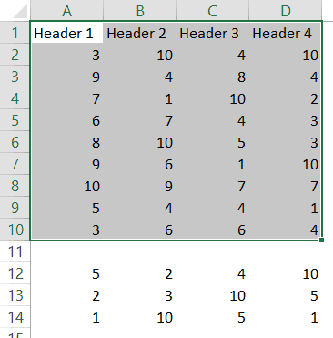
In such cases, you may want to use the UsedRange property of the Worksheet Object.

Select Using UsedRange Property

UsedRange allows you to refer to any cells that have been changed.

So the below code would select all the used cells in the active sheet.

Sub SelectUsedRegion()
ActiveSheet.UsedRange.Select
End Sub

Note that in case you have a far-off cell that has been used, it would be considered by the above code and all the cells till that used cell would be selected.

Select Using the End Property

Now, this part is really useful.

The End property allows you to select the last filled cell. This allows you to mimic the effect of Control Down/Up arrow key or Control Right/Left keys.

Let’s try and understand this using an example.

Suppose you have a dataset as shown below and you want to quickly select the last filled cells in column A.

The problem here is that data can change and you don’t know how many cells are filled. If you have to do this using keyboard, you can select cell A1, and then use Control + Down arrow key, and it will select the last filled cell in the column.

Now let’s see how to do this using VBA. This technique comes in handy when you want to quickly jump to the last filled cell in a variably-sized column

Sub GoToLastFilledCell()
Range("A1").End(xlDown).Select
End Sub

The above code would jump to the last filled cell in column A.

Similarly, you can use the End(xlToRight) to jump to the last filled cell in a row.

Sub GoToLastFilledCell()
Range("A1").End(xlToRight).Select
End Sub

Now, what if you want to select the entire column instead of jumping to the last filled cell.

You can do that using the code below:

Sub SelectFilledCells()
Range("A1", Range("A1").End(xlDown)).Select
End Sub

In the above code, we have used the first and the last reference of the cell that we need to select. No matter how many filled cells are there, the above code will select all.

Remember the example above where we selected the range A1:D20 by using the following line of code:

Range(“A1″,”D20”)

Here A1 was the top-left cell and D20 was the bottom-right cell in the range. We can use the same logic in selecting variably sized ranges. But since we don’t know the exact address of the bottom-right cell, we used the End property to get it.

In Range(“A1”, Range(“A1”).End(xlDown)), “A1” refers to the first cell and Range(“A1”).End(xlDown) refers to the last cell. Since we have provided both the references, the Select method selects all the cells between these two references.

Similarly, you can also select an entire data set that has multiple rows and columns.

The below code would select all the filled rows/columns starting from cell A1.

Sub SelectFilledCells()
Range("A1", Range("A1").End(xlDown).End(xlToRight)).Select
End Sub

In the above code, we have used Range(“A1”).End(xlDown).End(xlToRight) to get the reference of the bottom-right filled cell of the dataset.

Difference between Using CurrentRegion and End

If you’re wondering why use the End property to select the filled range when we have the CurrentRegion property, let me tell you the difference.

With End property, you can specify the start cell. For example, if you have your data in A1:D20, but the first row are headers, you can use the End property to select the data without the headers (using the code below).

Sub SelectFilledCells()
Range("A2", Range("A2").End(xlDown).End(xlToRight)).Select
End Sub

But the CurrentRegion would automatically select the entire dataset, including the headers.

So far in this tutorial, we have seen how to refer to a range of cells using different ways.

Now let’s see some ways where we can actually use these techniques to get some work done.

Copy Cells / Ranges Using VBA

As I mentioned at the beginning of this tutorial, selecting a cell is not necessary to perform actions on it. You will see in this section how to copy cells and ranges without even selecting these.

Let’s start with a simple example.

Copying Single Cell

If you want to copy cell A1 and paste it into cell D1, the below code would do it.

Sub CopyCell()
Range("A1").Copy Range("D1")
End Sub

Note that the copy method of the range object copies the cell (just like Control +C) and pastes it in the specified destination.

In the above example code, the destination is specified in the same line where you use the Copy method. If you want to make your code even more readable, you can use the below code:

Sub CopyCell()
Range("A1").Copy Destination:=Range("D1")
End Sub

The above codes will copy and paste the value as well as formatting/formulas in it.

As you might have already noticed, the above code copies the cell without selecting it. No matter where you’re on the worksheet, the code will copy cell A1 and paste it on D1.

Also, note that the above code would overwrite any existing code in cell D2. If you want Excel to let you know if there is already something in cell D1 without overwriting it, you can use the code below.

Sub CopyCell()
If Range("D1") <> "" Then
Response = MsgBox("Do you want to overwrite the existing data", vbYesNo)
End If
If Response = vbYes Then
Range("A1").Copy Range("D1")
End If
End Sub

Copying a Fix Sized Range

If you want to copy A1:D20 in J1:M20, you can use the below code:

Sub CopyRange()
Range("A1:D20").Copy Range("J1")
End Sub

In the destination cell, you just need to specify the address of the top-left cell. The code would automatically copy the exact copied range into the destination.

You can use the same construct to copy data from one sheet to the other.

The below code would copy A1:D20 from the active sheet to Sheet2.

Sub CopyRange()
Range("A1:D20").Copy Worksheets("Sheet2").Range("A1")
End Sub

The above copies the data from the active sheet. So make sure the sheet that has the data is the active sheet before running the code. To be safe, you can also specify the worksheet’s name while copying the data.

Sub CopyRange()
Worksheets("Sheet1").Range("A1:D20").Copy Worksheets("Sheet2").Range("A1")
End Sub

The good thing about the above code is that no matter which sheet is active, it will always copy the data from Sheet1 and paste it in Sheet2.

You can also copy a named range by using its name instead of the reference.

For example, if you have a named range called ‘SalesData’, you can use the below code to copy this data to Sheet2.

Sub CopyRange()
Range("SalesData").Copy Worksheets("Sheet2").Range("A1")
End Sub

If the scope of the named range is the entire workbook, you don’t need to be on the sheet that has the named range to run this code. Since the named range is scoped for the workbook, you can access it from any sheet using this code.

If you have a table with the name Table1, you can use the below code to copy it to Sheet2.

Sub CopyTable()
Range("Table1[#All]").Copy Worksheets("Sheet2").Range("A1")
End Sub

You can also copy a range to another Workbook.

In the following example, I copy the Excel table (Table1), into the Book2 workbook.

Sub CopyCurrentRegion()
Range("Table1[#All]").Copy Workbooks("Book2.xlsx").Worksheets("Sheet1").Range("A1")
End Sub

This code would work only if the Workbook is already open.

Copying a Variable Sized Range

One way to copy variable sized ranges is to convert these into named ranges or Excel Table and the use the codes as shown in the previous section.

But if you can’t do that, you can use the CurrentRegion or the End property of the range object.

The below code would copy the current region in the active sheet and paste it in Sheet2.

Sub CopyCurrentRegion()
Range("A1").CurrentRegion.Copy Worksheets("Sheet2").Range("A1")
End Sub

If you want to copy the first column of your data set till the last filled cell and paste it in Sheet2, you can use the below code:

Sub CopyCurrentRegion()
Range("A1", Range("A1").End(xlDown)).Copy Worksheets("Sheet2").Range("A1")
End Sub

If you want to copy the rows as well as columns, you can use the below code:

Sub CopyCurrentRegion()
Range("A1", Range("A1").End(xlDown).End(xlToRight)).Copy Worksheets("Sheet2").Range("A1")
End Sub

Note that all these codes don’t select the cells while getting executed. In general, you will find only a handful of cases where you actually need to select a cell/range before working on it.

Assigning Ranges to Object Variables

So far, we have been using the full address of the cells (such as Workbooks(“Book2.xlsx”).Worksheets(“Sheet1”).Range(“A1”)).

To make your code more manageable, you can assign these ranges to object variables and then use those variables.

For example, in the below code, I have assigned the source and destination range to object variables and then used these variables to copy data from one range to the other.

Sub CopyRange()
Dim SourceRange As Range
Dim DestinationRange As Range
Set SourceRange = Worksheets("Sheet1").Range("A1:D20")
Set DestinationRange = Worksheets("Sheet2").Range("A1")
SourceRange.Copy DestinationRange
End Sub

We start by declaring the variables as Range objects. Then we assign the range to these variables using the Set statement. Once the range has been assigned to the variable, you can simply use the variable.

Enter Data in the Next Empty Cell (Using Input Box)

You can use the Input boxes to allow the user to enter the data.

For example, suppose you have the data set below and you want to enter the sales record, you can use the input box in VBA. Using a code, we can make sure that it fills the data in the next blank row.

Sub EnterData()
Dim RefRange As Range
Set RefRange = Range("A1").End(xlDown).Offset(1, 0)
Set ProductCategory = RefRange.Offset(0, 1)
Set Quantity = RefRange.Offset(0, 2)
Set Amount = RefRange.Offset(0, 3)
RefRange.Value = RefRange.Offset(-1, 0).Value + 1
ProductCategory.Value = InputBox("Product Category")
Quantity.Value = InputBox("Quantity")
Amount.Value = InputBox("Amount")
End Sub

The above code uses the VBA Input box to get the inputs from the user, and then enters the inputs into the specified cells.

Note that we didn’t use exact cell references. Instead, we have used the End and Offset property to find the last empty cell and fill the data in it.

This code is far from usable. For example, if you enter a text string when the input box asks for quantity or amount, you will notice that Excel allows it. You can use an If condition to check whether the value is numeric or not and then allow it accordingly.

Looping Through Cells / Ranges

So far we can have seen how to select, copy, and enter the data in cells and ranges.

In this section, we will see how to loop through a set of cells/rows/columns in a range. This could be useful when you want to analyze each cell and perform some action based on it.

For example, if you want to highlight every third row in the selection, then you need to loop through and check for the row number. Similarly, if you want to highlight all the negative cells by changing the font color to red, you need to loop through and analyze each cell’s value.

Here is the code that will loop through the rows in the selected cells and highlight alternate rows.

Sub HighlightAlternateRows()
Dim Myrange As Range
Dim Myrow As Range
Set Myrange = Selection
For Each Myrow In Myrange.Rows
If Myrow.Row Mod 2 = 0 Then
Myrow.Interior.Color = vbCyan
End If
Next Myrow
End Sub

The above code uses the MOD function to check the row number in the selection. If the row number is even, it gets highlighted in cyan color.

Here is another example where the code goes through each cell and highlights the cells that have a negative value in it.

Sub HighlightAlternateRows()
Dim Myrange As Range
Dim Mycell As Range
Set Myrange = Selection
For Each Mycell In Myrange
If Mycell < 0 Then
Mycell.Interior.Color = vbRed
End If
Next Mycell
End Sub

Note that you can do the same thing using Conditional Formatting (which is dynamic and a better way to do this). This example is only for the purpose of showing you how looping works with cells and ranges in VBA.

Where to Put the VBA Code

Wondering where the VBA code goes in your Excel workbook?

Excel has a VBA backend called the VBA editor. You need to copy and paste the code in the VB Editor module code window.

Here are the steps to do this:

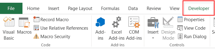
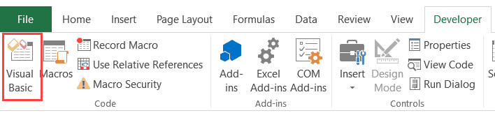
Go to the Developer tab.
Click on the Visual Basic option. This will open the VB editor in the backend.
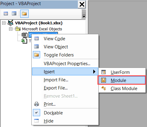
In the Project Explorer pane in the VB Editor, right-click on any object for the workbook in which you want to insert the code. If you don’t see the Project Explorer, go to the View tab and click on Project Explorer.
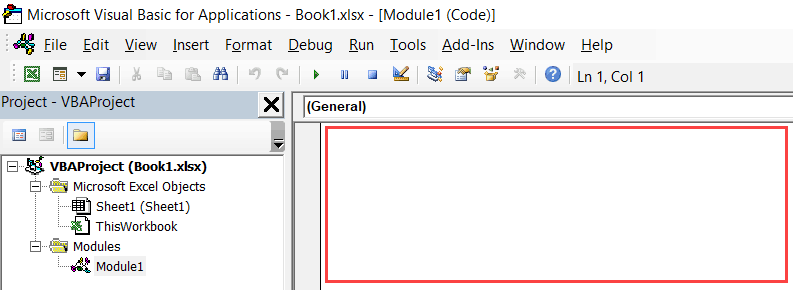
Go to Insert and click on Module. This will insert a module object for your workbook.
Copy and paste the code in the module window.

You May Also Like the Following Excel Tutorials:

Working with Worksheets using VBA.
Working with Workbooks using VBA.
Creating User-Defined Functions in Excel.
For Next Loop in Excel VBA – A Beginner’s Guide with Examples.
How to Use Excel VBA InStr Function (with practical EXAMPLES).
Excel VBA Msgbox.
How to Record a Macro in Excel.
How to Run a Macro in Excel.
How to Create an Add-in in Excel.
Excel Personal Macro Workbook | Save & Use Macros in All Workbooks.
Excel VBA Events – An Easy (and Complete) Guide.
Excel VBA Error Handling.
How to Sort Data in Excel using VBA (A Step-by-Step Guide).
24 Useful Excel Macro Examples for VBA Beginners (Ready-to-use).

Источник

Определение адреса выделенного диапазона ячеек на листе Excel с помощью кода VBA. Определение номера первой и последней строки. Программное выделение диапазона.

Адрес выделенного диапазона

Для определения адреса выделенного диапазона ячеек в VBA Excel используется свойство Address объекта Selection.

Объект Selection — это совокупность всех выделенных ячеек на листе Excel. Это может быть одна ячейка, смежный или несмежный диапазон ячеек, представляющий коллекцию смежных диапазонов. Если выделение состоит из несмежного диапазона, адреса смежных диапазонов, из которых он состоит, будут перечислены через запятую.

Смежный диапазон — прямоугольная область смежных (прилегающих друг к другу) ячеек.

Несмежный диапазон — совокупность (коллекция) смежных диапазонов (прямоугольных областей смежных ячеек).

Стоит отметить: несмотря на то, что в выделенном диапазоне может содержаться много ячеек, активной может быть только одна. Она представлена объектом ActiveCell. Для определения ее адреса в коде VBA Excel также используется свойство Address.

Sub Primer1()

MsgBox «Адрес выделенного диапазона: « & Selection.Address & _

vbNewLine & «Адрес активной ячейки: « & ActiveCell.Address & _

vbNewLine & «Номер строки активной ячейки: « & ActiveCell.Row & _

vbNewLine & «Номер столбца активной ячейки: « & ActiveCell.Column

End Sub

Скопируйте и запустите код на выполнение. В результате получите что-то вроде этого, зависящее от того, какие диапазоны вы выберите:

Определение адресов выделенного диапазона и активной ячейки

Выделение ячеек и диапазонов

Выделить несмежный диапазон ячеек можно следующим образом:

Sub Primer2()

Range(«B4:C7,E5:F7,D8»).Select

End Sub

Как видно из примера, в адресной строке объекта Range перечисляются адреса смежных диапазонов, составляющих общий несмежный диапазон, через запятую. Выделение осуществляется методом Select объекта Range.

Определение номеров первой и последней строки

Чтобы вычислить номера первой и последней строки выделенного диапазона, будем исходить из того, что первая ячейка смежного диапазона находится на первой строке, а последняя — на последней строке выделенного диапазона.

Sub Primer3()

Dim i1 As Long, i2 As Long

i1 = Selection.Cells(1).Row

i2 = Selection.Cells(Selection.Cells.Count).Row

MsgBox «Первая строка: « & i1 & _

vbNewLine & «Последняя строка: « & i2

End Sub

Результат будет таким, зависит от выделенного диапазона:

Номера первой и последней строки выделенного смежного диапазона

Таким же образом можно вычислить номера первого и последнего столбцов выделенного диапазона, которые можно использовать для обработки информации по столбцам.

Обратите внимание, что для несмежных диапазонов этот пример не работает.

На практике я использовал определение номеров первой и последней строк по выделенному диапазону для формирования файла загрузки данных держателей дисконтных карт на сервис отправки СМС-сообщений. Оказалось, что базу данных клиентов заполнять в таблице Excel намного удобнее, чем на портале сервиса, а для загрузки в сервис достаточно сформировать несложный файл. Заполнил новые строки, выделил их по любому столбцу, нажал кнопку и файл готов.

Источник

A1: Name	B1: Sales	C1: Quantity
A2: a	B2: $10	C2: 5
A3: b	B3:	C3: 10
A4: c	B4: $10	C4: 5
A5:	B5:	C5:
A6: Total	B6: $20	C6: 20