Vba excel if isna - Word и Excel - помощь в работе с программами

Date yes Add (Subtract) Days to a Date Concatenate Dates Convert Date to Number Convert Date to Text Month Name to Number Create Date Range from Dates Day Number of Year Month Name from Date First Day of Month Add (Subtract) Weeks to a Date If Functions with Dates Max Date Number of Days Between Dates Number of Days in a Month Number of Weeks Between Dates Number of Years Between Dates Split Date & Time into Separate Cells Countdown Remaining Days Insert Dates Random Date Generator Using Dynamic Ranges — Year to Date Values Add (Subtract) Years to a Date Date Formula Examples Extract Day from Date Get Day Name from Date Count Days Left in Month / Year Count Workdays Left in Month / Year Get Last Day of Month Last Business Day of Month / Year Number of Work / Business Days in Month Weekday Abbreviations Auto Populate Dates Number of Months Between Dates Quarter from a Date Years of Service Change Date Format Compare Dates Time yes Add (Subtract) Hours to Time Add (Subtract) Minutes to Time Add (Subtract) Seconds to Time Add Up time (Total Time) Time Differences Change Time Format Convert Minutes to Hours Convert Time to Decimal Convert Time to Hours Convert Time to Minutes Convert Time to Seconds Military Time Round Time to Nearest 15 Minutes Overtime Calculator Number of Hours Between Times Convert Seconds to Minutes, Hours, or Time Count Hours Worked Time Differences Time Format — Show Minutes Seconds Text yes Add Commas to Cells Get First Word from Text Capitalize First Letter Clean & Format Phone #s Remove Extra Trailing / Leading Spaces Add Spaces to Cell Assign Number Value to Text Combine Cells with Comma Combine First and Last Names Convert Text String to Date Convert Text to Number Extract Text From Cell Get Last Word Remove Unwated Characters Extract Text Before or After Character How to Split Text String by Space, Comma, & More Remove Special Characters Remove First Characters from Left Substitute Multiple Values Switch First & Last Names w/ Commas Remove Specific Text from a Cell Extract Text Between Characters (Ex. Parenthesis) Add Leading Zeros to a Number Remove Line Breaks from Text Remove all Numbers from Text Reverse Text Remove Non-Numeric Characters Remove Last Character(s) From Right Separate First and Last Names Separate Text & Numbers Round yes Round Formulas Round Price to Nearest Dollar or Cent Round to Nearest 10, 100, or 1000 Round to Nearest 5 or .5 Round Percentages Round to Significant Figures Count yes Count Blank and Non-blank Cells Count Cells Between Two Numbers Count Cells not Equal to Count if Cells are in Range Count Times Word Appears in Cell Count Words in Cell Count Specific Characters in Column Count Total Number of Characters in Column Count Cells that Equal one of two Results Count Cells that do not Contain Count Cells that Contain Specific Text Count Unique Values in Range Countif — Multiple Criteria Count Total Number of Cells in Range Count Cells with Any Text Count Total Cells in a Table Lookup yes Two Dimensional VLOOKUP VLOOKUP Simple Example Vlookup — Multiple Matches Case Sensitive Lookup Case Sensitive VLOOKUP Sum if — VLOOKUP Case Sensitive Lookup Case Sensitive VLOOKUP Find Duplicates w/ VLOOKUP or MATCH INDEX MATCH MATCH Lookup — Return Cell Address (Not Value) Lookup Last Value in Column or Row Reverse VLOOKUP (Right to Left) Risk Score Bucket with VLOOKUP Sum with a VLOOKUP Function VLOOKUP & INDIRECT VLOOKUP Concatenate VLOOKUP Contains (Partial Match) 17 Reasons Why Your XLOOKUP is Not Working Double (Nested) XLOOKUP — Dynamic Columns IFERROR (& IFNA) XLOOKUP Lookup Min / Max Value Nested VLOOKUP Top 11 Alternatives to VLOOKUP (Updated 2022!) VLOOKUP – Dynamic Column Reference VLOOKUP – Fix #N/A Error VLOOKUP – Multiple Sheets at Once VLOOKUP & HLOOKUP Combined VLOOKUP & MATCH Combined VLOOKUP Between Worksheets or Spreadsheets VLOOKUP Duplicate Values VLOOKUP Letter Grades VLOOKUP Return Multiple Columns VLOOKUP Returns 0? Return Blank Instead VLOOKUP w/o #N/A Error XLOOKUP Multiple Sheets at Once XLOOKUP Between Worksheets or Spreadsheets XLOOKUP by Date XLOOKUP Duplicate Values XLOOKUP Multiple Criteria XLOOKUP Return Multiple Columns XLOOKUP Returns 0? Return Blank Instead XLOOKUP Text XLOOKUP with IF XLOOKUP With If Statement Misc. yes Sort Multiple Columns Use Cell Value in Formula Percentage Change Between Numbers Percentage Breakdown Rank Values Add Spaces to Cell CAGR Formula Average Time Decimal Part of Number Integer Part of a Number Compare Items in a List Dealing with NA() Errors Get Worksheet Name Wildcard Characters Hyperlink to Current Folder Compound Interest Formula Percentage Increase Create Random Groups Sort with the Small and Large Functions Non-volatile Function Alternatives Decrease a Number by a Percentage Calculate Percent Variance Profit Margin Calculator Convert Column Number to Letter Get Full Address of Named Range Insert File Name Insert Path Latitute / Longitude Functions Replace Negative Values Reverse List Range Convert State Name to Abbreviation Create Dynamic Hyperlinks Custom Sort List with Formula Data Validation — Custom Formulas Dynamic Sheet Reference (INDIRECT) Reference Cell in Another Sheet or Workbook Get Cell Value by Address Get Worksheet Name Increment Cell Reference List Sheet Names List Skipped Numbers in Sequence Return Address of Max Value in Range Search by Keywords Select Every Other (or Every nth) Row Basics yes Cell Reference Basics — A1, R1C1, 3d, etc. Add Up (Sum) Entire Column or Row Into to Dynamic Array Formulas Conversions yes Convert Time Zones Convert Celsius to Fahrenheit Convert Pounds to Kilograms Convert Time to Unix Time Convert Feet to Meters Convert Centimeters to Inches Convert Kilometers to Miles Convert Inches to Feet Convert Date to Julian Format Convert Column Letter to Number Tests yes Test if a Range Contains any Text Test if any Cell in Range is Number Test if a Cell Contains a Specific Value Test if Cell Contains Any Number Test if Cell Contains Specific Number Test if Cell is Number or Text If yes Percentile If Subtotal If Sumproduct If Large If and Small If Median If Concatentate If Max If Rank If TEXTJOIN If Sum yes Sum if — Begins With / Ends With Sum if — Month or Year to Date Sum if — By Year Sum if — Blank / Non-Blank Sum if — Horizontal Sum Count / Sum If — Cell Color INDIRECT Sum Sum If — Across Multiple Sheets Sum If — By Month Sum If — Cells Not Equal To Sum If — Not Blank Sum if — Between Values Sum If — Week Number Sum Text Sum if — By Category or Group Sum if — Cell Contains Specific Text (Wildcards) Sum if — Date Rnage Sum if — Dates Equal Sum if — Day of Week Sum if — Greater Than Sum if — Less Than Average yes Average Non-Zero Values Average If — Not Blank Average — Ignore 0 Average — Ignore Errors Math yes Multiplication Table Cube Roots nth Roots Square Numbers Square Roots Calculations yes Calculate a Ratio Calculate Age KILLLLLLL Calculate Loan Payments GPA Formula Calculate VAT Tax How to Grade Formulas Find yes Find a Number in a Column / Workbook Find Most Frequent Numbers Find Smallest n Values Find nth Occurance of Character in Text Find and Extract Number from String Find Earliest or Latest Date Based on Criteria Find First Cell with Any Value Find Last Row Find Last Row with Data Find Missing Values Find Largest n Values Most Frequent Number Conditional Formatting yes Conditional Format — Dates & Times Conditional Format — Highlight Blank Cells New Functions XLOOKUP Replaces VLOOKUP, HLOOKUP, and INDEX / MATCH Logical yes AND Checks whether all conditions are met. TRUE/FALSE IF If condition is met, do something, if not, do something else. IFERROR If result is an error then do something else. NOT Changes TRUE to FALSE and FALSE to TRUE. OR Checks whether any conditions are met. TRUE/FALSE XOR Checks whether one and only one condition is met. TRUE/FALSE Lookup & Reference yes FALSE The logical value: FALSE. TRUE The logical value: TRUE. ADDRESS Returns a cell address as text. AREAS Returns the number of areas in a reference. CHOOSE Chooses a value from a list based on it’s position number. COLUMN Returns the column number of a cell reference. COLUMNS Returns the number of columns in an array. HLOOKUP Lookup a value in the first row and return a value. HYPERLINK Creates a clickable link. INDEX Returns a value based on it’s column and row numbers. INDIRECT Creates a cell reference from text. LOOKUP Looks up values either horizontally or vertically. MATCH Searches for a value in a list and returns its position. OFFSET Creates a reference offset from a starting point. ROW Returns the row number of a cell reference. ROWS Returns the number of rows in an array. TRANSPOSE Flips the oriention of a range of cells. VLOOKUP Lookup a value in the first column and return a value. Date & Time yes DATE Returns a date from year, month, and day. DATEDIF Number of days, months or years between two dates. DATEVALUE Converts a date stored as text into a valid date DAY Returns the day as a number (1-31). DAYS Returns the number of days between two dates. DAYS360 Returns days between 2 dates in a 360 day year. EDATE Returns a date, n months away from a start date. EOMONTH Returns the last day of the month, n months away date. HOUR Returns the hour as a number (0-23). MINUTE Returns the minute as a number (0-59). MONTH Returns the month as a number (1-12). NETWORKDAYS Number of working days between 2 dates. NETWORKDAYS.INTL Working days between 2 dates, custom weekends. NOW Returns the current date and time. SECOND Returns the second as a number (0-59) TIME Returns the time from a hour, minute, and second. TIMEVALUE Converts a time stored as text into a valid time. TODAY Returns the current date. WEEKDAY Returns the day of the week as a number (1-7). WEEKNUM Returns the week number in a year (1-52). WORKDAY The date n working days from a date. WORKDAY.INTL The date n working days from a date, custom weekends. YEAR Returns the year. YEARFRAC Returns the fraction of a year between 2 dates. Engineering yes CONVERT Convert number from one unit to another. Financial yes FV Calculates the future value. PV Calculates the present value. NPER Calculates the total number of payment periods. PMT Calculates the payment amount. RATE Calculates the interest Rate. NPV Calculates the net present value. IRR The internal rate of return for a set of periodic CFs. XIRR The internal rate of return for a set of non-periodic CFs. PRICE Calculates the price of a bond. YIELD Calculates the bond yield. INTRATE The interest rate of a fully invested security. Information yes CELL Returns information about a cell. ERROR.TYPE Returns a value representing the cell error. ISBLANK Test if cell is blank. TRUE/FALSE ISERR Test if cell value is an error, ignores #N/A. TRUE/FALSE ISERROR Test if cell value is an error. TRUE/FALSE ISEVEN Test if cell value is even. TRUE/FALSE ISFORMULA Test if cell is a formula. TRUE/FALSE ISLOGICAL Test if cell is logical (TRUE or FALSE). TRUE/FALSE ISNA Test if cell value is #N/A. TRUE/FALSE ISNONTEXT Test if cell is not text (blank cells are not text). TRUE/FALSE ISNUMBER Test if cell is a number. TRUE/FALSE ISODD Test if cell value is odd. TRUE/FALSE ISREF Test if cell value is a reference. TRUE/FALSE ISTEXT Test if cell is text. TRUE/FALSE N Converts a value to a number. NA Returns the error: #N/A. TYPE Returns the type of value in a cell. Math yes ABS Calculates the absolute value of a number. AGGREGATE Define and perform calculations for a database or a list. CEILING Rounds a number up, to the nearest specified multiple. COS Returns the cosine of an angle. DEGREES Converts radians to degrees. DSUM Sums database records that meet certain criteria. EVEN Rounds to the nearest even integer. EXP Calculates the exponential value for a given number. FACT Returns the factorial. FLOOR Rounds a number down, to the nearest specified multiple. GCD Returns the greatest common divisor. INT Rounds a number down to the nearest integer. LCM Returns the least common multiple. LN Returns the natural logarithm of a number. LOG Returns the logarithm of a number to a specified base. LOG10 Returns the base-10 logarithm of a number. MOD Returns the remainder after dividing. MROUND Rounds a number to a specified multiple. ODD Rounds to the nearest odd integer. PI The value of PI. POWER Calculates a number raised to a power. PRODUCT Multiplies an array of numbers. QUOTIENT Returns the integer result of division. RADIANS Converts an angle into radians. RAND Calculates a random number between 0 and 1. RANDBETWEEN Calculates a random number between two numbers. ROUND Rounds a number to a specified number of digits. ROUNDDOWN Rounds a number down (towards zero). ROUNDUP Rounds a number up (away from zero). SIGN Returns the sign of a number. SIN Returns the sine of an angle. SQRT Calculates the square root of a number. SUBTOTAL Returns a summary statistic for a series of data. SUM Adds numbers together. SUMIF Sums numbers that meet a criteria. SUMIFS Sums numbers that meet multiple criteria. SUMPRODUCT Multiplies arrays of numbers and sums the resultant array. TAN Returns the tangent of an angle. TRUNC Truncates a number to a specific number of digits. Stats yes AVERAGE Averages numbers. AVERAGEA Averages numbers. Includes text & FALSE =0, TRUE =1. AVERAGEIF Averages numbers that meet a criteria. AVERAGEIFS Averages numbers that meet multiple criteria. CORREL Calculates the correlation of two series. COUNT Counts cells that contain a number. COUNTA Count cells that are non-blank. COUNTBLANK Counts cells that are blank. COUNTIF Counts cells that meet a criteria. COUNTIFS Counts cells that meet multiple criteria. FORECAST Predict future y-values from linear trend line. FREQUENCY Counts values that fall within specified ranges. GROWTH Calculates Y values based on exponential growth. INTERCEPT Calculates the Y intercept for a best-fit line. LARGE Returns the kth largest value. LINEST Returns statistics about a trendline. MAX Returns the largest number. MEDIAN Returns the median number. MIN Returns the smallest number. MODE Returns the most common number. PERCENTILE Returns the kth percentile. PERCENTILE.INC Returns the kth percentile. Where k is inclusive. PERCENTILE.EXC Returns the kth percentile. Where k is exclusive. QUARTILE Returns the specified quartile value. QUARTILE.INC Returns the specified quartile value. Inclusive. QUARTILE.EXC Returns the specified quartile value. Exclusive. RANK Rank of a number within a series. RANK.AVG Rank of a number within a series. Averages. RANK.EQ Rank of a number within a series. Top Rank. SLOPE Calculates the slope from linear regression. SMALL Returns the kth smallest value. STDEV Calculates the standard deviation. STDEV.P Calculates the SD of an entire population. STDEV.S Calculates the SD of a sample. STDEVP Calculates the SD of an entire population TREND Calculates Y values based on a trendline. Text yes CHAR Returns a character specified by a code. CLEAN Removes all non-printable characters. CODE Returns the numeric code for a character. CONCATENATE Combines text together. DOLLAR Converts a number to text in currency format. EXACT Test if cells are exactly equal. Case-sensitive. TRUE/FALSE FIND Locates position of text within a cell.Case-sensitive. LEFT Truncates text a number of characters from the left. LEN Counts number of characters in text. LOWER Converts text to lower case. MID Extracts text from the middle of a cell. PROPER Converts text to proper case. REPLACE Replaces text based on it’s location. REPT Repeats text a number of times. RIGHT Truncates text a number of characters from the right. SEARCH Locates position of text within a cell.Not Case-sensitive. SUBSTITUTE Finds and replaces text. Case-sensitive. TEXT Converts a value into text with a specific number format. TRIM Removes all extra spaces from text. UPPER Converts text to upper case. VALUE Converts a number stored as text into a number.

Источник

Содержание

Метод WorksheetFunction.IsNA (Excel)
Синтаксис
Параметры
Возвращаемое значение
Примечания
Поддержка и обратная связь
ISNA – Test if cell is #N/A – Excel, VBA, & Google Sheets
ISNA Function Overview
ISNA Function Syntax and Inputs:
How to use the ISNA Function
ISERROR, ISERR, and ISNA
IFNA Function
Other Logical Functions
ISNA in Google Sheets
ISNA Examples in VBA
If ISNA & IFNA in VLOOKUPs – Excel & Google Sheets
IFNA in VLOOKUP
IF ISNA in VLOOKUP
IFERROR – VLOOKUP
If ISNA & IFNA in VLOOKUPs – Google Sheets
Check Excel #N/A using ISNA Function
Cause of Excel #N/A
Check Excel #N/A using worksheet formula
Check Excel #N/A using VBA
Method 1
Method 2
Method 3
How to Use IF ISNA to Hide VLOOKUP Errors
The ISNA Formula
The IF ISNA Formula Combination
Using IF ISNA with VLOOKUP
What Excel Does
Conclusion
12 thoughts on “How to Use IF ISNA to Hide VLOOKUP Errors”

Метод WorksheetFunction.IsNA (Excel)

Проверяет тип значения и возвращает значение True или False в зависимости от того, ссылается ли значение на значение ошибки #N/A (значение недоступно).

Синтаксис

expression. IsNA (Arg1)

Выражение Переменная, представляющая объект WorksheetFunction .

Параметры

Имя	Обязательный или необязательный	Тип данных	Описание
Arg1	Обязательный	Variant	Value — значение, которое требуется протестировать. Значение может быть пустым (пустая ячейка), ошибкой, логическим, текстовым, числом или ссылочным значением или именем, ссылающимся на любое из этих значений, которое требуется проверить.

Возвращаемое значение

Boolean

Примечания

Аргументы значений функций IS не преобразуются. Например, в большинстве других функций, где требуется число, текстовое значение 19 преобразуется в число 19. Однако в формуле ISNUMBER(«19») значение 19 не преобразуется из текстового значения, и функция IsNumber возвращает значение False.

Функции IS полезны в формулах для проверки результата вычисления. В сочетании с функцией IF они предоставляют метод для обнаружения ошибок в формулах.

Поддержка и обратная связь

Есть вопросы или отзывы, касающиеся Office VBA или этой статьи? Руководство по другим способам получения поддержки и отправки отзывов см. в статье Поддержка Office VBA и обратная связь.

Источник

ISNA – Test if cell is #N/A – Excel, VBA, & Google Sheets

Download the example workbook

This tutorial demonstrates how to use the Excel ISNA Function in Excel to test if a cell results in #N/A.

ISNA Function Overview

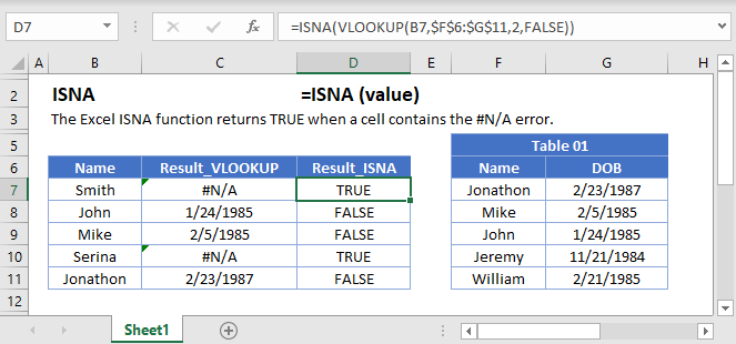
The ISNA Function Test if cell value is #N/A. Returns TRUE or FALSE.

To use the ISNA Excel Worksheet Function, select a cell and type:

(Notice how the formula inputs appear)

ISNA Function Syntax and Inputs:

value – The test value

How to use the ISNA Function

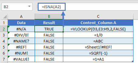
The ISNA Function checks if a calculation results in any error, except the #N/A error.

ISERROR, ISERR, and ISNA

There are two other error checking “is” functions:

The ISERROR Function returns TRUE for all errors.
The ISERR Function returns TRUE for all errors except #N/A errors.

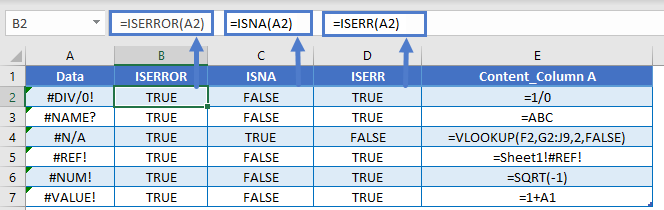
The different “is error” functions exist so you can decide what to do about potentially valid #N/A errors.

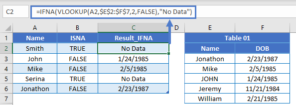
IFNA Function

Instead of the ISNA Function, you can also use the IFNA Function to do something if an error is detected (instead of simply returning TRUE / FALSE).

Other Logical Functions

Excel / Google Sheets contain many other logical functions to perform other logical tests. Here is a list:

IF / IS Functions
iferror
iserror
isna
iserr
isblank
isnumber
istext
isnontext
isformula
islogical
isref
iseven
isodd

ISNA in Google Sheets

The ISNA Function works exactly the same in Google Sheets as in Excel:

ISNA Examples in VBA

You can also use the ISNA function in VBA. Type:

On the sheet below

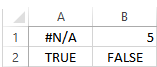
Executing the following VBA code

will return TRUE for cell A1, which is #N/A, and false for cell B2 which is 5

For the function arguments (value, etc.), you can either enter them directly into the function, or define variables to use instead.

Источник

If ISNA & IFNA in VLOOKUPs – Excel & Google Sheets

This tutorial will demonstrate how to handle VLOOKUP #N/A errors in Excel and Google Sheets. If you have access to the XLOOKUP Function, read our article on handling XLOOKUP errors.

IFNA in VLOOKUP

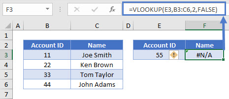
When you lookup a value with the VLOOKUP Function, if the value is not found, VLOOKUP will return the #N/A error.

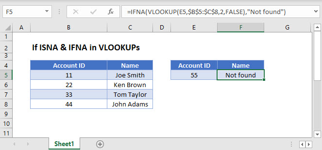
You can add the IFNA Function outside of the VLOOKUP, to do something else if the VLOOKUP results in an IFNA error. In this example, we will output “Not found” if the VLOOKUP results in an #N/A error:

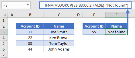
Note: The new XLOOKUP Function has built-in error handling. The IFNA Function is not needed!

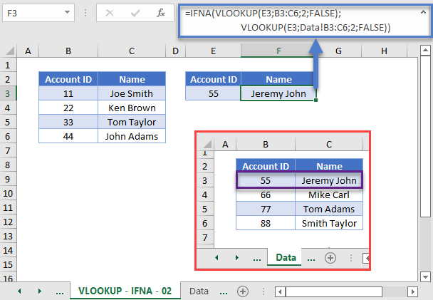
Another common use of the IFNA Function is to perform a second VLOOKUP if the first VLOOKUP can not find the value. This may be used if a value could be found on one of two sheets; if the value is not found on the first sheet, lookup the value on the second sheet instead.

IF ISNA in VLOOKUP

The IFNA Function was introduced in Excel 2013. Prior to that, you had to use the more complicated IF / ISNA combination:

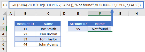
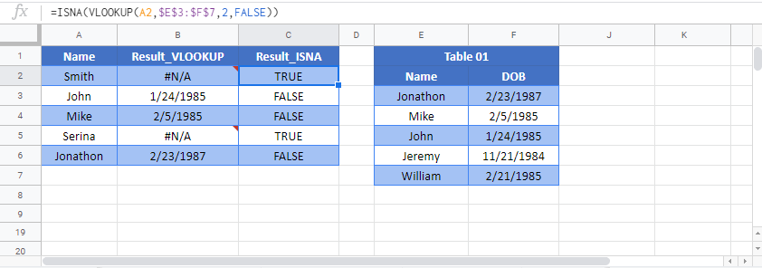
The ISNA function checks whether the result of the VLOOKUP formula is an #N/A error and returns True or False accordingly. If it is true (i.e., your lookup value is missing from the lookup array), the IF function will return with a message you specify, otherwise it will give you the result of the VLOOKUP.

IFERROR – VLOOKUP

As stated above, the IFNA Function tests if the formula outputs only a #N/A error. Instead, the IFERROR Function can be used to check if ANY error is returned:

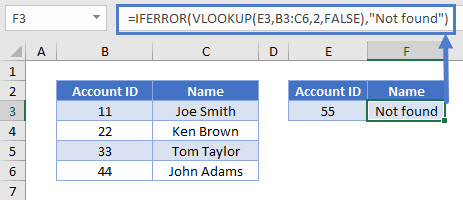
Usually it’s better to use IFNA instead of IFERROR, as IFERROR will handle errors that might need your attention.

If ISNA & IFNA in VLOOKUPs – Google Sheets

These formulas work the same in Google Sheets as in Excel.

Источник

Check Excel #N/A using ISNA Function

This Excel tutorial explains how to check Excel #N/A cells using worksheet formula ISNA and VBA Function.

You may also want to read:

Cause of Excel #N/A

#N/A is usually caused by lookup related functions where a value cannot be found in lookup table. Lookup Functions include Vlookup, Match, HLookup, Lookup.

Another common cause is that when you use an Add-In formula, and then send the file to someone who doesn’t have that Add-In. The formula was fine at the time of open the workbook but the formula will turn #N/A once formula is triggered to recalculate.

Check Excel #N/A using worksheet formula

If you want to prevent #N/A in a template with Vlookup formula, you can use IFERROR Function, which captures #N/A as well as other errors. For example

If you try to check if the Cell contains exactly #N/A, use ISNA Function. For example, if A2 contains #N/A then

Check Excel #N/A using VBA

Excel #N/A is extremely annoying in VBA because it probably causes all the subsequent VBA code to fail.

Method 1

To capture Excel #N/A in VBA, the best way is to use the worksheet function ISNA.

Method 2

Alternatively, you can also use Range.Text

Range.Text is what the screen displays, do not use Range.Value because it gets the underlying value.

Method 3

Finally, you can also use On Error Resume Next to skip the error.

Источник

How to Use IF ISNA to Hide VLOOKUP Errors

When writing a series of VLOOKUP formulas, one of the annoying things is having to see the “#N/A” error after Excel has determined a lookup value is not available. While we don’t want to show any values when they are truly unavailable, from a visual design perspective, it’s sometimes better just to show a blank space or a “not found” message. Doing so makes the output look more polished and visually appealing. It also draws less attention to the error values and lets you focus on the values that you have actually found.

The best way to mask “#N/A” errors is by using the IF ISNA formula combination. It’s important to note that you can also use IFERROR to perform the same task, and using IFERROR does require fewer inputs. However, IFERROR is prone to causing errors because it will mask all error types, including the ones that are not “#N/A” errors. Therefore, using IF ISNA is what I recommend.

The ISNA Formula

= ISNA ( value )

The ISNA formula by itself is very simple. All it does is return a “TRUE” or “FALSE” value based on whether or not an input value is equivalent to the “#N/A” error.

For example, if I were to write the ISNA formal to reference one of the “#N/A” values from our previous table, it would return with a “TRUE” result. If I were to write the same formula for another cell, that didn’t have the “#N/A” error, the result would be “FALSE”.

The IF ISNA Formula Combination

= IF ( ISNA ( original formula ) , value_if_error , original formula )

To use the IF ISNA formula combination, you just need to wrap the ISNA formula inside an IF logic condition.

The key to using the IF ISNA formula combination is that you need to put in your original formula twice

Writing your formula twice makes the process take a bit longer, but it is a necessary step to get the formula to work. Below we’ll go through an example with VLOOKUP.

Using IF ISNA with VLOOKUP

Objective : To write a VLOOKUP formula returning multiple values while masking the “#N/A” error whenever it comes up

Step 1 : Start your IF Statement

Step 2 : Start your ISNA Statement

Step 3 : Write your original intended formula

In this case it is a basic VLOOKUP formula. Click here for a tutorial on VLOOKUP.

Step 4 : Close out your ISNA Statement

This is important because you need to add another parenthesis after you’ve finished your VLOOKUP formula. This is a very easy part to miss because your VLOOKUP also ends in a parenthesis. After putting in the parenthesis, close out the logical_test with a comma.

Step 5 : Enter your error condition

The error condition is what we want to show up in place of the “#N/A” error, or the value_if_true within the IF Statement. For this example we’ll use a ” – ” to indicate the value is not available, as for this particular exercise, we’ll essentially assume countries that do not show up in the source data have a value of 0.

Step 6 : Re-enter your original formula (which is your non-error condition)

The easiest way to do this is to copy and paste your original formula over into the last portion of the syntax. Be careful about the number of parentheses you include.

Step 7 : Close out your IF Statement

Finish your IF Statement with a final parenthesis.

Step 8 : Copy your completed formula down

Make sure that you’ve reference locked properly within the VLOOKUP formula. Once that has been confirmed, all you need to do is double click the lower right hand corner of the cell you want to copy down. This final view gives you a picture of what your data set looks like with all of the “#N/A” errors masked.

What Excel Does

The logic for Excel is really simple here. If your VLOOKUP formula returns a “#N/A” error, Excel will show whatever value you input for your error condition. If your VLOOKUP formula does not return a “#N/A” error, then Excel will show whatever value your VLOOKUP was originally intending to return. It’s important to note that Excel looks ONLY for the “#N/A” error, not any other errors that might come up.

Additionally, it should also be noted that this whole process of masking errors also works exactly same with the INDEX MATCH formula as well.

Conclusion

Using IF ISNA to mask errors is a popular trick to improve the visual output of your VLOOKUP summaries. When writing the IF ISNA formula combination, remember that you’ll need to write your original formula twice. You also need to be careful about the number of parentheses you include when writing the formula, as making a mistake here is very easy. (Sometimes Excel will catch parentheses mistakes for you, but sometimes it won’t) Overall, while it does take a bit more time to write than just using the formula itself, doing so is generally worth it if you’re using those outputs for an important meeting or deliverable.

12 thoughts on “How to Use IF ISNA to Hide VLOOKUP Errors”

This is really helpful. Surprising that this info came in handy few days after I was asked to help eliminate the preponderance of the “#N/A” in an excel sheet with data derived from the Vlookup formula. Thanks.

Источник

You can prepare the spreadsheet you like to check as described below and evaluate the special cells containing the IS Functions, it is easy to check them for True or False in VBA. Alternatively, you can write your own VBA function as shown below.

There are Excel functions which check cells for special values, for example:

=ISNA(C1)

(assumed that C1 is the cell to check). This will return True if the cell is #N/A, otherwise False.

If you want to show whether a range of cells (say «C1:C17«) has any cell containing #N/A or not, it might look sensible to use:

=if(ISNA(C1:C17); "There are #N/A's in one of the cells"; "")

Sadly, this is not the case, it will not work as expected. You can only evaluate a single cell.

However, you can do it indirectly using:

=if(COUNTIF(E1:E17;TRUE)>0; "There are #N/A's in one of the cells"; "")

assuming that each of the cells E1 through E17 contains the ISNA formulas for each cell to check:

=ISNA(C1)
=ISNA(C2)
...
=ISNA(C17)

You can hide column E by right-clicking on the column and selecting Hide in Excel’s context menu so the user of your spreadsheet cannot see this column. They can still be accessed and evaluated, even if they are hidden.

In VBA you can pass a range object as RANGE parameter and evaluate the values individually by using a FOR loop:

Public Function checkCells(Rg As Range) As Boolean
    Dim result As Boolean
    result = False
    For Each r In Rg
        If Application.WorksheetFunction.IsNA(r) Then
            result = True
            Exit For
        End If
    Next
    checkCells = result
End Function

This function uses the IsNA() function internally. It must be placed inside a module, and can then be used inside a spreadsheet like:

=checkCells(A1:E5)

It returns True, if any cell is #N/A, otherwise False. You must save the workbook as macro-enabled workbook (extension XLSM), and ensure that macros are not disabled.

Excel provides more functions like the above:

ISERROR(), ISERR(), ISBLANK(), ISEVEN(), ISODD(), ISLOGICAL(), 
ISNONTEXT(), ISNUMBER(), ISREF(), ISTEXT(), ISPMT()

For example, ISERR() checks for all cell errors except #N/A and is useful to detect calculation errors.

All of these functions are described in the built in help of Excel (press F1 and then enter «IS Functions» as search text for an explanation). Some of them can be used inside VBA, some can only be used as a cell macro function.

Источник

This Excel tutorial explains how to check Excel #N/A cells using worksheet formula ISNA and VBA Function.

You may also want to read:

Excel IFERROR Function

Cause of Excel #N/A

#N/A is usually caused by lookup related functions where a value cannot be found in lookup table. Lookup Functions include Vlookup, Match, HLookup, Lookup.

Check Excel #N/A using worksheet formula

If you want to prevent #N/A in a template with Vlookup formula, you can use IFERROR Function, which captures #N/A as well as other errors. For example

=IFERROR(VLOOKUP(D3,$A$3:$B$7,2,0),”Not found”)

If you try to check if the Cell contains exactly #N/A, use ISNA Function. For example, if A2 contains #N/A then

=ISNA(A2) returns TRUE

Excel #N/A is extremely annoying in VBA because it probably causes all the subsequent VBA code to fail.

Method 1

To capture Excel #N/A in VBA, the best way is to use the worksheet function ISNA.

For example

Application.Worksheetfunction.ISNA(A2)

Method 2

Alternatively, you can also use Range.Text

Range("A2").Text = "#N/A"

Range.Text is what the screen displays, do not use Range.Value because it gets the underlying value.

Method 3

Finally, you can also use On Error Resume Next to skip the error.

Outbound References

https://support.office.com/en-us/article/Start-the-Power-Pivot-in-Microsoft-Excel-add-in-a891a66d-36e3-43fc-81e8-fc4798f39ea8?ui=en-US&rs=en-US&ad=US

Источник

The ISNA Formula

= ISNA ( value )

The ISNA formula by itself is very simple. All it does is return a “TRUE” or “FALSE” value based on whether or not an input value is equivalent to the “#N/A” error.

The IF ISNA Formula Combination

= IF ( ISNA ( original formula ) , value_if_error , original formula )

To use the IF ISNA formula combination, you just need to wrap the ISNA formula inside an IF logic condition.

The key to using the IF ISNA formula combination is that you need to put in your original formula twice

Writing your formula twice makes the process take a bit longer, but it is a necessary step to get the formula to work. Below we’ll go through an example with VLOOKUP.

Using IF ISNA with VLOOKUP

Objective: To write a VLOOKUP formula returning multiple values while masking the “#N/A” error whenever it comes up

Step 1: Start your IF Statement

Step 2: Start your ISNA Statement

Step 3: Write your original intended formula

In this case it is a basic VLOOKUP formula. Click here for a tutorial on VLOOKUP.

Step 4: Close out your ISNA Statement

Step 5: Enter your error condition

Step 6: Re-enter your original formula (which is your non-error condition)

The easiest way to do this is to copy and paste your original formula over into the last portion of the syntax. Be careful about the number of parentheses you include.

Step 7: Close out your IF Statement

Finish your IF Statement with a final parenthesis.

Step 8: Copy your completed formula down

What Excel Does

Additionally, it should also be noted that this whole process of masking errors also works exactly same with the INDEX MATCH formula as well.

Conclusion

Источник