
In this Article
- Select Entire Rows or Columns
- Select Single Row
- Select Single Column
- Select Multiple Rows or Columns
- Select ActiveCell Row or Column
- Select Rows and Columns on Other Worksheets
- Is Selecting Rows and Columns Necessary?
- Methods and Properties of Rows & Columns
- Delete Entire Rows or Columns
- Insert Rows or Columns
- Copy & Paste Entire Rows or Columns
- Hide / Unhide Rows and Columns
- Group / UnGroup Rows and Columns
- Set Row Height or Column Width
- Autofit Row Height / Column Width
- Rows and Columns on Other Worksheets or Workbooks
- Get Active Row or Column
This tutorial will demonstrate how to select and work with entire rows or columns in VBA.
First we will cover how to select entire rows and columns, then we will demonstrate how to manipulate rows and columns.
Select Entire Rows or Columns
Select Single Row
You can select an entire row with the Rows Object like this:
Rows(5).SelectOr you can use EntireRow along with the Range or Cells Objects:
Range("B5").EntireRow.Selector
Cells(5,1).EntireRow.SelectYou can also use the Range Object to refer specifically to a Row:
Range("5:5").SelectSelect Single Column
Instead of the Rows Object, use the Columns Object to select columns. Here you can reference the column number 3:
Columns(3).Selector letter “C”, surrounded by quotations:
Columns("C").SelectInstead of EntireRow, use EntireColumn along with the Range or Cells Objects to select entire columns:
Range("C5").EntireColumn.Selector
Cells(5,3).EntireColumn.SelectYou can also use the Range Object to refer specifically to a column:
Range("B:B").SelectSelect Multiple Rows or Columns
Selecting multiple rows or columns works exactly the same when using EntireRow or EntireColumn:
Range("B5:D10").EntireRow.Selector
Range("B5:B10").EntireColumn.SelectHowever, when you use the Rows or Columns Objects, you must enter the row numbers or column letters in quotations:
Rows("1:3").Selector
Columns("B:C").SelectSelect ActiveCell Row or Column
To select the ActiveCell Row or Column, you can use one of these lines of code:
ActiveCell.EntireRow.Selector
ActiveCell.EntireColumn.SelectSelect Rows and Columns on Other Worksheets
In order to select Rows or Columns on other worksheets, you must first select the worksheet.
Sheets("Sheet2").Select
Rows(3).Select
The same goes for when selecting rows or columns in other workbooks.
Workbooks("Book6.xlsm").Activate
Sheets("Sheet2").Select
Rows(3).Select
Note: You must Activate the desired workbook. Unlike the Sheets Object, the Workbook Object does not have a Select Method.
VBA Coding Made Easy
Stop searching for VBA code online. Learn more about AutoMacro — A VBA Code Builder that allows beginners to code procedures from scratch with minimal coding knowledge and with many time-saving features for all users!

Learn More
Is Selecting Rows and Columns Necessary?
However, it’s (almost?) never necessary to actually select Rows or Columns. You don’t need to select a Row or Column in order to interact with them. Instead, you can apply Methods or Properties directly to the Rows or Columns. The next several sections will demonstrate different Methods and Properties that can be applied.
You can use any method listed above to refer to Rows or Columns.
Methods and Properties of Rows & Columns
Delete Entire Rows or Columns
To delete rows or columns, use the Delete Method:
Rows("1:4").Deleteor:
Columns("A:D").DeleteVBA Programming | Code Generator does work for you!
Insert Rows or Columns
Use the Insert Method to insert rows or columns:
Rows("1:4").Insertor:
Columns("A:D").InsertCopy & Paste Entire Rows or Columns
Paste Into Existing Row or Column
When copying and pasting entire rows or columns you need to decide if you want to paste over an existing row / column or if you want to insert a new row / column to paste your data.
These first examples will copy and paste over an existing row or column:
Range("1:1").Copy Range("5:5")or
Range("C:C").Copy Range("E:E")Insert & Paste
These next examples will paste into a newly inserted row or column.
This will copy row 1 and insert it into row 5, shifting the existing rows down:
Range("1:1").Copy
Range("5:5").Insert
This will copy column C and insert it into column E, shifting the existing columns to the right:
Range("C:C").Copy
Range("E:E").Insert
Hide / Unhide Rows and Columns
To hide rows or columns set their Hidden Properties to True. Use False to hide the rows or columns:
'Hide Rows
Rows("2:3").EntireRow.Hidden = True

'Unhide Rows
Rows("2:3").EntireRow.Hidden = False
or
'Hide Columns
Columns("B:C").EntireColumn.Hidden = True

'Unhide Columns
Columns("B:C").EntireColumn.Hidden = False
Group / UnGroup Rows and Columns
If you want to Group rows (or columns) use code like this:
'Group Rows
Rows("3:5").Group

'Group Columns
Columns("C:D").Group
To remove the grouping use this code:
'Ungroup Rows
Rows("3:5").Ungroup

'Ungroup Columns
Columns("C:D").Ungroup
This will expand all “grouped” outline levels:
ActiveSheet.Outline.ShowLevels RowLevels:=8, ColumnLevels:=8and this will collapse all outline levels:
ActiveSheet.Outline.ShowLevels RowLevels:=1, ColumnLevels:=1Set Row Height or Column Width
To set the column width use this line of code:
Columns("A:E").ColumnWidth = 30To set the row height use this line of code:
Rows("1:1").RowHeight = 30AutoMacro | Ultimate VBA Add-in | Click for Free Trial!
Autofit Row Height / Column Width
To Autofit a column:
Columns("A:B").AutofitTo Autofit a row:
Rows("1:2").AutofitRows and Columns on Other Worksheets or Workbooks
To interact with rows and columns on other worksheets, you must define the Sheets Object:
Sheets("Sheet2").Rows(3).InsertSimilarly, to interact with rows and columns in other workbooks, you must also define the Workbook Object:
Workbooks("book1.xlsm").Sheets("Sheet2").Rows(3).InsertGet Active Row or Column
To get the active row or column, you can use the Row and Column Properties of the ActiveCell Object.
MsgBox ActiveCell.Rowor
MsgBox ActiveCell.ColumnThis also works with the Range Object:
MsgBox Range("B3").ColumnСодержание
- VBA – Select (and work with) Entire Rows & Columns
- Select Entire Rows or Columns
- Select Single Row
- Select Single Column
- Select Multiple Rows or Columns
- Select ActiveCell Row or Column
- Select Rows and Columns on Other Worksheets
- VBA Coding Made Easy
- Is Selecting Rows and Columns Necessary?
- Methods and Properties of Rows & Columns
- Delete Entire Rows or Columns
- Insert Rows or Columns
- Copy & Paste Entire Rows or Columns
- Paste Into Existing Row or Column
- Insert & Paste
- Hide / Unhide Rows and Columns
- Group / UnGroup Rows and Columns
- Set Row Height or Column Width
- Autofit Row Height / Column Width
- Rows and Columns on Other Worksheets or Workbooks
- Get Active Row or Column
- VBA Code Examples Add-in
- Entire Rows and Columns
- Range.Rows property (Excel)
- Syntax
- Remarks
- Example
- Support and feedback
- Свойство Range.Rows (Excel)
- Синтаксис
- Замечания
- Пример
- Поддержка и обратная связь
- VBA Lesson 2-6: VBA for Excel for the Cells, Rows and Columns
VBA – Select (and work with) Entire Rows & Columns
In this Article
This tutorial will demonstrate how to select and work with entire rows or columns in VBA.
First we will cover how to select entire rows and columns, then we will demonstrate how to manipulate rows and columns.
Select Entire Rows or Columns
Select Single Row
You can select an entire row with the Rows Object like this:
Or you can use EntireRow along with the Range or Cells Objects:
You can also use the Range Object to refer specifically to a Row:
Select Single Column
Instead of the Rows Object, use the Columns Object to select columns. Here you can reference the column number 3:
or letter “C”, surrounded by quotations:
Instead of EntireRow, use EntireColumn along with the Range or Cells Objects to select entire columns:
You can also use the Range Object to refer specifically to a column:
Select Multiple Rows or Columns
Selecting multiple rows or columns works exactly the same when using EntireRow or EntireColumn:
However, when you use the Rows or Columns Objects, you must enter the row numbers or column letters in quotations:
Select ActiveCell Row or Column
To select the ActiveCell Row or Column, you can use one of these lines of code:
Select Rows and Columns on Other Worksheets
In order to select Rows or Columns on other worksheets, you must first select the worksheet.
The same goes for when selecting rows or columns in other workbooks.
Note: You must Activate the desired workbook. Unlike the Sheets Object, the Workbook Object does not have a Select Method.
VBA Coding Made Easy
Stop searching for VBA code online. Learn more about AutoMacro — A VBA Code Builder that allows beginners to code procedures from scratch with minimal coding knowledge and with many time-saving features for all users!
Is Selecting Rows and Columns Necessary?
However, it’s (almost?) never necessary to actually select Rows or Columns. You don’t need to select a Row or Column in order to interact with them. Instead, you can apply Methods or Properties directly to the Rows or Columns. The next several sections will demonstrate different Methods and Properties that can be applied.
You can use any method listed above to refer to Rows or Columns.
Methods and Properties of Rows & Columns
Delete Entire Rows or Columns
To delete rows or columns, use the Delete Method:
Insert Rows or Columns
Use the Insert Method to insert rows or columns:
Copy & Paste Entire Rows or Columns
Paste Into Existing Row or Column
When copying and pasting entire rows or columns you need to decide if you want to paste over an existing row / column or if you want to insert a new row / column to paste your data.
These first examples will copy and paste over an existing row or column:
Insert & Paste
These next examples will paste into a newly inserted row or column.
This will copy row 1 and insert it into row 5, shifting the existing rows down:
This will copy column C and insert it into column E, shifting the existing columns to the right:
Hide / Unhide Rows and Columns
To hide rows or columns set their Hidden Properties to True. Use False to hide the rows or columns:
Group / UnGroup Rows and Columns
If you want to Group rows (or columns) use code like this:
To remove the grouping use this code:
This will expand all “grouped” outline levels:
and this will collapse all outline levels:
Set Row Height or Column Width
To set the column width use this line of code:
To set the row height use this line of code:
Autofit Row Height / Column Width
To Autofit a row:
Rows and Columns on Other Worksheets or Workbooks
To interact with rows and columns on other worksheets, you must define the Sheets Object:
Similarly, to interact with rows and columns in other workbooks, you must also define the Workbook Object:
Get Active Row or Column
To get the active row or column, you can use the Row and Column Properties of the ActiveCell Object.
This also works with the Range Object:

VBA Code Examples Add-in
Easily access all of the code examples found on our site.
Simply navigate to the menu, click, and the code will be inserted directly into your module. .xlam add-in.
Источник
Entire Rows and Columns
This example teaches you how to select entire rows and columns in Excel VBA. Are you ready?
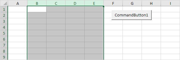
Place a command button on your worksheet and add the following code lines:
1. The following code line selects the entire sheet.
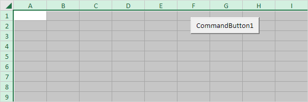
Note: because we placed our command button on the first worksheet, this code line selects the entire first sheet. To select cells on another worksheet, you have to activate this sheet first. For example, the following code lines select the entire second worksheet.
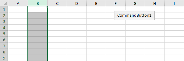
2. The following code line selects the second column.
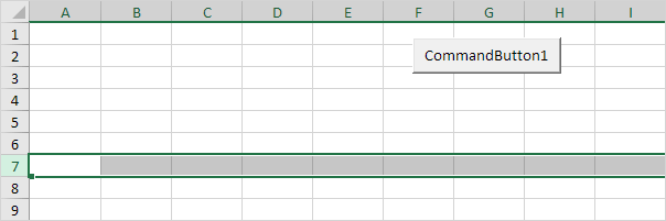
3. The following code line selects the seventh row.
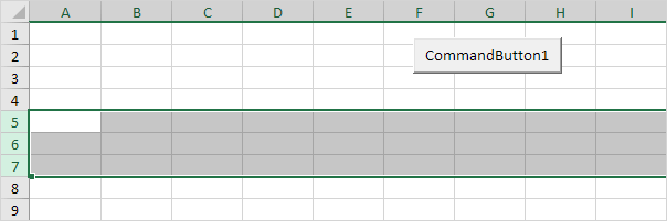
4. To select multiple rows, add a code line like this:
5. To select multiple columns, add a code line like this:
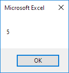
6. Be careful not to mix up the Rows and Columns properties with the Row and Column properties. The Rows and Columns properties return a Range object. The Row and Column properties return a single value.
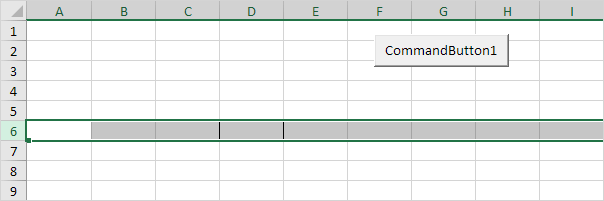
7. Select cell D6. The following code line selects the entire row of the active cell.
Note: border for illustration only.
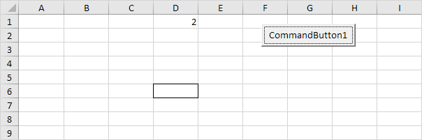
8. Select cell D6. The following code line enters the value 2 into the first cell of the column that contains the active cell.
Note: border for illustration only.
9. Select cell D6. The following code line enters the value 3 into the first cell of the row below the row that contains the active cell.
Источник
Range.Rows property (Excel)
Returns a Range object that represents the rows in the specified range.
Syntax
expression.Rows
expression A variable that represents a Range object.
To return a single row, use the Item property or equivalently include an index in parentheses. For example, both Selection.Rows(1) and Selection.Rows.Item(1) return the first row of the selection.
When applied to a Range object that is a multiple selection, this property returns rows from only the first area of the range. For example, if the Range object someRange has two areas—A1:B2 and C3:D4—, someRange.Rows.Count returns 2, not 4. To use this property on a range that may contain a multiple selection, test Areas.Count to determine whether the range is a multiple selection. If it is, loop over each area in the range, as shown in the third example.
The returned range might be outside the specified range. For example, Range(«A1:B2»).Rows(5) returns cells A5:B5. For more information, see the Item property.
Using the Rows property without an object qualifier is equivalent to using ActiveSheet.Rows. For more information, see the Worksheet.Rows property.
Example
This example deletes the range B5:Z5 on Sheet1 of the active workbook.
This example deletes rows in the current region on worksheet one of the active workbook where the value of cell one in the row is the same as the value of cell one in the previous row.
This example displays the number of rows in the selection on Sheet1. If more than one area is selected, the example loops through each area.
Support and feedback
Have questions or feedback about Office VBA or this documentation? Please see Office VBA support and feedback for guidance about the ways you can receive support and provide feedback.
Источник
Свойство Range.Rows (Excel)
Возвращает объект Range , представляющий строки в указанном диапазоне.
Синтаксис
expression. Строк
выражение: переменная, представляющая объект Range.
Замечания
Чтобы вернуть одну строку, используйте свойство Item или аналогично включите индекс в круглые скобки. Например, и Selection.Rows(1) Selection.Rows.Item(1) возвращают первую строку выделенного фрагмента.
При применении к объекту Range , который является множественным выделением, это свойство возвращает строки только из первой области диапазона. Например, если объект someRange Range имеет две области — A1:B2 и C3:D4, someRange.Rows.Count возвращает значение 2, а не 4. Чтобы использовать это свойство в диапазоне, который может содержать несколько выделенных элементов, проверьте Areas.Count , чтобы определить, является ли диапазон множественным выбором. Если это так, выполните цикл по каждой области диапазона, как показано в третьем примере.
Возвращаемый диапазон может находиться за пределами указанного диапазона. Например, Range(«A1:B2»).Rows(5) возвращает ячейки A5:B5. Дополнительные сведения см. в разделе Свойство Item .
Использование свойства Rows без квалификатора объекта эквивалентно использованию ActiveSheet.Rows. Дополнительные сведения см. в свойстве Worksheet.Rows .
Пример
В этом примере удаляется диапазон B5:Z5 на листе 1 активной книги.
В этом примере строки в текущем регионе удаляются на листе одной из активных книг, где значение ячейки в строке совпадает со значением ячейки в предыдущей строке.
В этом примере отображается количество строк в выделенном фрагменте на листе Sheet1. Если выбрано несколько областей, в примере выполняется цикл по каждой области.
Поддержка и обратная связь
Есть вопросы или отзывы, касающиеся Office VBA или этой статьи? Руководство по другим способам получения поддержки и отправки отзывов см. в статье Поддержка Office VBA и обратная связь.
Источник
VBA Lesson 2-6: VBA for Excel for the Cells, Rows and Columns
Here is some code to move around and work with the components (rows, columns, cells and their values and formulas) of a worksheet.
Selection and ActiveCell
The object Selection comprises what is selected. It can be a single cell, many cells, a column, a row,many of these, a chart, an image or any other object.
For example:
Range(«A1:A30»).Select
Selection.ClearContents
will remove the content (values or formulas) of the cells A1 to A30..
The ActiveCell is the selected cell or the first cell of the range that you have selected. Try this in Excel:
— select column A and see that cell A1 is not highlighted as the other cells. It is the ActiveCell.
— select row 3 and see that A3 is the ActiveCell.
— select cells D3 to G13 starting with D3 and see that D3 is the ActiveCell
— now select the same range but start with G13. So select G13 to D3 and see that G13 is the ActiveCell
The ActiveCell is a very important concept that you will need to remember as you start developing more complex procedures.
Delete or ClearContents
BEWARE: If you write Range(«a2»).Delete the cell A2 is destroyed and cell A3 becomes cell A2 and all the formulas that refer to cell A2 are scrapped. If you use Range(«a2»).ClearContents only the value of cell A2 is removed. In VBA Delete is a big word use it with moderation and only when you really mean Delete.
Cells and ClearContents
To select all cells you will use
Cells.Select
And the to clear them all you will write:
Selection.ClearContents
or without selecting all the cells you can still clear them all with:
Cells.ClearContents
To select a cell you will write:
Range («A1»).Select
To select a set of contiguous cells you will write:
Range («A1:A5»).Select
To select a set of non contiguous cells you will write:
Range («A1,A5,B4»).Select
Columns, Rows, Select, EntireRow, EntireColumn
To select a column you will write:
Columns(«A»).Select
To select a set of contiguous columns you will write:
Columns («A:B»).Select
To select a set of non contiguous columns you will write:
Range(«A:A,C:C,E:E»).Select
To select a row you will write:
Rows(«1»).Select
To select a set of contiguous columns you will write:
Range(«1:1,3:3,6:6»).Select
To select a set of non contiguous columns you will write:
Rows(«1:13»).Select
You can also select the column or the row with this:
ActiveCell.EntireColumn.Select
ActiveCell.EntireRow.Select
Range(«A1»).EntireColumn.Select
Range(«A1»).EntireRow.Select
If more than one cell is selected the following code will select all rows and columns covered by the selection:
Selection.EntireColumn.Select
Selection.EntireRow.Select
When you know well your way around an Excel worksheet with VBA you can transform a set of raw data into a complex report like in: «vba-example-reporting.xls«
The Offset method is the one that you will use the most. It allows you to move right, left, up and down.
For example if you want to move 3 cells to the right, you will write:
Activecell.Offset(0,3).Select
If you want to move 3 cells to the left,
Activecell.Offset(0,-3).Select
Beware though if you are in column A this line will return an error message
If you want to move three cells down:
Activecell.Offset(3,0).Select
If you want to move three cells up:
Activecell.Offset(-3,0).Select
Here is a piece of code that you will use very frequently. If you want to select one cell and three more down:
Range(Activecell,Activecell.Offset(3,0)).Select
Range(«A1» ,Range(«A1»).Offset(3,0)).Select
When you want to enter a numerical value in a cell you will write:
Range(«A1»).Select
Selection.Value = 32
Note that you don’t need to select a cell to enter a value in it, from anywhere on the sheet you can write:
Range(«A1»).Value = 32
You can even change the value of cells on another sheet with:
Sheets(«SoAndSo»).Range(«A1»).Value = 32
BEWARE: When you send a value to a cell without selecting it the cursor doesn’t move and the Activecell remains the same it doesn’t become the cell in which you have just entered a value. So if you do Activecell.Offset(1,0).Select you will not move one cell down from the cell in which you have just entered a value but from the last cell that was selected.
You can also enter the same value in many cells with:
Range(«A1:B32»).Value = 32
If you want to enter a text in a cell you need to use the double quotes like:
Range(«A1»).Value = «Peter»
If you want to enter a text within double quotes showing in a cell you need to triple the double quotes like:
Range(«A1»).Value = «»» Peter»»»
When you want to enter a formula in a cell you will write:
Range(«A1»).Select
Selection.Formula = «=C8+C9»
Note the two equal signs (=) including the one within the double quotes like if you were entering it manually.
Again you don’t need to select a cell to enter a formula in it, from anywhere on the sheet you can write:
Range(«A1»).Formula = «=C8+C9»
If you write the following:
Range(«A1:A8»).Formula = «=C8+C9»
The formula in A1 will be =C8+C9, the formula in A2 will be =C9+C10 and so on. If you want to have the exact formula =C8+C9 in all the cells, you need to write:
Range(«A1:A8»).Formula = «=$C$8+$C$9»
If you have a date in cell A1 like January, 3 2007
Range(«A2)».Value = Month(Range(«A1»).Value the value entered in A2 will be 1
Range(«A2)».Value = Day(Range(«A1»).Value the value entered in A2 will be 3
Range(«A2)».Value = Year(Range(«A1»).Value the value entered in A2 will be 2007
Month and MonthName
As you have seen above:
Month(A1) will return «3» if there is «3/12/2007» in A1
But:
MonthName(Range(«A1»).Value) will return «January» if there is «1» in A1
MonthName(Range(«A1»).Value,True) will return «Feb» if there is «2» in A1
MonthName(Month(Range(«A1»).Value)) will return «March» if there is «3/12/2007» in A1
One of the most important property when working with sets of data and databases:
Selection.CurrentRegion.Select
will select all cells from the selection to the first empty row and the first empty column. See the lesson on databases to discover the importance of CurrentRegion
Column, Row, Columns, Rows, Count
For the following lines of code notice that you need to send the result into a variable. See lesson 2-9 on variables
Источник
If the user selects multiple rows in Microsoft Excel, the selection can contain multiple areas. An area is a subselection of rows created when the user presses the Shift button while doing a multiselect. In VBA we need to handle each area independently to be able to retrieve all the selected rows.
' Example
Public Sub Test()
    Dim objSelection As Range
    Dim objSelectionArea As Range
    Dim objCell As Range
    Dim intRow As Integer

    ' Get the current selection
    Set objSelection = Application.Selection

    ' Walk through the areas
    For Each objSelectionArea In objSelection.Areas

        ' Walk through the rows
        For intRow = 1 To objSelectionArea.Rows.Count Step 1
            ' Get the row reference
            Set objCell = objSelectionArea.Rows(intRow)

            ' Get the actual row index (in the worksheet).
            ' The other row index is relative to the collection.
            intActualRow = objCell.Row

            ' Get any cell value by using the actual row index
            ' Example:
            strName = objNameRange(intActualRow, 1).value
        Next
    Next
End Sub
In the example we have not defined the variables strName and objNameRange. For your reference the variables are defined as follows:
Dim strName As String
Dim objNameRange As Range
objNameRange can be any range in your selected worksheet.
Related
- Get Column Name from Column Index in Excel
- Get Microsoft Excel

Ulf Emsoy
Ulf Emsoy has long working experience in project management, software development and supply chain management.
Back To Top
We use cookies on our website to give you the most relevant experience by remembering your preferences and repeat visits. By clicking “Accept All”, you consent to the use of ALL the cookies. However, you may visit «Cookie Settings» to provide a controlled consent.
This example teaches you how to select entire rows and columns in Excel VBA. Are you ready?
Place a command button on your worksheet and add the following code lines:
1. The following code line selects the entire sheet.
Cells.Select
Note: because we placed our command button on the first worksheet, this code line selects the entire first sheet. To select cells on another worksheet, you have to activate this sheet first. For example, the following code lines select the entire second worksheet.
Worksheets(2).Activate
Worksheets(2).Cells.Select
2. The following code line selects the second column.
Columns(2).Select
3. The following code line selects the seventh row.
Rows(7).Select
4. To select multiple rows, add a code line like this:
Rows(«5:7»).Select
5. To select multiple columns, add a code line like this:
Columns(«B:E»).Select
6. Be careful not to mix up the Rows and Columns properties with the Row and Column properties. The Rows and Columns properties return a Range object. The Row and Column properties return a single value.
Code line:
MsgBox Cells(5, 2).Row
Result:
7. Select cell D6. The following code line selects the entire row of the active cell.
ActiveCell.EntireRow.Select
Note: border for illustration only.
8. Select cell D6. The following code line enters the value 2 into the first cell of the column that contains the active cell.
ActiveCell.EntireColumn.Cells(1).Value = 2
Note: border for illustration only.
9. Select cell D6. The following code line enters the value 3 into the first cell of the row below the row that contains the active cell.
ActiveCell.EntireRow.Offset(1, 0).Cells(1).Value = 3

Note: border for illustration only.
I found a similar solution to this question in c# How to Select all the cells in a worksheet in Excel.Range object of c#?
What is the process to do this in VBA?
I select data normally by using «ctrl+shift over arrow, down arrow» to select an entire range of cells. When I run this in a macro it codes out A1:Q398247930, for example. I need it to just be
.SetRange Range("A1:whenever I run out of rows and columns")
I could easily do it myself without a macro, but I’m trying to make the entire process a macro, and this is just a piece of it.
Sub sort()
    'sort Macro
    Range("B2").Select
    ActiveWorkbook.Worksheets("Master").sort.SortFields.Clear
    ActiveWorkbook.Worksheets("Master").sort.SortFields.Add Key:=Range("B2"), _
      SortOn:=xlSortOnValues, Order:=xlAscending, DataOption:=xlSortNormal
    With ActiveWorkbook.Worksheets("Master").sort
        .SetRange Range("A1:whenever I run out of rows and columns")
        .Header = xlNo
        .MatchCase = False
        .Orientation = xlTopToBottom
        .SortMethod = xlPinYin
        .Apply
    End With
End Sub
edit:
There are other parts where I might want to use the same code but the range is say «C3:End of rows & columns». Is there a way in VBA to get the location of the last cell in the document?
asked Jul 30, 2013 at 18:50
![]()
C. TewaltC. Tewalt
2,2612 gold badges29 silver badges47 bronze badges
I believe you want to find the current region of A1 and surrounding cells — not necessarily all cells on the sheet.
If so — simply use…
Range(«A1»).CurrentRegion
answered Jul 30, 2013 at 19:17
![]()
ExcelExpertExcelExpert
3522 silver badges4 bronze badges
1
You can simply use cells.select to select all cells in the worksheet. You can get a valid address by saying Range(Cells.Address).
If you want to find the last Used Range where you have made some formatting change or entered a value into you can call ActiveSheet.UsedRange and select it from there. Hope that helps.
![]()
June7
19.5k8 gold badges24 silver badges33 bronze badges
answered Jul 30, 2013 at 19:11
![]()
chanceachancea
5,8083 gold badges28 silver badges39 bronze badges
2
you can use all cells as a object like this :
Dim x as Range
Set x = Worksheets("Sheet name").Cells
X is now a range object that contains the entire worksheet
answered Apr 15, 2015 at 11:47
![]()
you have a few options here:
- Using the UsedRange property
- find the last row and column used
- use a mimic of shift down and shift right
I personally use the Used Range and find last row and column method most of the time.
Here’s how you would do it using the UsedRange property:
Sheets("Sheet_Name").UsedRange.Select
This statement will select all used ranges in the worksheet, note that sometimes this doesn’t work very well when you delete columns and rows.
The alternative is to find the very last cell used in the worksheet
Dim rngTemp As Range
Set rngTemp = Cells.Find("*", SearchOrder:=xlByRows, SearchDirection:=xlPrevious)
If Not rngTemp Is Nothing Then
    Range(Cells(1, 1), rngTemp).Select
End If
What this code is doing:
- Find the last cell containing any value
- select cell(1,1) all the way to the last cell
![]()
answered Jul 30, 2013 at 20:32
![]()
Derek ChengDerek Cheng
5353 silver badges8 bronze badges
3
Another way to select all cells within a range, as long as the data is contiguous, is to use Range("A1", Range("A1").End(xlDown).End(xlToRight)).Select.
answered Mar 29, 2019 at 19:38
![]()
I would recommend recording a macro, like found in this post;
Excel VBA macro to filter records
But if you are looking to find the end of your data and not the end of the workbook necessary, if there are not empty cells between the beginning and end of your data, I often use something like this;
R = 1
Do While Not IsEmpty(Sheets("Sheet1").Cells(R, 1))
    R = R + 1
Loop
Range("A5:A" & R).Select 'This will give you a specific selection
You are left with R = to the number of the row after your data ends. This could be used for the column as well, and then you could use something like Cells(C , R).Select, if you made C the column representation.
![]()
answered Jul 30, 2013 at 19:25
![]()
MakeCentsMakeCents
7321 gold badge5 silver badges15 bronze badges
2
Sub SelectAllCellsInSheet(SheetName As String)
    lastCol = Sheets(SheetName).Range("a1").End(xlToRight).Column
    Lastrow = Sheets(SheetName).Cells(1, 1).End(xlDown).Row
    Sheets(SheetName).Range("A1", Sheets(SheetName).Cells(Lastrow, lastCol)).Select
End Sub
To use with ActiveSheet:
Call SelectAllCellsInSheet(ActiveSheet.Name)
answered Mar 14, 2017 at 20:57
![]()
Yehia AmerYehia Amer
5985 silver badges11 bronze badges
Here is what I used, I know it could use some perfecting, but I think it will help others…
''STYLING''

Dim sheet As Range

' Find Number of rows used
Dim Final As Variant
    Final = Range("A1").End(xlDown).Row

' Find Last Column
Dim lCol As Long
    lCol = Cells(1, Columns.Count).End(xlToLeft).Column

Set sheet = ActiveWorkbook.ActiveSheet.Range("A" & Final & "", Cells(1, lCol ))
With sheet
    .Interior.ColorIndex = 1
End With
answered Mar 16, 2019 at 4:29
![]()
I have found that the Worksheet «.UsedRange» method is superior in many instances to solve this problem.
I struggled with a truncation issue that is a normal behaviour of the «.CurrentRegion» method. Using [ Worksheets(«Sheet1»).Range(«A1»).CurrentRegion ] does not yield the results I desired when the worksheet consists of one column with blanks in the rows (and the blanks are wanted). In this case, the «.CurrentRegion» will truncate at the first record. I implemented a work around but recently found an even better one; see code below that allows copying the whole set to another sheet or to identify the actual address (or just rows and columns):
Sub mytest_GetAllUsedCells_in_Worksheet()
    Dim myRange

    Set myRange = Worksheets("Sheet1").UsedRange
    'Alternative code:  set myRange = activesheet.UsedRange

   'use msgbox or debug.print to show the address range and counts
   MsgBox myRange.Address
   MsgBox myRange.Columns.Count
   MsgBox myRange.Rows.Count

  'Copy the Range of data to another sheet
  'Note: contains all the cells with that are non-empty
   myRange.Copy (Worksheets("Sheet2").Range("A1"))
   'Note:  transfers all cells starting at "A1" location.
   '       You can transfer to another area of the 2nd sheet
   '       by using an alternate starting location like "C5".

End Sub
answered May 2, 2019 at 19:38
![]()
Maybe this might work:
Sh.Range(«A1», Sh.Range(«A» & Rows.Count).End(xlUp))
answered Oct 31, 2014 at 18:38
![]()
Refering to the very first question, I am looking into the same.
The result I get, recording a macro, is, starting by selecting cell A76:
Sub find_last_row()
    Range("A76").Select
    Range(Selection, Selection.End(xlDown)).Select
End Sub
answered Aug 7, 2015 at 12:40
![]()
| title | keywords | f1_keywords | ms.prod | api_name | ms.assetid | ms.date | ms.localizationpriority |
|---|---|---|---|---|---|---|---|
|
Range object (Excel) |
vbaxl10.chm143072 |
vbaxl10.chm143072 |
excel |
Excel.Range |
b8207778-0dcc-4570-1234-f130532cc8cd |
08/14/2019 |
high |
Range object (Excel)
Represents a cell, a row, a column, a selection of cells containing one or more contiguous blocks of cells, or a 3D range.
[!includeAdd-ins note]
Remarks
The default member of Range forwards calls without parameters to the Value property and calls with parameters to the Item member. Accordingly, someRange = someOtherRange is equivalent to someRange.Value = someOtherRange.Value, someRange(1) to someRange.Item(1) and someRange(1,1) to someRange.Item(1,1).
The following properties and methods for returning a Range object are described in the Example section:
- Range and Cells properties of the Worksheet object
- Range and Cells properties of the Range object
- Rows and Columns properties of the Worksheet object
- Rows and Columns properties of the Range object
- Offset property of the Range object
- Union method of the Application object
Example
Use Range (arg), where arg names the range, to return a Range object that represents a single cell or a range of cells. The following example places the value of cell A1 in cell A5.
Worksheets("Sheet1").Range("A5").Value = _
    Worksheets("Sheet1").Range("A1").Value
The following example fills the range A1:H8 with random numbers by setting the formula for each cell in the range. When it’s used without an object qualifier (an object to the left of the period), the Range property returns a range on the active sheet. If the active sheet isn’t a worksheet, the method fails.
Use the Activate method of the Worksheet object to activate a worksheet before you use the Range property without an explicit object qualifier.
Worksheets("Sheet1").Activate
Range("A1:H8").Formula = "=Rand()"    'Range is on the active sheet
The following example clears the contents of the range named Criteria.
[!NOTE]
If you use a text argument for the range address, you must specify the address in A1-style notation (you cannot use R1C1-style notation).
Worksheets(1).Range("Criteria").ClearContents
Use Cells on a worksheet to obtain a range consisting all single cells on the worksheet. You can access single cells via Item(row, column), where row is the row index and column is the column index.
Item can be omitted since the call is forwarded to it by the default member of Range.
The following example sets the value of cell A1 to 24 and of cell B1 to 42 on the first sheet of the active workbook.
Worksheets(1).Cells(1, 1).Value = 24
Worksheets(1).Cells.Item(1, 2).Value = 42
The following example sets the formula for cell A2.
ActiveSheet.Cells(2, 1).Formula = "=Sum(B1:B5)"
Although you can also use Range("A1") to return cell A1, there may be times when the Cells property is more convenient because you can use a variable for the row or column. The following example creates column and row headings on Sheet1. Be aware that after the worksheet has been activated, the Cells property can be used without an explicit sheet declaration (it returns a cell on the active sheet).
[!NOTE]
Although you could use Visual Basic string functions to alter A1-style references, it is easier (and better programming practice) to use theCells(1, 1)notation.
Sub SetUpTable()
Worksheets("Sheet1").Activate
For TheYear = 1 To 5
    Cells(1, TheYear + 1).Value = 1990 + TheYear
Next TheYear
For TheQuarter = 1 To 4
    Cells(TheQuarter + 1, 1).Value = "Q" & TheQuarter
Next TheQuarter
End Sub
Use_expression_.Cells, where expression is an expression that returns a Range object, to obtain a range with the same address consisting of single cells.
On such a range, you access single cells via Item(row, column), where are relative to the upper-left corner of the first area of the range.
Item can be omitted since the call is forwarded to it by the default member of Range.
The following example sets the formula for cell C5 and D5 of the first sheet of the active workbook.
Worksheets(1).Range("C5:C10").Cells(1, 1).Formula = "=Rand()"
Worksheets(1).Range("C5:C10").Cells.Item(1, 2).Formula = "=Rand()"
Use Range (cell1, cell2), where cell1 and cell2 are Range objects that specify the start and end cells, to return a Range object. The following example sets the border line style for cells A1:J10.
[!NOTE]
Be aware that the period in front of each occurrence of the Cells property is required if the result of the preceding With statement is to be applied to the Cells property. In this case, it indicates that the cells are on worksheet one (without the period, the Cells property would return cells on the active sheet).
With Worksheets(1)
    .Range(.Cells(1, 1), _
        .Cells(10, 10)).Borders.LineStyle = xlThick
End With
Use Rows on a worksheet to obtain a range consisting all rows on the worksheet. You can access single rows via Item(row), where row is the row index.
Item can be omitted since the call is forwarded to it by the default member of Range.
[!NOTE]
It’s not legal to provide the second parameter of Item for ranges consisting of rows. You first have to convert it to single cells via Cells.
The following example deletes row 5 and 10 of the first sheet of the active workbook.
Worksheets(1).Rows(10).Delete
Worksheets(1).Rows.Item(5).Delete
Use Columns on a worksheet to obtain a range consisting all columns on the worksheet. You can access single columns via Item(row) [sic], where row is the column index given as a number or as an A1-style column address.
Item can be omitted since the call is forwarded to it by the default member of Range.
[!NOTE]
It’s not legal to provide the second parameter of Item for ranges consisting of columns. You first have to convert it to single cells via Cells.
The following example deletes column «B», «C», «E», and «J» of the first sheet of the active workbook.
Worksheets(1).Columns(10).Delete
Worksheets(1).Columns.Item(5).Delete
Worksheets(1).Columns("C").Delete
Worksheets(1).Columns.Item("B").Delete
Use_expression_.Rows, where expression is an expression that returns a Range object, to obtain a range consisting of the rows in the first area of the range.
You can access single rows via Item(row), where row is the relative row index from the top of the first area of the range.
Item can be omitted since the call is forwarded to it by the default member of Range.
[!NOTE]
It’s not legal to provide the second parameter of Item for ranges consisting of rows. You first have to convert it to single cells via Cells.
The following example deletes the ranges C8:D8 and C6:D6 of the first sheet of the active workbook.
Worksheets(1).Range("C5:D10").Rows(4).Delete
Worksheets(1).Range("C5:D10").Rows.Item(2).Delete
Use_expression_.Columns, where expression is an expression that returns a Range object, to obtain a range consisting of the columns in the first area of the range.
You can access single columns via Item(row) [sic], where row is the relative column index from the left of the first area of the range given as a number or as an A1-style column address.
Item can be omitted since the call is forwarded to it by the default member of Range.
[!NOTE]
It’s not legal to provide the second parameter of Item for ranges consisting of columns. You first have to convert it to single cells via Cells.
The following example deletes the ranges L2:L10, G2:G10, F2:F10 and D2:D10 of the first sheet of the active workbook.
Worksheets(1).Range("C5:Z10").Columns(10).Delete
Worksheets(1).Range("C5:Z10").Columns.Item(5).Delete
Worksheets(1).Range("C5:Z10").Columns("D").Delete
Worksheets(1).Range("C5:Z10").Columns.Item("B").Delete
Use Offset (row, column), where row and column are the row and column offsets, to return a range at a specified offset to another range. The following example selects the cell three rows down from and one column to the right of the cell in the upper-left corner of the current selection. You cannot select a cell that is not on the active sheet, so you must first activate the worksheet.
Worksheets("Sheet1").Activate
  'Can't select unless the sheet is active
Selection.Offset(3, 1).Range("A1").Select
Use Union (range1, range2, …) to return multiple-area ranges—that is, ranges composed of two or more contiguous blocks of cells. The following example creates an object defined as the union of ranges A1:B2 and C3:D4, and then selects the defined range.
Dim r1 As Range, r2 As Range, myMultiAreaRange As Range
Worksheets("sheet1").Activate
Set r1 = Range("A1:B2")
Set r2 = Range("C3:D4")
Set myMultiAreaRange = Union(r1, r2)
myMultiAreaRange.Select
If you work with selections that contain more than one area, the Areas property is useful. It divides a multiple-area selection into individual Range objects and then returns the objects as a collection. Use the Count property on the returned collection to verify a selection that contains more than one area, as shown in the following example.
Sub NoMultiAreaSelection()
    NumberOfSelectedAreas = Selection.Areas.Count
    If NumberOfSelectedAreas > 1 Then
        MsgBox "You cannot carry out this command " & _
            "on multi-area selections"
    End If
End Sub
This example uses the AdvancedFilter method of the Range object to create a list of the unique values, and the number of times those unique values occur, in the range of column A.
Sub Create_Unique_List_Count()
    'Excel workbook, the source and target worksheets, and the source and target ranges.
    Dim wbBook As Workbook
    Dim wsSource As Worksheet
    Dim wsTarget As Worksheet
    Dim rnSource As Range
    Dim rnTarget As Range
    Dim rnUnique As Range
    'Variant to hold the unique data
    Dim vaUnique As Variant
    'Number of unique values in the data
    Dim lnCount As Long

    'Initialize the Excel objects
    Set wbBook = ThisWorkbook
    With wbBook
        Set wsSource = .Worksheets("Sheet1")
        Set wsTarget = .Worksheets("Sheet2")
    End With

    'On the source worksheet, set the range to the data stored in column A
    With wsSource
        Set rnSource = .Range(.Range("A1"), .Range("A100").End(xlDown))
    End With

    'On the target worksheet, set the range as column A.
    Set rnTarget = wsTarget.Range("A1")

    'Use AdvancedFilter to copy the data from the source to the target,
    'while filtering for duplicate values.
    rnSource.AdvancedFilter Action:=xlFilterCopy, _
                            CopyToRange:=rnTarget, _
                            Unique:=True

    'On the target worksheet, set the unique range on Column A, excluding the first cell
    '(which will contain the "List" header for the column).
    With wsTarget
        Set rnUnique = .Range(.Range("A2"), .Range("A100").End(xlUp))
    End With

    'Assign all the values of the Unique range into the Unique variant.
    vaUnique = rnUnique.Value

    'Count the number of occurrences of every unique value in the source data,
    'and list it next to its relevant value.
    For lnCount = 1 To UBound(vaUnique)
        rnUnique(lnCount, 1).Offset(0, 1).Value = _
            Application.Evaluate("COUNTIF(" & _
            rnSource.Address(External:=True) & _
            ",""" & rnUnique(lnCount, 1).Text & """)")
    Next lnCount

    'Label the column of occurrences with "Occurrences"
    With rnTarget.Offset(0, 1)
        .Value = "Occurrences"
        .Font.Bold = True
    End With

End Sub
Methods
- Activate
- AddComment
- AddCommentThreaded
- AdvancedFilter
- AllocateChanges
- ApplyNames
- ApplyOutlineStyles
- AutoComplete
- AutoFill
- AutoFilter
- AutoFit
- AutoOutline
- BorderAround
- Calculate
- CalculateRowMajorOrder
- CheckSpelling
- Clear
- ClearComments
- ClearContents
- ClearFormats
- ClearHyperlinks
- ClearNotes
- ClearOutline
- ColumnDifferences
- Consolidate
- ConvertToLinkedDataType
- Copy
- CopyFromRecordset
- CopyPicture
- CreateNames
- Cut
- DataTypeToText
- DataSeries
- Delete
- DialogBox
- Dirty
- DiscardChanges
- EditionOptions
- ExportAsFixedFormat
- FillDown
- FillLeft
- FillRight
- FillUp
- Find
- FindNext
- FindPrevious
- FlashFill
- FunctionWizard
- Group
- Insert
- InsertIndent
- Justify
- ListNames
- Merge
- NavigateArrow
- NoteText
- Parse
- PasteSpecial
- PrintOut
- PrintPreview
- RemoveDuplicates
- RemoveSubtotal
- Replace
- RowDifferences
- Run
- Select
- SetCellDataTypeFromCell
- SetPhonetic
- Show
- ShowCard
- ShowDependents
- ShowErrors
- ShowPrecedents
- Sort
- SortSpecial
- Speak
- SpecialCells
- SubscribeTo
- Subtotal
- Table
- TextToColumns
- Ungroup
- UnMerge
Properties
- AddIndent
- Address
- AddressLocal
- AllowEdit
- Application
- Areas
- Borders
- Cells
- Characters
- Column
- Columns
- ColumnWidth
- Comment
- CommentThreaded
- Count
- CountLarge
- Creator
- CurrentArray
- CurrentRegion
- Dependents
- DirectDependents
- DirectPrecedents
- DisplayFormat
- End
- EntireColumn
- EntireRow
- Errors
- Font
- FormatConditions
- Formula
- FormulaArray
- FormulaHidden
- FormulaLocal
- FormulaR1C1
- FormulaR1C1Local
- HasArray
- HasFormula
- HasRichDataType
- Height
- Hidden
- HorizontalAlignment
- Hyperlinks
- ID
- IndentLevel
- Interior
- Item
- Left
- LinkedDataTypeState
- ListHeaderRows
- ListObject
- LocationInTable
- Locked
- MDX
- MergeArea
- MergeCells
- Name
- Next
- NumberFormat
- NumberFormatLocal
- Offset
- Orientation
- OutlineLevel
- PageBreak
- Parent
- Phonetic
- Phonetics
- PivotCell
- PivotField
- PivotItem
- PivotTable
- Precedents
- PrefixCharacter
- Previous
- QueryTable
- Range
- ReadingOrder
- Resize
- Row
- RowHeight
- Rows
- ServerActions
- ShowDetail
- ShrinkToFit
- SoundNote
- SparklineGroups
- Style
- Summary
- Text
- Top
- UseStandardHeight
- UseStandardWidth
- Validation
- Value
- Value2
- VerticalAlignment
- Width
- Worksheet
- WrapText
- XPath
See also
- Excel Object Model Reference
[!includeSupport and feedback]
10
Tuesday
Jun 2014
If the user does does a selection of rows in Excel, the selection can contain multiple areas. An area is a subselection of rows created when the user presses the Shift button while doing a multiselect. In VBA we need to handle each area independently to be able to retrieve all the selected rows.
‘ Example
Public Sub Test()
Dim objSelection As Range
Dim objSelectionArea As Range
Dim objCell As Range
Dim intRow As Integer ‘ Get the current selection
Set objSelection = Application.Selection
‘ Walk through the areas
For Each objSelectionArea In objSelection.Areas
‘ Walk through the rows
For intRow = 1 To objSelectionArea.Rows.Count Step 1
‘ Get the row reference
Set objCell = objSelectionArea.Rows(intRow)
‘ Get the actual row index (in the worksheet).
‘ The other row index is relative to the collection.
intActualRow = objCell.Row
‘ Get any cell value by using the actual row index
‘ Example:
” strName = objNameRange(intActualRow, 1).value
Next
Next
End SubIn the example we have not defined the variables strName and objNameRange. For your reference the variables are defined as follows:
Dim strName As String
Dim objNameRange As Range
objNameRange can be any range in your selected worksheet.
http://www.lazerwire.com/2011/10/excel-vba-get-all-selected-rows.html
I never imagined that my first article involving VBA will be this short. And I kept myself from diving into VBA and Macros until now so that I stay basic and all my dear readers and followers get to know the basics first. But this time I had to call the real army in! So follow along.
Selecting an entire row where active cell is already very easy. For example if your active cell is C8 and you want to select whole Row 8 then simply hit Shift+Space bar and this will select the whole row where your active cell is. Similarly if you want to select the whole column of active cell, your shortcut is Ctrl+Space bar.
But one of our member who recently joined our facebook community asked few questions and one was “how to select entire rows that contain specific text”
Now this seemingly one questions have two edges:
- find cells that contain selected texts and select them
- select all rows of the cells selected in 1
Interesting and intimidating. And this very query left me no choice but to jump in VBA world. For those who don’t know about VBA it is a short for Visual Basic for Applications and in our case application is Excel. In short, Visual Basic for Excel. Visual Basic is a programming language and if you couple the power of Excel with programming, then what Excel can do is probably limited only up to your imagination. You already know how powerful Excel is. Believe me without VBA, Excel is without a heart!
Back to our task. So first we want to find all the cells that contain the specific text we want. This could result in multiple cells getting selected and then select whole rows of the selected cells.
Finding and selecting cells with specific text
This part is easy. And I have discussed how to do this in many of my articles before. But here it is again:
Step 1: Select the range if you want to search only in selected area. If you want to search whole worksheet then proceed to step 2.
Step 2: Go to Home tab > Editing tools group > click Find & Select drop down > click Find. Or simply hit Ctrl+F shortcut.
Step 3: In the find what field type the text you want to find. If it is a word then put a whole word. If you have part of the word then you can use wildcards like asterisk (*) or question marks (?).
Step 4: Hit Find all button. This will search for the criteria provided and display the results in the same Find dialogue box.
Step 5: To select all of the cells that contain the searched word. Click any result and hit Ctrl+A. This will not only select all results but also the cells that contain that search string. Click close. Notice that cells will stay selected. And this is exactly what we need for our next step
Select entire rows of all the selected (multiple) cells
Step 1: Hit shortcut Alt+F8. This will bring up macro dialogue.
Step 2: In the name field type: selectentirerow. Make sure there are no spaces. And hit Create button.
Step 3: The moment you hit create button you will enter the strange world of VBA. Yes! This is the playground of all Excel gurus. Welcome aboard. You will get an active cursor inside a window. Active cursor will be below the line that says: Sub selectentirerow()
Step 4: Simply type this:
selection.entirerow.select
Step 5: While you are still inside VB environment, hit F5 key on the keyboard. Nothing happened??? Read next step 😉
Step 6: Come back to your original Excel window where your worksheet is. And you will see that now all the rows where you had selected cells are now selected.
Give me Hi 5! You have just excelled at VBA and one of its function 🙂
Bonus Tip – Assign shortcut key to Macro
Now that you have created a macro, you can use it again and again. To do this you can hit Alt+F8 to bring macro dialogue box, select the macro and hit Run button.
But it is much easier if you assign a shortcut key to this. To do this follow these steps:
Step 1: Hit Alt+F8 to invoke Macro dialogue box. Select the macro you created (named selectentirerow) and click Options button.
Step 2: A new dialogue box will appear. In this you can assign a key that will work in combination with Ctrl key on the keyboard. Type any letter but make sure it is not already used by Excel default features. For example if you type C, it will replace your copy shortcut. So use the key which is vacant. For example Q. Click OK. Your shortcut is now Ctrl+Q
Now you can select entire rows of selected cells easily just by hitting Ctrl+Q shortcut.
“It is a capital mistake to theorize before one has data”- Sir Arthur Conan Doyle
This post covers everything you need to know about using Cells and Ranges in VBA. You can read it from start to finish as it is laid out in a logical order. If you prefer you can use the table of contents below to go to a section of your choice.
Topics covered include Offset property, reading values between cells, reading values to arrays and formatting cells.
A Quick Guide to Ranges and Cells
| Function | Takes | Returns | Example | Gives |
|---|---|---|---|---|
|
Range |
cell address | multiple cells | .Range(«A1:A4») | $A$1:$A$4 |
| Cells | row, column | one cell | .Cells(1,5) | $E$1 |
| Offset | row, column | multiple cells | Range(«A1:A2») .Offset(1,2) |
$C$2:$C$3 |
| Rows | row(s) | one or more rows | .Rows(4) .Rows(«2:4») |
$4:$4 $2:$4 |
| Columns | column(s) | one or more columns | .Columns(4) .Columns(«B:D») |
$D:$D $B:$D |
Download the Code
The Webinar
If you are a member of the VBA Vault, then click on the image below to access the webinar and the associated source code.
(Note: Website members have access to the full webinar archive.)

Introduction
This is the third post dealing with the three main elements of VBA. These three elements are the Workbooks, Worksheets and Ranges/Cells. Cells are by far the most important part of Excel. Almost everything you do in Excel starts and ends with Cells.
Generally speaking, you do three main things with Cells
- Read from a cell.
- Write to a cell.
- Change the format of a cell.
Excel has a number of methods for accessing cells such as Range, Cells and Offset.These can cause confusion as they do similar things and can lead to confusion
In this post I will tackle each one, explain why you need it and when you should use it.
Let’s start with the simplest method of accessing cells – using the Range property of the worksheet.
Important Notes
I have recently updated this article so that is uses Value2.
You may be wondering what is the difference between Value, Value2 and the default:
' Value2
Range("A1").Value2 = 56

' Value
Range("A1").Value = 56

' Default uses value
Range("A1") = 56
Using Value may truncate number if the cell is formatted as currency. If you don’t use any property then the default is Value.
It is better to use Value2 as it will always return the actual cell value(see this article from Charle Williams.)
The Range Property
The worksheet has a Range property which you can use to access cells in VBA. The Range property takes the same argument that most Excel Worksheet functions take e.g. “A1”, “A3:C6” etc.
The following example shows you how to place a value in a cell using the Range property.
' https://excelmacromastery.com/
Public Sub WriteToCell()

    ' Write number to cell A1 in sheet1 of this workbook
    ThisWorkbook.Worksheets("Sheet1").Range("A1").Value2 = 67

    ' Write text to cell A2 in sheet1 of this workbook
    ThisWorkbook.Worksheets("Sheet1").Range("A2").Value2 = "John Smith"

    ' Write date to cell A3 in sheet1 of this workbook
    ThisWorkbook.Worksheets("Sheet1").Range("A3").Value2 = #11/21/2017#

End Sub
As you can see Range is a member of the worksheet which in turn is a member of the Workbook. This follows the same hierarchy as in Excel so should be easy to understand. To do something with Range you must first specify the workbook and worksheet it belongs to.
For the rest of this post I will use the code name to reference the worksheet.

The following code shows the above example using the code name of the worksheet i.e. Sheet1 instead of ThisWorkbook.Worksheets(“Sheet1”).
' https://excelmacromastery.com/
Public Sub UsingCodeName()

    ' Write number to cell A1 in sheet1 of this workbook
    Sheet1.Range("A1").Value2 = 67

    ' Write text to cell A2 in sheet1 of this workbook
    Sheet1.Range("A2").Value2 = "John Smith"

    ' Write date to cell A3 in sheet1 of this workbook
    Sheet1.Range("A3").Value2 = #11/21/2017#

End Sub
You can also write to multiple cells using the Range property
' https://excelmacromastery.com/
Public Sub WriteToMulti()

    ' Write number to a range of cells
    Sheet1.Range("A1:A10").Value2 = 67

    ' Write text to multiple ranges of cells
    Sheet1.Range("B2:B5,B7:B9").Value2 = "John Smith"

End Sub
You can download working examples of all the code from this post from the top of this article.
The Cells Property of the Worksheet
The worksheet object has another property called Cells which is very similar to range. There are two differences
- Cells returns a range of one cell only.
- Cells takes row and column as arguments.
The example below shows you how to write values to cells using both the Range and Cells property
' https://excelmacromastery.com/
Public Sub UsingCells()

    ' Write to A1
    Sheet1.Range("A1").Value2 = 10
    Sheet1.Cells(1, 1).Value2  = 10

    ' Write to A10
    Sheet1.Range("A10").Value2 = 10
    Sheet1.Cells(10, 1).Value2  = 10

    ' Write to E1
    Sheet1.Range("E1").Value2 = 10
    Sheet1.Cells(1, 5).Value2  = 10

End Sub
You may be wondering when you should use Cells and when you should use Range. Using Range is useful for accessing the same cells each time the Macro runs.
For example, if you were using a Macro to calculate a total and write it to cell A10 every time then Range would be suitable for this task.
Using the Cells property is useful if you are accessing a cell based on a number that may vary. It is easier to explain this with an example.
In the following code, we ask the user to specify the column number. Using Cells gives us the flexibility to use a variable number for the column.
' https://excelmacromastery.com/
Public Sub WriteToColumn()

    Dim UserCol As Integer

    ' Get the column number from the user
    UserCol = Application.InputBox(" Please enter the column...", Type:=1)

    ' Write text to user selected column
    Sheet1.Cells(1, UserCol).Value2 = "John Smith"

End Sub
In the above example, we are using a number for the column rather than a letter.
To use Range here would require us to convert these values to the letter/number cell reference e.g. “C1”. Using the Cells property allows us to provide a row and a column number to access a cell.
Sometimes you may want to return more than one cell using row and column numbers. The next section shows you how to do this.
Using Cells and Range together
As you have seen you can only access one cell using the Cells property. If you want to return a range of cells then you can use Cells with Ranges as follows
' https://excelmacromastery.com/
Public Sub UsingCellsWithRange()

    With Sheet1
        ' Write 5 to Range A1:A10 using Cells property
        .Range(.Cells(1, 1), .Cells(10, 1)).Value2 = 5

        ' Format Range B1:Z1 to be bold
        .Range(.Cells(1, 2), .Cells(1, 26)).Font.Bold = True

    End With

End Sub
As you can see, you provide the start and end cell of the Range. Sometimes it can be tricky to see which range you are dealing with when the value are all numbers. Range has a property called Address which displays the letter/ number cell reference of any range. This can come in very handy when you are debugging or writing code for the first time.
In the following example we print out the address of the ranges we are using:
' https://excelmacromastery.com/
Public Sub ShowRangeAddress()

    ' Note: Using underscore allows you to split up lines of code
    With Sheet1

        ' Write 5 to Range A1:A10 using Cells property
        .Range(.Cells(1, 1), .Cells(10, 1)).Value2 = 5
        Debug.Print "First address is : " _
            + .Range(.Cells(1, 1), .Cells(10, 1)).Address

        ' Format Range B1:Z1 to be bold
        .Range(.Cells(1, 2), .Cells(1, 26)).Font.Bold = True
        Debug.Print "Second address is : " _
            + .Range(.Cells(1, 2), .Cells(1, 26)).Address

    End With

End Sub
In the example I used Debug.Print to print to the Immediate Window. To view this window select View->Immediate Window(or Ctrl G)


You can download all the code for this post from the top of this article.
The Offset Property of Range
Range has a property called Offset. The term Offset refers to a count from the original position. It is used a lot in certain areas of programming. With the Offset property you can get a Range of cells the same size and a certain distance from the current range. The reason this is useful is that sometimes you may want to select a Range based on a certain condition. For example in the screenshot below there is a column for each day of the week. Given the day number(i.e. Monday=1, Tuesday=2 etc.) we need to write the value to the correct column.

We will first attempt to do this without using Offset.
' https://excelmacromastery.com/
' This sub tests with different values
Public Sub TestSelect()

    ' Monday
    SetValueSelect 1, 111.21
    ' Wednesday
    SetValueSelect 3, 456.99
    ' Friday
    SetValueSelect 5, 432.25
    ' Sunday
    SetValueSelect 7, 710.17

End Sub

' Writes the value to a column based on the day
Public Sub SetValueSelect(lDay As Long, lValue As Currency)

    Select Case lDay
        Case 1: Sheet1.Range("H3").Value2 = lValue
        Case 2: Sheet1.Range("I3").Value2 = lValue
        Case 3: Sheet1.Range("J3").Value2 = lValue
        Case 4: Sheet1.Range("K3").Value2 = lValue
        Case 5: Sheet1.Range("L3").Value2 = lValue
        Case 6: Sheet1.Range("M3").Value2 = lValue
        Case 7: Sheet1.Range("N3").Value2 = lValue
    End Select

End Sub
As you can see in the example, we need to add a line for each possible option. This is not an ideal situation. Using the Offset Property provides a much cleaner solution
' https://excelmacromastery.com/
' This sub tests with different values
Public Sub TestOffset()

    DayOffSet 1, 111.01
    DayOffSet 3, 456.99
    DayOffSet 5, 432.25
    DayOffSet 7, 710.17

End Sub

Public Sub DayOffSet(lDay As Long, lValue As Currency)

    ' We use the day value with offset specify the correct column
    Sheet1.Range("G3").Offset(, lDay).Value2 = lValue

End Sub
As you can see this solution is much better. If the number of days in increased then we do not need to add any more code. For Offset to be useful there needs to be some kind of relationship between the positions of the cells. If the Day columns in the above example were random then we could not use Offset. We would have to use the first solution.
One thing to keep in mind is that Offset retains the size of the range. So .Range(“A1:A3”).Offset(1,1) returns the range B2:B4. Below are some more examples of using Offset
' https://excelmacromastery.com/
Public Sub UsingOffset()

    ' Write to B2 - no offset
    Sheet1.Range("B2").Offset().Value2 = "Cell B2"

    ' Write to C2 - 1 column to the right
    Sheet1.Range("B2").Offset(, 1).Value2 = "Cell C2"

    ' Write to B3 - 1 row down
    Sheet1.Range("B2").Offset(1).Value2 = "Cell B3"

    ' Write to C3 - 1 column right and 1 row down
    Sheet1.Range("B2").Offset(1, 1).Value2 = "Cell C3"

    ' Write to A1 - 1 column left and 1 row up
    Sheet1.Range("B2").Offset(-1, -1).Value2 = "Cell A1"

    ' Write to range E3:G13 - 1 column right and 1 row down
    Sheet1.Range("D2:F12").Offset(1, 1).Value2 = "Cells E3:G13"

End Sub
Using the Range CurrentRegion
CurrentRegion returns a range of all the adjacent cells to the given range.
In the screenshot below you can see the two current regions. I have added borders to make the current regions clear.

A row or column of blank cells signifies the end of a current region.
You can manually check the CurrentRegion in Excel by selecting a range and pressing Ctrl + Shift + *.
If we take any range of cells within the border and apply CurrentRegion, we will get back the range of cells in the entire area.
For example
Range(“B3”).CurrentRegion will return the range B3:D14
Range(“D14”).CurrentRegion will return the range B3:D14
Range(“C8:C9”).CurrentRegion will return the range B3:D14
and so on
How to Use
We get the CurrentRegion as follows
' Current region will return B3:D14 from above example
Dim rg As Range
Set rg = Sheet1.Range("B3").CurrentRegion
Read Data Rows Only
Read through the range from the second row i.e.skipping the header row
' Current region will return B3:D14 from above example
Dim rg As Range
Set rg = Sheet1.Range("B3").CurrentRegion

' Start at row 2 - row after header
Dim i As Long
For i = 2 To rg.Rows.Count
    ' current row, column 1 of range
    Debug.Print rg.Cells(i, 1).Value2
Next i
Remove Header
Remove header row(i.e. first row) from the range. For example if range is A1:D4 this will return A2:D4
' Current region will return B3:D14 from above example
Dim rg As Range
Set rg = Sheet1.Range("B3").CurrentRegion

' Remove Header
Set rg = rg.Resize(rg.Rows.Count - 1).Offset(1)

' Start at row 1 as no header row
Dim i As Long
For i = 1 To rg.Rows.Count
    ' current row, column 1 of range
    Debug.Print rg.Cells(i, 1).Value2
Next i
Using Rows and Columns as Ranges
If you want to do something with an entire Row or Column you can use the Rows or Columns property of the Worksheet. They both take one parameter which is the row or column number you wish to access
' https://excelmacromastery.com/
Public Sub UseRowAndColumns()

    ' Set the font size of column B to 9
    Sheet1.Columns(2).Font.Size = 9

    ' Set the width of columns D to F
    Sheet1.Columns("D:F").ColumnWidth = 4

    ' Set the font size of row 5 to 18
    Sheet1.Rows(5).Font.Size = 18

End Sub
Using Range in place of Worksheet
You can also use Cells, Rows and Columns as part of a Range rather than part of a Worksheet. You may have a specific need to do this but otherwise I would avoid the practice. It makes the code more complex. Simple code is your friend. It reduces the possibility of errors.
The code below will set the second column of the range to bold. As the range has only two rows the entire column is considered B1:B2
' https://excelmacromastery.com/
Public Sub UseColumnsInRange()

    ' This will set B1 and B2 to be bold
    Sheet1.Range("A1:C2").Columns(2).Font.Bold = True

End Sub
You can download all the code for this post from the top of this article.
Reading Values from one Cell to another
In most of the examples so far we have written values to a cell. We do this by placing the range on the left of the equals sign and the value to place in the cell on the right. To write data from one cell to another we do the same. The destination range goes on the left and the source range goes on the right.
The following example shows you how to do this:
' https://excelmacromastery.com/
Public Sub ReadValues()

    ' Place value from B1 in A1
    Sheet1.Range("A1").Value2 = Sheet1.Range("B1").Value2

    ' Place value from B3 in sheet2 to cell A1
    Sheet1.Range("A1").Value2 = Sheet2.Range("B3").Value2

    ' Place value from B1 in cells A1 to A5
    Sheet1.Range("A1:A5").Value2 = Sheet1.Range("B1").Value2

    ' You need to use the "Value" property to read multiple cells
    Sheet1.Range("A1:A5").Value2 = Sheet1.Range("B1:B5").Value2

End Sub
As you can see from this example it is not possible to read from multiple cells. If you want to do this you can use the Copy function of Range with the Destination parameter
' https://excelmacromastery.com/
Public Sub CopyValues()

    ' Store the copy range in a variable
    Dim rgCopy As Range
    Set rgCopy = Sheet1.Range("B1:B5")

    ' Use this to copy from more than one cell
    rgCopy.Copy Destination:=Sheet1.Range("A1:A5")

    ' You can paste to multiple destinations
    rgCopy.Copy Destination:=Sheet1.Range("A1:A5,C2:C6")

End Sub
The Copy function copies everything including the format of the cells. It is the same result as manually copying and pasting a selection. You can see more about it in the Copying and Pasting Cells section.
Using the Range.Resize Method
When copying from one range to another using assignment(i.e. the equals sign), the destination range must be the same size as the source range.
Using the Resize function allows us to resize a range to a given number of rows and columns.
For example:
' https://excelmacromastery.com/
Sub ResizeExamples()

    ' Prints A1
    Debug.Print Sheet1.Range("A1").Address

    ' Prints A1:A2
    Debug.Print Sheet1.Range("A1").Resize(2, 1).Address

    ' Prints A1:A5
    Debug.Print Sheet1.Range("A1").Resize(5, 1).Address

    ' Prints A1:D1
    Debug.Print Sheet1.Range("A1").Resize(1, 4).Address

    ' Prints A1:C3
    Debug.Print Sheet1.Range("A1").Resize(3, 3).Address

End Sub
When we want to resize our destination range we can simply use the source range size.
In other words, we use the row and column count of the source range as the parameters for resizing:
' https://excelmacromastery.com/
Sub Resize()

    Dim rgSrc As Range, rgDest As Range

    ' Get all the data in the current region
    Set rgSrc = Sheet1.Range("A1").CurrentRegion

      ' Get the range destination
    Set rgDest = Sheet2.Range("A1")
    Set rgDest = rgDest.Resize(rgSrc.Rows.Count, rgSrc.Columns.Count)

    rgDest.Value2 = rgSrc.Value2

End Sub
We can do the resize in one line if we prefer:
' https://excelmacromastery.com/
Sub ResizeOneLine()

    Dim rgSrc As Range

    ' Get all the data in the current region
    Set rgSrc = Sheet1.Range("A1").CurrentRegion

    With rgSrc
        Sheet2.Range("A1").Resize(.Rows.Count, .Columns.Count).Value2 = .Value2
    End With

End Sub
Reading Values to variables
We looked at how to read from one cell to another. You can also read from a cell to a variable. A variable is used to store values while a Macro is running. You normally do this when you want to manipulate the data before writing it somewhere. The following is a simple example using a variable. As you can see the value of the item to the right of the equals is written to the item to the left of the equals.
' https://excelmacromastery.com/
Public Sub UseVariables()

    ' Create
    Dim number As Long

    ' Read number from cell
    number = Sheet1.Range("A1").Value2

    ' Add 1 to value
    number = number + 1

    ' Write new value to cell
    Sheet1.Range("A2").Value2 = number

End Sub
To read text to a variable you use a variable of type String:
' https://excelmacromastery.com/
Public Sub UseVariableText()

    ' Declare a variable of type string
    Dim text As String

    ' Read value from cell
    text = Sheet1.Range("A1").Value2

    ' Write value to cell
    Sheet1.Range("A2").Value2 = text

End Sub
You can write a variable to a range of cells. You just specify the range on the left and the value will be written to all cells in the range.
' https://excelmacromastery.com/
Public Sub VarToMulti()

    ' Read value from cell
    Sheet1.Range("A1:B10").Value2 = 66

End Sub
You cannot read from multiple cells to a variable. However you can read to an array which is a collection of variables. We will look at doing this in the next section.
How to Copy and Paste Cells
If you want to copy and paste a range of cells then you do not need to select them. This is a common error made by new VBA users.
Note: We normally use Range.Copy when we want to copy formats, formulas, validation. If we want to copy values it is not the most efficient method.
I have written a complete guide to copying data in Excel VBA here.
You can simply copy a range of cells like this:
Range("A1:B4").Copy Destination:=Range("C5")
Using this method copies everything – values, formats, formulas and so on. If you want to copy individual items you can use the PasteSpecial property of range.
It works like this
Range("A1:B4").Copy
Range("F3").PasteSpecial Paste:=xlPasteValues
Range("F3").PasteSpecial Paste:=xlPasteFormats
Range("F3").PasteSpecial Paste:=xlPasteFormulas
The following table shows a full list of all the paste types
| Paste Type |
|---|
| xlPasteAll |
| xlPasteAllExceptBorders |
| xlPasteAllMergingConditionalFormats |
| xlPasteAllUsingSourceTheme |
| xlPasteColumnWidths |
| xlPasteComments |
| xlPasteFormats |
| xlPasteFormulas |
| xlPasteFormulasAndNumberFormats |
| xlPasteValidation |
| xlPasteValues |
| xlPasteValuesAndNumberFormats |
Reading a Range of Cells to an Array
You can also copy values by assigning the value of one range to another.
Range("A3:Z3").Value2 = Range("A1:Z1").Value2
The value of range in this example is considered to be a variant array. What this means is that you can easily read from a range of cells to an array. You can also write from an array to a range of cells. If you are not familiar with arrays you can check them out in this post.
The following code shows an example of using an array with a range:
' https://excelmacromastery.com/
Public Sub ReadToArray()

    ' Create dynamic array
    Dim StudentMarks() As Variant

    ' Read 26 values into array from the first row
    StudentMarks = Range("A1:Z1").Value2

    ' Do something with array here

    ' Write the 26 values to the third row
    Range("A3:Z3").Value2 = StudentMarks

End Sub
Keep in mind that the array created by the read is a 2 dimensional array. This is because a spreadsheet stores values in two dimensions i.e. rows and columns
Going through all the cells in a Range
Sometimes you may want to go through each cell one at a time to check value.
You can do this using a For Each loop shown in the following code
' https://excelmacromastery.com/
Public Sub TraversingCells()

    ' Go through each cells in the range
    Dim rg As Range
    For Each rg In Sheet1.Range("A1:A10,A20")
        ' Print address of cells that are negative
        If rg.Value < 0 Then
            Debug.Print rg.Address + " is negative."
        End If
    Next

End Sub
You can also go through consecutive Cells using the Cells property and a standard For loop.
The standard loop is more flexible about the order you use but it is slower than a For Each loop.
' https://excelmacromastery.com/
Public Sub TraverseCells()

    ' Go through cells from A1 to A10
    Dim i As Long
    For i = 1 To 10
        ' Print address of cells that are negative
        If Range("A" & i).Value < 0 Then
            Debug.Print Range("A" & i).Address + " is negative."
        End If
    Next

    ' Go through cells in reverse i.e. from A10 to A1
    For i = 10 To 1 Step -1
        ' Print address of cells that are negative
        If Range("A" & i) < 0 Then
            Debug.Print Range("A" & i).Address + " is negative."
        End If
    Next

End Sub
Formatting Cells
Sometimes you will need to format the cells the in spreadsheet. This is actually very straightforward. The following example shows you various formatting you can add to any range of cells
' https://excelmacromastery.com/
Public Sub FormattingCells()

    With Sheet1

        ' Format the font
        .Range("A1").Font.Bold = True
        .Range("A1").Font.Underline = True
        .Range("A1").Font.Color = rgbNavy

        ' Set the number format to 2 decimal places
        .Range("B2").NumberFormat = "0.00"
        ' Set the number format to a date
        .Range("C2").NumberFormat = "dd/mm/yyyy"
        ' Set the number format to general
        .Range("C3").NumberFormat = "General"
        ' Set the number format to text
        .Range("C4").NumberFormat = "Text"

        ' Set the fill color of the cell
        .Range("B3").Interior.Color = rgbSandyBrown

        ' Format the borders
        .Range("B4").Borders.LineStyle = xlDash
        .Range("B4").Borders.Color = rgbBlueViolet

    End With

End Sub
Main Points
The following is a summary of the main points
- Range returns a range of cells
- Cells returns one cells only
- You can read from one cell to another
- You can read from a range of cells to another range of cells.
- You can read values from cells to variables and vice versa.
- You can read values from ranges to arrays and vice versa
- You can use a For Each or For loop to run through every cell in a range.
- The properties Rows and Columns allow you to access a range of cells of these types
What’s Next?
Free VBA Tutorial If you are new to VBA or you want to sharpen your existing VBA skills then why not try out the The Ultimate VBA Tutorial.
Related Training: Get full access to the Excel VBA training webinars and all the tutorials.
(NOTE: Planning to build or manage a VBA Application? Learn how to build 10 Excel VBA applications from scratch.)