
It is possible to use Excel’s ready-to-use formulas through VBA programming. These are properties that can be used with Range or Cells.
VBA Formula
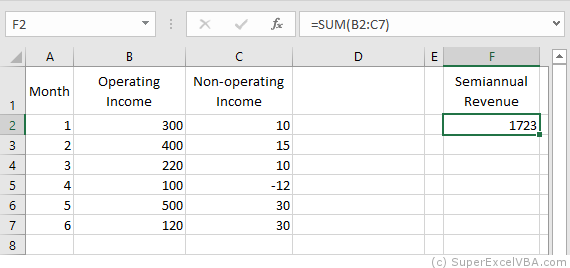
Formula adds predefined Excel formulas to the worksheet. These formulas should be written in English even if you have a language pack installed.
    Range("F2").Formula = "=SUM(B2:C7)"
    Range("F3").Formula = "=SUM($B$2:$C$7)"
Do not worry if the language of your Excel is not English because, as in the example, it will do the translation to the spreadsheet automatically.
Multiple formulas
You can insert multiple formulas at the same time using the Formula property. To do this, simply define a Range object that is larger than a single cell, and the predefined formula will be «dragged» across the range.
«Dragging» manually:
«Dragging» by VBA:
Range("D2:D7").Formula = "=SUM(B2:C2)"
Another way to perform the same action would be using FillDown method.
    Range("D2").Formula = "=SUM(B2:C2)"
    Range("D2:D7").FillDown
VBA FormulaLocal
FormulaLocal adds predefined Excel formulas to the worksheet. These formulas, however, should be written in the local language of Excel (in the case of Brazil, in Portuguese).
Range("F2").FormulaLocal = "=SOMA(B2:C7)"
Just as the Formula property, FormulaLocal can be used to make multiple formulas.
VBA FormulaR1C1
FormulaR1C1, as well as Formula and FormulaLocal, also adds pre-defined Excel formulas to the spreadsheet; however, the use of relative and absolute notations have different rules. The formula used must be written in English.
FormulaR1C1 is the way to use Excel’s ready-to-use formulas in VBA by easily integrating them into loops and counting variables.
In the notations:
- R refers to rows, in the case of vertical displacement
- C refers to columns, in the case of horizontal displacement
- N symbolizes an integer that indicates how much must be shifted in number of rows and/or columns
- Relative notation: Use as reference the Range that called it
The format of the relative formula is: R[N]C[N]:R[N]C[N].
    Range("F2").FormulaR1C1 = "=SUM(R[0]C[-4]:R[5]C[-3])" 'Equals the bottom row
    Range("F2").FormulaR1C1 = "=SUM(RC[-4]:R[5]C[-3])"
When N is omitted, the value 0 is assumed.
In the example, RC[-4]:R[5]C[-3] results in «B2: C7». These cells are obtained by: receding 4 columns to the left RC[-4] from Range(«F2») to obtain «B2»; and 5 lines down and 3 columns to the left R[5]C[-3] from Range(«F2») to obtain «C7».
- Absolute notation: Use the start of the spreadsheet as a reference
The format of the relative formula is: RNCN:RNCN.
Range("F2").FormulaR1C1 = "=SUM(R2C2:R7C3)" 'Results in "$B$2:$C$7"
N negative can only be used in relative notation.
The two notations (relative and absolute) can be merged.
Range("F2").FormulaR1C1 = "=SUM(RC[-4]:R7C3)" 'Results in "B2:$C$7"
VBA WorksheetFunction
Excel formulas can also be accessed by object WorksheetFunction methods.
Range("F2") = WorksheetFunction.Sum(Range("B2:C7"))
Excel formulas can also be accessed similarly to functions created in VBA.
The formulas present in the WorksheetFunction object are all in English.
One of the great advantages of accessing Excel formulas this way is to be able to use them more easily in the VBA environment.
    MsgBox (WorksheetFunction.Sum(3, 4, 5))
    Expense=4
    MsgBox (WorksheetFunction.Sum(3, 4, 5,-Expense))
To list the available Excel formulas in this format, simply type WorksheetFunction. that automatically an option menu with all formulas will appear:
Consolidating Your Learning
Suggested Exercise
SuperExcelVBA.com is learning website. Examples might be simplified to improve reading and basic understanding. Tutorials, references, and examples are constantly reviewed to avoid errors, but we cannot warrant full correctness of all content. All Rights Reserved.
Excel ® is a registered trademark of the Microsoft Corporation.
© 2023 SuperExcelVBA | ABOUT
![]()
In this Article
- Formulas in VBA
- Macro Recorder and Cell Formulas
- VBA FormulaR1C1 Property
- Absolute References
- Relative References
- Mixed References
- VBA Formula Property
- VBA Formula Tips
- Formula With Variable
- Formula Quotations
- Assign Cell Formula to String Variable
- Different Ways to Add Formulas to a Cell
- Refresh Formulas
This tutorial will teach you how to create cell formulas using VBA.
Formulas in VBA
Using VBA, you can write formulas directly to Ranges or Cells in Excel. It looks like this:
Sub Formula_Example()

    'Assign a hard-coded formula to a single cell
    Range("b3").Formula = "=b1+b2"

    'Assign a flexible formula to a range of cells
    Range("d1:d100").FormulaR1C1 = "=RC2+RC3"

End Sub
There are two Range properties you will need to know:
- .Formula – Creates an exact formula (hard-coded cell references). Good for adding a formula to a single cell.
- .FormulaR1C1 – Creates a flexible formula. Good for adding formulas to a range of cells where cell references should change.
For simple formulas, it’s fine to use the .Formula Property. However, for everything else, we recommend using the Macro Recorder…
Macro Recorder and Cell Formulas
The Macro Recorder is our go-to tool for writing cell formulas with VBA. You can simply:
- Start recording
- Type the formula (with relative / absolute references as needed) into the cell & press enter
- Stop recording
- Open VBA and review the formula, adapting as needed and copying+pasting the code where needed.
I find it’s much easier to enter a formula into a cell than to type the corresponding formula in VBA.
Notice a couple of things:
- The Macro Recorder will always use the .FormulaR1C1 property
- The Macro Recorder recognizes Absolute vs. Relative Cell References
VBA FormulaR1C1 Property
The FormulaR1C1 property uses R1C1-style cell referencing (as opposed to the standard A1-style you are accustomed to seeing in Excel).
Here are some examples:
Sub FormulaR1C1_Examples()

    'Reference D5 (Absolute)
    '=$D$5
    Range("a1").FormulaR1C1 = "=R5C4"

    'Reference D5 (Relative) from cell A1
    '=D5
    Range("a1").FormulaR1C1 = "=R[4]C[3]"

    'Reference D5 (Absolute Row, Relative Column) from cell A1
    '=D$5
    Range("a1").FormulaR1C1 = "=R5C[3]"

    'Reference D5 (Relative Row, Absolute Column) from cell A1
    '=$D5
    Range("a1").FormulaR1C1 = "=R[4]C4"

End Sub
Notice that the R1C1-style cell referencing allows you to set absolute or relative references.
Absolute References
In standard A1 notation an absolute reference looks like this: “=$C$2”. In R1C1 notation it looks like this: “=R2C3”.
To create an Absolute cell reference using R1C1-style type:
- R + Row number
- C + Column number
Example: R2C3 would represent cell $C$2 (C is the 3rd column).
    'Reference D5 (Absolute)
    '=$D$5
    Range("a1").FormulaR1C1 = "=R5C4"
Relative References
Relative cell references are cell references that “move” when the formula is moved.
In standard A1 notation they look like this: “=C2”. In R1C1 notation, you use brackets [] to offset the cell reference from the current cell.
Example: Entering formula “=R[1]C[1]” in cell B3 would reference cell D4 (the cell 1 row below and 1 column to the right of the formula cell).
Use negative numbers to reference cells above or to the left of the current cell.
    'Reference D5 (Relative) from cell A1
    '=D5
    Range("a1").FormulaR1C1 = "=R[4]C[3]"
Mixed References
Cell references can be partially relative and partially absolute. Example:
    'Reference D5 (Relative Row, Absolute Column) from cell A1
    '=$D5
    Range("a1").FormulaR1C1 = "=R[4]C4"
VBA Coding Made Easy
Stop searching for VBA code online. Learn more about AutoMacro — A VBA Code Builder that allows beginners to code procedures from scratch with minimal coding knowledge and with many time-saving features for all users!

Learn More
VBA Formula Property
When setting formulas with the .Formula Property you will always use A1-style notation. You enter the formula just like you would in an Excel cell, except surrounded by quotations:
    'Assign a hard-coded formula to a single cell
    Range("b3").Formula = "=b1+b2"
VBA Formula Tips
Formula With Variable
When working with Formulas in VBA, it’s very common to want to use variables within the cell formulas. To use variables, you use & to combine the variables with the rest of the formula string. Example:
Sub Formula_Variable()
    Dim colNum As Long
    colNum = 4

    Range("a1").FormulaR1C1 = "=R1C" & colNum & "+R2C" & colNum

End Sub
VBA Programming | Code Generator does work for you!
Formula Quotations
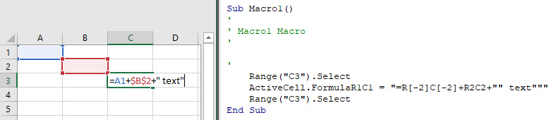
If you need to add a quotation (“) within a formula, enter the quotation twice (“”):
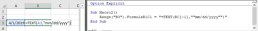
Sub Macro2()
    Range("B3").FormulaR1C1 = "=TEXT(RC[-1],""mm/dd/yyyy"")"
End Sub
A single quotation (“) signifies to VBA the end of a string of text. Whereas a double quotation (“”) is treated like a quotation within the string of text.
Similarly, use 3 quotation marks (“””) to surround a string with a quotation mark (“)
MsgBox """Use 3 to surround a string with quotes"""
' This will print <"Use 3 to surround a string with quotes"> immediate window
Assign Cell Formula to String Variable
We can read the formula in a given cell or range and assign it to a string variable:
'Assign Cell Formula to Variable
Dim strFormula as String
strFormula = Range("B1").Formula
Different Ways to Add Formulas to a Cell
Here are a few more examples for how to assign a formula to a cell:
- Directly Assign Formula
- Define a String Variable Containing the Formula
- Use Variables to Create Formula
Sub MoreFormulaExamples ()
' Alternate ways to add SUM formula
' to cell B1
'
  Dim strFormula as String
  Dim cell as Range
  dim fromRow as long, toRow as long

  Set cell = Range("B1")

  ' Directly assigning a String
  cell.Formula = "=SUM(A1:A10)"

  ' Storing string to a variable
  ' and assigning to "Formula" property
  strFormula = "=SUM(A1:A10)"
  cell.Formula = strFormula

  ' Using variables to build a string
  ' and assigning it to "Formula" property
  fromRow = 1
  toRow   = 10
  strFormula = "=SUM(A" & fromValue & ":A" & toValue & ")
  cell.Formula = strFormula
End Sub
Refresh Formulas
As a reminder, to refresh formulas, you can use the Calculate command:
CalculateTo refresh single formula, range, or entire worksheet use .Calculate instead:
Sheets("Sheet1").Range("a1:a10").CalculateВставка формулы со ссылками в стиле A1 и R1C1 в ячейку (диапазон) из кода VBA Excel. Свойства Range.FormulaLocal и Range.FormulaR1C1Local.
Свойство Range.FormulaLocal
FormulaLocal — это свойство объекта Range, которое возвращает или задает формулу на языке пользователя, используя ссылки в стиле A1.
В качестве примера будем использовать диапазон A1:E10, заполненный числами, которые необходимо сложить построчно и результат отобразить в столбце F:

Примеры вставки формул суммирования в ячейку F1:
|
Range(«F1»).FormulaLocal = «=СУММ(A1:E1)» Range(«F1»).FormulaLocal = «=СУММ(A1;B1;C1;D1;E1)» |
Пример вставки формул суммирования со ссылками в стиле A1 в диапазон F1:F10:
|
Sub Primer1() Dim i As Byte For i = 1 To 10 Range(«F» & i).FormulaLocal = «=СУММ(A» & i & «:E» & i & «)» Next End Sub |
В этой статье я не рассматриваю свойство Range.Formula, но если вы решите его применить для вставки формулы в ячейку, используйте англоязычные функции, а в качестве разделителей аргументов — запятые (,) вместо точек с запятой (;):
|
Range(«F1»).Formula = «=SUM(A1,B1,C1,D1,E1)» |
После вставки формула автоматически преобразуется в локальную (на языке пользователя).
Свойство Range.FormulaR1C1Local
FormulaR1C1Local — это свойство объекта Range, которое возвращает или задает формулу на языке пользователя, используя ссылки в стиле R1C1.
Формулы со ссылками в стиле R1C1 можно вставлять в ячейки рабочей книги Excel, в которой по умолчанию установлены ссылки в стиле A1. Вставленные ссылки в стиле R1C1 будут автоматически преобразованы в ссылки в стиле A1.
Примеры вставки формул суммирования со ссылками в стиле R1C1 в ячейку F1 (для той же таблицы):
|
‘Абсолютные ссылки в стиле R1C1: Range(«F1»).FormulaR1C1Local = «=СУММ(R1C1:R1C5)» Range(«F1»).FormulaR1C1Local = «=СУММ(R1C1;R1C2;R1C3;R1C4;R1C5)» ‘Ссылки в стиле R1C1, абсолютные по столбцам и относительные по строкам: Range(«F1»).FormulaR1C1Local = «=СУММ(RC1:RC5)» Range(«F1»).FormulaR1C1Local = «=СУММ(RC1;RC2;RC3;RC4;RC5)» ‘Относительные ссылки в стиле R1C1: Range(«F1»).FormulaR1C1Local = «=СУММ(RC[-5]:RC[-1])» Range(«F2»).FormulaR1C1Local = «=СУММ(RC[-5];RC[-4];RC[-3];RC[-2];RC[-1])» |
Пример вставки формул суммирования со ссылками в стиле R1C1 в диапазон F1:F10:
|
‘Ссылки в стиле R1C1, абсолютные по столбцам и относительные по строкам: Range(«F1:F10»).FormulaR1C1Local = «=СУММ(RC1:RC5)» ‘Относительные ссылки в стиле R1C1: Range(«F1:F10»).FormulaR1C1Local = «=СУММ(RC[-5]:RC[-1])» |
Так как формулы с относительными ссылками и относительными по строкам ссылками в стиле R1C1 для всех ячеек столбца F одинаковы, их можно вставить сразу, без использования цикла, во весь диапазон.
In this lesson you can learn how to add a formula to a cell using vba. There are several ways to insert formulas to cells automatically. We can use properties like Formula, Value and FormulaR1C1 of the Range object. This post explains five different ways to add formulas to cells.
Table of contents
How to add formula to cell using VBA
Add formula to cell and fill down using VBA
Add sum formula to cell using VBA
How to add If formula to cell using VBA
Add formula to cell with quotes using VBA
Add Vlookup formula to cell using VBA
We use formulas to calculate various things in Excel. Sometimes you may need to enter the same formula to hundreds or thousands of rows or columns only changing the row numbers or columns. For an example let’s consider this sample Excel sheet.
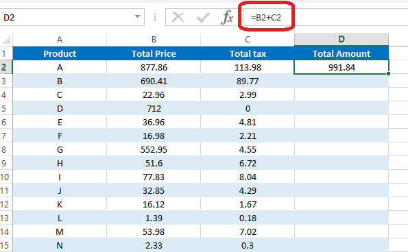
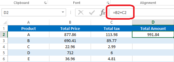
In this Excel sheet I have added a very simple formula to the D2 cell.
=B2+C2
So what if we want to add similar formulas for all the rows in column D. So the D3 cell will have the formula as =B3+C3 and D4 will have the formula as =B4+D4 and so on. Luckily we don’t need to type the formulas manually in all rows. There is a much easier way to do this. First select the cell containing the formula. Then take the cursor to the bottom right corner of the cell. Mouse pointer will change to a + sign. Then left click and drag the mouse until the end of the rows.
However if you want to add the same formula again and again for lots of Excel sheets then you can use a VBA macro to speed up the process. First let’s look at how to add a formula to one cell using vba.
How to add formula to cell using VBA
Lets see how we can enter above simple formula(=B2+C2) to cell D2 using VBA
In this method we are going to use the Formula property of the Range object.
Sub AddFormula_Method1()
Dim WS As Worksheet
Set WS = Worksheets(«Sheet1»)
WS.Range(«D2»).Formula = «=B2+C2»
End Sub
We can also use the Value property of the Range object to add a formula to a cell.
Sub AddFormula_Method2()
Dim WS As Worksheet
Set WS = Worksheets(«Sheet1»)
WS.Range(«D2»).Value = «=B2+C2»
End Sub
Next method is to use the FormulaR1C1 property of the Range object. There are few different ways to use FormulaR1C1 property. We can use absolute reference, relative reference or use both types of references inside the same formula.
In the absolute reference method cells are referred to using numbers. Excel sheets have numbers for each row. So you should think similarly for columns. So column A is number 1. Column B is number 2 etc. Then when writing the formula use R before the row number and C before the column number. So the cell A1 is referred to by R1C1. A2 is referred to by R2C1. B3 is referred to by R3C2 etc.
This is how you can use the absolute reference.
Sub AddFormula_Method3A()
Dim WS As Worksheet
Set WS = Worksheets(«Sheet1»)
WS.Range(«D2»).FormulaR1C1 = «=R2C2+R2C3»
End Sub
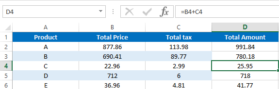
If you use the absolute reference, the formula will be added like this.
If you use the manual drag method explained above to fill down other rows, then the same formula will be copied to all the rows.
In Majority cases this is not how you want to fill down the formula. However this won’t happen in the relative method. In the relative method, cells are given numbers relative to the cell where the formula is entered. You should use negative numbers when referring to the cells in upward direction or left. Also the numbers should be placed within the square brackets. And you can omit [0] when referring to cells on the same row or column. So you can use RC[-2] instead of R[0]C[-2]. The macro recorder also generates relative reference type code, if you enter a formula to a cell while enabling the macro recorder.
Below example shows how to put formula =B2+C2 in D2 cell using relative reference method.
Sub AddFormula_Method3B()
Dim WS As Worksheet
Set WS = Worksheets(«Sheet1»)
WS.Range(«D2»).FormulaR1C1 = «=RC[-2]+RC[-1]»
End Sub
Now use the drag method to fill down all the rows.
You can see that the formulas are changed according to the row numbers.
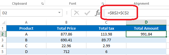
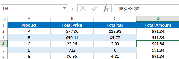
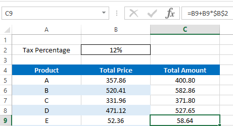
Also you can use both relative and absolute references in the same formula. Here is a typical example where you need a formula with both reference types.
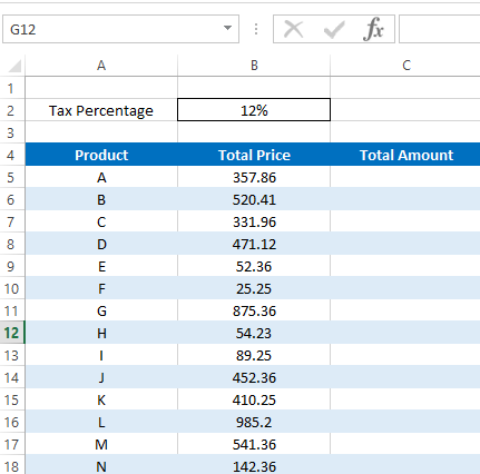
We can add the formula to calculate Total Amount like this.
Sub AddFormula_Method3C()
Dim WS As Worksheet
Set WS = Worksheets(«Sheet2»)
WS.Range(«C5»).FormulaR1C1 = «=RC[-1]+RC[-1]*R2C2»
End Sub
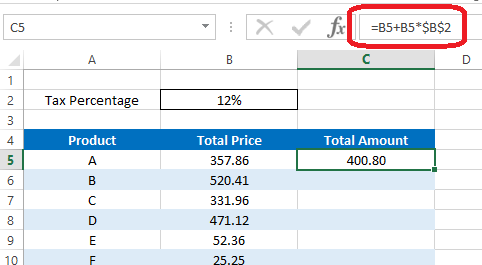
In this formula we have a absolute reference after the * symbol. So when we fill down the formula using the drag method that part will remain the same for all the rows. Hence we will get correct results for all the rows.
Add formula to cell and fill down using VBA
So now you’ve learnt various methods to add a formula to a cell. Next let’s look at how to fill down the other rows with the added formula using VBA.
Assume we have to calculate cell D2 value using =B2+C2 formula and fill down up to 1000 rows. First let’s see how we can modify the first method to do this. Let’s name this subroutine as “AddFormula_Method1_1000Rows”
Sub AddFormula_Method1_1000Rows()
End Sub
Then we need an additional variable for the For Next statement
Dim WS As Worksheet
Dim i As Integer
Next, assign the worksheet to WS variable
Set WS = Worksheets(«Sheet1»)
Now we can add the For Next statement like this.
For i = 2 To 1000
WS.Range(«D» & i).Formula = «=B» & i & «+C» & i
Next i
Here I have used «D» & i instead of D2 and «=B» & i & «+C» & i instead of «=B2+C2». So the formula keeps changing like =B3+C3, =B4+C4, =B5+C5 etc. when iterated through the For Next loop.
Below is the full code of the subroutine.
Sub AddFormula_Method1_1000Rows()
Dim WS As Worksheet
Dim i As Integer
Set WS = Worksheets(«Sheet1»)
For i = 2 To 1000
WS.Range(«D» & i).Formula = «=B» & i & «+C» & i
Next i
End Sub
So that’s how you can use VBA to add formulas to cells with variables.
Next example shows how to modify the absolute reference type of FormulaR1C1 method to add formulas upto 1000 rows.
Sub AddFormula_Method3A_1000Rows()
Dim WS As Worksheet
Dim i As Integer
Set WS = Worksheets(«Sheet1»)
For i = 2 To 1000
WS.Range(«D» & i).FormulaR1C1 = «=R» & i & «C2+R» & i & «C3»
Next i
End Sub
You don’t need to do any change to the formula section when modifying the relative reference type of the FormulaR1C1 method.
Sub AddFormula_Method3B_1000Rows()
Dim WS As Worksheet
Dim i As Integer
Set WS = Worksheets(«Sheet1»)
For i = 2 To 1000
WS.Range(«D» & i).FormulaR1C1 = «=RC[-2]+RC[-1]»
Next i
End Sub
Use similar techniques to modify other two types of subroutines to add formulas for multiple rows. Now you know how to add formulas to cells with a variable. Next let’s look at how to add formulas with some inbuilt functions using VBA.
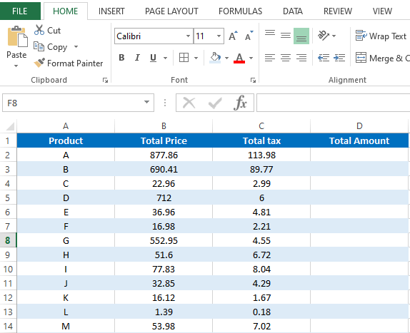
How to add sum formula to a cell using VBA
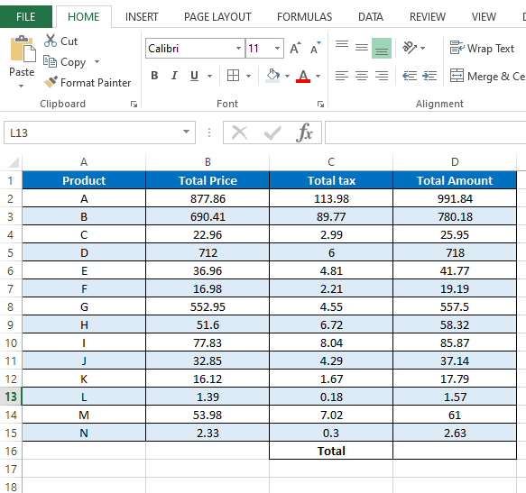
Suppose we want the total of column D in the D16 cell. So this is the formula we need to create.
=SUM(D2:D15)
Now let’s see how to add this using VBA. Let’s name this subroutine as SumFormula.
First let’s declare a few variables.
Dim WS As Worksheet
Dim StartingRow As Long
Dim EndingRow As Long
Assign the worksheet to the variable.
Set WS = Worksheets(«Sheet3»)
Assign the starting row and the ending row to relevant variables.
StartingRow = 2
EndingRow = 1
Then the final step is to create the formula with the above variables.
WS.Range(«D16»).Formula = «=SUM(D» & StartingRow & «:D» & EndingRow & «)»
Below is the full code to add the Sum formula using VBA.
Sub SumFormula()
Dim WS As Worksheet
Dim StartingRow As Long
Dim EndingRow As Long
Set WS = Worksheets(«Sheet3»)
StartingRow = 2
EndingRow = 15
WS.Range(«D16»).Formula = «=SUM(D» & StartingRow & «:D» & EndingRow & «)»
End Sub
How to add If Formula to a cell using VBA
If function is a very popular inbuilt worksheet function available in Microsoft Excel. This function has 3 arguments. Two of them are optional.
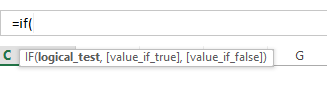
Now let’s see how to add a If formula to a cell using VBA. Here is a typical example where we need a simple If function.
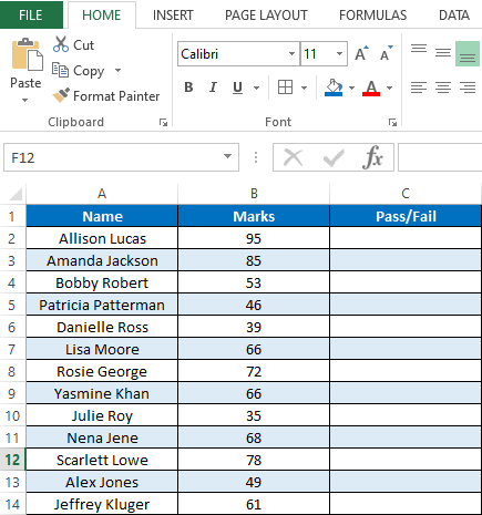
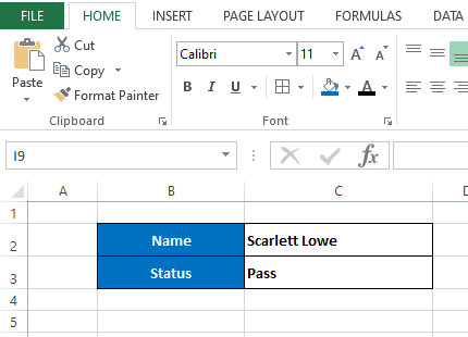
This is the results of students on an examination. Here we have names of students in column A and their marks in column B. Students should get “Pass” if he/she has marks equal or higher than 40. If marks are less than 40 then Excel should show the “Fail” in column C. We can simply obtain this result by adding an If function to column C. Below is the function we need in the C2 cell.
=IF(B2>=40,»Pass»,»Fail»)
Now let’s look at how to add this If Formula to a C2 cell using VBA. Once you know how to add it then you can use the For Next statement to fill the rest of the rows like we did above. We discussed a few different ways to add formulas to a range object using VBA. For this particular example I’m going to use the Formula property of the Range object.
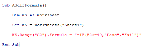
So now let’s see how we can develop this macro. Let’s name this subroutine as “AddIfFormula”
Sub AddIfFormula()
End Sub
However we can’t simply add this If formula using the Formula property like we did before. Because this If formula has quotes inside it. So if we try to add the formula to the cell with quotes, then we get a syntax error.
Add formula to cell with quotes
There are two ways to add the formula to a cell with quotes.
Sub AddIfFormula_Method1()
Dim WS As Worksheet
Set WS = Worksheets(«Sheet4»)
WS.Range(«C2»).Formula = «=IF(B2>=40,»»Pass»»,»»Fail»»)»
End Sub
Sub AddIfFormula_Method2()
Dim WS As Worksheet
Set WS = Worksheets(«Sheet4»)
WS.Range(«C2»).Formula = «=IF(B2>=40,» & Chr(34) & «Pass» & Chr(34) & «,» & Chr(34) & «Fail» & Chr(34) & «)»
End Sub
Add vlookup formula to cell using VBA
Finally I will show you how to add a vlookup formula to a cell using VBA. So I created a very simple example where we can use a Vlookup function. Assume we have this section in the Sheet5 of the same workbook.
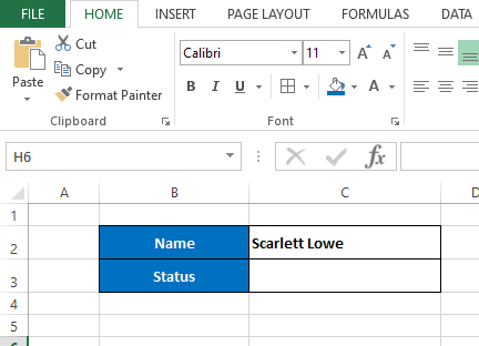
So here when we change the name of the student in the C2 cell, his/her pass or fail status should automatically be shown in the C3 cell. If the original data(data we used in the above “If formula” example) is listed in the Sheet4 then we can write a Vlookup formula for the C3 cell like this.
=VLOOKUP(Sheet5!C2,Sheet4!A2:C200,3,FALSE)
We can use the Formula property of the Range object to add this Vlookup formula to the C3 using VBA.
Sub AddVlookupFormula()
Dim WS As Worksheet
Set WS = Worksheets(«Sheet5»)
WS.Range(«C3»).Formula = «=VLOOKUP(Sheet5!C2,Sheet4!A2:C200,3,FALSE)»
End Sub
Home / VBA / VBA Calculate (Cell, Range, Row, & Workbook)
By default, in Excel, whenever you change a cell value Excel recalculates all the cells that have a calculation dependency on that cell. But when you are using VBA, you have an option to change it to the manual, just like we do in Excel.

Using VBA Calculate Method
You can change the calculation to the manual before you start a code, just like the following.
Application.Calculation = xlManualWhen you run this code, it changes the calculation to manual.

And at the end of the code, you can use the following line of code to switch to the automatic.
Application.Calculation = xlAutomatic
You can use calculation in the following way.

Sub myMacro()
    Application.Calculation = xlManual
        'your code goes here
    Application.Calculation = xlAutomatic
End Sub
Calculate Now (All the Open Workbooks)
If you simply want to re-calculate all the open workbooks, you can use the “Calculate” method just like below.
CalculateUse Calculate Method for a Sheet
Using the following way, you can re-calculate all the calculations for all the
ActiveSheet.Calculate
Sheets("Sheet1").Calculate
The first line of code re-calculates for the active sheet and the second line does it for the “Sheet1” but you can change the sheet if you want.
Calculate for a Range or a Single Cell
In the same way, you can re-calculate all the calculations for a particular range or a single cell, just like the following.
Sheets("Sheet1").Range("A1:A10").Calculate
Sheets("Sheet1").Range("A1").Calculate
Содержание
- Итоговый рабочий лист
- Присвоение результата суммы переменной

- Суммировать объект диапазона
- Суммировать несколько объектов диапазона
- Суммировать весь столбец или строку
- Суммировать массив
- Использование функции SumIf
- Формула суммы

Из этого туториала Вы узнаете, как использовать функцию Excel Sum в VBA.
Функция суммы — одна из наиболее широко используемых функций Excel и, вероятно, первая, которую пользователи Excel научились использовать. VBA фактически не имеет эквивалента — пользователь должен использовать встроенную функцию Excel в VBA, используя Рабочий лист объект.
Итоговый рабочий лист
Объект WorksheetFunction можно использовать для вызова большинства функций Excel, доступных в диалоговом окне «Вставить функцию» в Excel. Функция СУММ — одна из них.
| 123 | Sub TestFunctionДиапазон («D33») = Application.WorksheetFunction.Sum («D1: D32»)Конец подписки |

В функции СУММ может быть до 30 аргументов. Каждый из аргументов также может относиться к диапазону ячеек.
В этом примере ниже добавляются ячейки с D1 по D9.
| 123 | Sub TestSum ()Диапазон («D10») = Application.WorksheetFunction.SUM («D1: D9»)Конец подписки |
В приведенном ниже примере добавляется диапазон в столбце D и диапазон в столбце F. Если вы не введете объект Application, он будет принят.
| 123 | Sub TestSum ()Диапазон («D25») = WorksheetFunction.SUM (Диапазон («D1: D24»), Диапазон («F1: F24»))Конец подписки |
Обратите внимание, что для одного диапазона ячеек вам не нужно указывать слово «Диапазон» в формуле перед ячейками, это предполагается кодом. Однако, если вы используете несколько аргументов, вам нужно это сделать.
Присвоение результата суммы переменной
Возможно, вы захотите использовать результат своей формулы в другом месте кода, а не записывать его непосредственно обратно в Excel Range. В этом случае вы можете присвоить результат переменной, которая будет использоваться позже в вашем коде.
| 1234567 | Sub AssignSumVariable ()Тусклый результат как двойной’Назначьте переменнуюрезультат = WorksheetFunction.SUM (Диапазон («G2: G7»), Диапазон («H2: H7»))’Показать результатMsgBox «Всего диапазонов» & результатКонец подписки |
Суммировать объект диапазона
Вы можете назначить группу ячеек объекту Range, а затем использовать этот объект Range с Рабочий лист объект.
| 123456789 | Sub TestSumRange ()Dim rng As Range’назначить диапазон ячеекУстановить rng = Range («D2: E10»)’используйте диапазон в формулеДиапазон («E11») = WorksheetFunction.SUM (rng)’отпустить объект диапазонаУстановить rng = ничегоКонец подписки |
Суммировать несколько объектов диапазона
Точно так же вы можете суммировать несколько объектов диапазона.
| 123456789101112 | Sub TestSumMultipleRanges ()Dim rngA As ДиапазонDim rngB as Range’назначить диапазон ячеекУстановите rngA = Range («D2: D10»)Установите rngB = Range («E2: E10»)’используйте диапазон в формулеДиапазон («E11») = WorksheetFunction.SUM (rngA, rngB)’отпустить объект диапазонаУстановите rngA = NothingУстановить rngB = НичегоКонец подписки |
Суммировать весь столбец или строку
Вы также можете использовать функцию Sum, чтобы сложить весь столбец или всю строку
Эта процедура ниже суммирует все числовые ячейки в столбце D.
| 123 | Sub TestSum ()Диапазон («F1») = WorksheetFunction.SUM (Диапазон («D: D»)Конец подписки |
В то время как эта процедура ниже суммирует все числовые ячейки в строке 9.
| 123 | Sub TestSum ()Диапазон («F2») = WorksheetFunction.SUM (Диапазон («9: 9»)Конец подписки |
Суммировать массив
Вы также можете использовать WorksheetFunction.Sum для суммирования значений в массиве.
| 123456789101112 | Sub TestArray ()Dim intA (от 1 до 5) как целое числоDim SumArray как целое число’заполнить массивintA (1) = 15intA (2) = 20intA (3) = 25intA (4) = 30intA (5) = 40’сложите массив и покажите результатMsgBox WorksheetFunction.SUM (intA)Конец подписки |
Использование функции SumIf
Еще одна функция рабочего листа, которую можно использовать, — это функция СУММЕСЛИ.
| 123 | Sub TestSumIf ()Диапазон («D11») = WorksheetFunction.SUMIF (Диапазон («C2: C10»), 150, Диапазон («D2: D10»))Конец подписки |
Приведенная выше процедура суммирует только ячейки в диапазоне (D2: D10), если соответствующая ячейка в столбце C = 150.

Формула суммы
Когда вы используете Рабочий лист Функция. СУММ чтобы добавить сумму к диапазону на листе, возвращается статическая сумма, а не гибкая формула. Это означает, что при изменении ваших цифр в Excel значение, возвращаемое Рабочий лист не изменится.

В приведенном выше примере процедура TestSum суммировала диапазон (D2: D10), и результат был помещен в D11. Как вы можете видеть в строке формул, это число, а не формула.
Если любое из значений изменится в диапазоне (D2: D10), результат в D11 будет НЕТ изменение.
Вместо использования Рабочий лист Функция. СУММ, вы можете использовать VBA для применения функции суммы к ячейке с помощью Формула или Формула R1C1 методы.
Формула Метод
Метод формулы позволяет указать конкретный диапазон ячеек, например: D2: D10, как показано ниже.
| 123 | Sub TestSumFormulaДиапазон («D11»). Формула = «= СУММ (D2: D10)»Конец подписки |

Метод FormulaR1C1
Метод FromulaR1C1 более гибкий, поскольку он не ограничивает вас заданным диапазоном ячеек. Пример ниже даст нам тот же ответ, что и приведенный выше.
| 123 | Sub TestSumFormula ()Диапазон («D11»). FormulaR1C1 = «= СУММ (R [-9] C: R [-1] C)»Конец подписки |

Однако, чтобы сделать формулу более гибкой, мы могли бы изменить код, чтобы он выглядел так:
| 123 | Sub TestSumFormula ()ActiveCell.FormulaR1C1 = «= СУММ (R [-9] C: R [-1] C)»Конец подписки |
Где бы вы ни находились на своем листе, формула складывает 8 ячеек прямо над ней и помещает ответ в вашу ActiveCell. На диапазон внутри функции SUM следует ссылаться с использованием синтаксиса Row (R) и Column (C).
Оба эти метода позволяют использовать динамические формулы Excel в VBA.
Теперь вместо значения в D11 будет формула.