
Свойства ячейки, часто используемые в коде VBA Excel. Демонстрация свойств ячейки, как структурной единицы объекта Range, на простых примерах.
Объект Range в VBA Excel представляет диапазон ячеек. Он (объект Range) может описывать любой диапазон, начиная от одной ячейки и заканчивая сразу всеми ячейками рабочего листа.
Примеры диапазонов:
- Одна ячейка –
Range("A1"). - Девять ячеек –
Range("A1:С3"). - Весь рабочий лист в Excel 2016 –
Range("1:1048576").
Для справки: выражение Range("1:1048576") описывает диапазон с 1 по 1048576 строку, где число 1048576 – это номер последней строки на рабочем листе Excel 2016.
В VBA Excel есть свойство Cells объекта Range, которое позволяет обратиться к одной ячейке в указанном диапазоне (возвращает объект Range в виде одной ячейки). Если в коде используется свойство Cells без указания диапазона, значит оно относится ко всему диапазону активного рабочего листа.
Примеры обращения к одной ячейке:
Cells(1000), где 1000 – порядковый номер ячейки на рабочем листе, возвращает ячейку «ALL1».Cells(50, 20), где 50 – номер строки рабочего листа, а 20 – номер столбца, возвращает ячейку «T50».Range("A1:C3").Cells(6), где «A1:C3» – заданный диапазон, а 6 – порядковый номер ячейки в этом диапазоне, возвращает ячейку «C2».
Для справки: порядковый номер ячейки в диапазоне считается построчно слева направо с перемещением к следующей строке сверху вниз.
Подробнее о том, как обратиться к ячейке, смотрите в статье: Ячейки (обращение, запись, чтение, очистка).
В этой статье мы рассмотрим свойства объекта Range, применимые, в том числе, к диапазону, состоящему из одной ячейки.
Еще надо добавить, что свойства и методы объектов отделяются от объектов точкой, как в третьем примере обращения к одной ячейке: Range("A1:C3").Cells(6).
Свойства ячейки (объекта Range)
| Свойство | Описание |
|---|---|
| Address | Возвращает адрес ячейки (диапазона). |
| Borders | Возвращает коллекцию Borders, представляющую границы ячейки (диапазона). Подробнее… |
| Cells | Возвращает объект Range, представляющий коллекцию всех ячеек заданного диапазона. Указав номер строки и номер столбца или порядковый номер ячейки в диапазоне, мы получаем конкретную ячейку. Подробнее… |
| Characters | Возвращает подстроку в размере указанного количества символов из текста, содержащегося в ячейке. Подробнее… |
| Column | Возвращает номер столбца ячейки (первого столбца диапазона). Подробнее… |
| ColumnWidth | Возвращает или задает ширину ячейки в пунктах (ширину всех столбцов в указанном диапазоне). |
| Comment | Возвращает комментарий, связанный с ячейкой (с левой верхней ячейкой диапазона). |
| CurrentRegion | Возвращает прямоугольный диапазон, ограниченный пустыми строками и столбцами. Очень полезное свойство для возвращения рабочей таблицы, а также определения номера последней заполненной строки. |
| EntireColumn | Возвращает весь столбец (столбцы), в котором содержится ячейка (диапазон). Диапазон может содержаться и в одном столбце, например, Range("A1:A20"). |
| EntireRow | Возвращает всю строку (строки), в которой содержится ячейка (диапазон). Диапазон может содержаться и в одной строке, например, Range("A2:H2"). |
| Font | Возвращает объект Font, представляющий шрифт указанного объекта. Подробнее о цвете шрифта… |
| HorizontalAlignment | Возвращает или задает значение горизонтального выравнивания содержимого ячейки (диапазона). Подробнее… |
| Interior | Возвращает объект Interior, представляющий внутреннюю область ячейки (диапазона). Применяется, главным образом, для возвращения или назначения цвета заливки (фона) ячейки (диапазона). Подробнее… |
| Name | Возвращает или задает имя ячейки (диапазона). |
| NumberFormat | Возвращает или задает код числового формата для ячейки (диапазона). Примеры кодов числовых форматов можно посмотреть, открыв для любой ячейки на рабочем листе Excel диалоговое окно «Формат ячеек», на вкладке «(все форматы)». Свойство NumberFormat диапазона возвращает значение NULL, за исключением тех случаев, когда все ячейки в диапазоне имеют одинаковый числовой формат. Если нужно присвоить ячейке текстовый формат, записывается так: Range("A1").NumberFormat = "@". Общий формат: Range("A1").NumberFormat = "General". |
| Offset | Возвращает объект Range, смещенный относительно первоначального диапазона на указанное количество строк и столбцов. Подробнее… |
| Resize | Изменяет размер первоначального диапазона до указанного количества строк и столбцов. Строки добавляются или удаляются снизу, столбцы – справа. Подробнее… |
| Row | Возвращает номер строки ячейки (первой строки диапазона). Подробнее… |
| RowHeight | Возвращает или задает высоту ячейки в пунктах (высоту всех строк в указанном диапазоне). |
| Text | Возвращает форматированный текст, содержащийся в ячейке. Свойство Text диапазона возвращает значение NULL, за исключением тех случаев, когда все ячейки в диапазоне имеют одинаковое содержимое и один формат. Предназначено только для чтения. Подробнее… |
| Value | Возвращает или задает значение ячейки, в том числе с отображением значений в формате Currency и Date. Тип данных Variant. Value является свойством ячейки по умолчанию, поэтому в коде его можно не указывать. |
| Value2 | Возвращает или задает значение ячейки. Тип данных Variant. Значения в формате Currency и Date будут отображены в виде чисел с типом данных Double. |
| VerticalAlignment | Возвращает или задает значение вертикального выравнивания содержимого ячейки (диапазона). Подробнее… |
В таблице представлены не все свойства объекта Range. С полным списком вы можете ознакомиться не сайте разработчика.
Простые примеры для начинающих
Вы можете скопировать примеры кода VBA Excel в стандартный модуль и запустить их на выполнение. Как создать стандартный модуль и запустить процедуру на выполнение, смотрите в статье VBA Excel. Начинаем программировать с нуля.
Учтите, что в одном программном модуле у всех процедур должны быть разные имена. Если вы уже копировали в модуль подпрограммы с именами Primer1, Primer2 и т.д., удалите их или создайте еще один стандартный модуль.
Форматирование ячеек
Заливка ячейки фоном, изменение высоты строки, запись в ячейки текста, автоподбор ширины столбца, выравнивание текста в ячейке и выделение его цветом, добавление границ к ячейкам, очистка содержимого и форматирования ячеек.
Если вы запустите эту процедуру, информационное окно MsgBox будет прерывать выполнение программы и сообщать о том, что произойдет дальше, после его закрытия.
|
1 2 3 4 5 6 7 8 9 10 11 12 13 14 15 16 17 18 19 20 21 22 23 24 25 26 27 28 29 30 31 32 33 34 35 36 37 38 |
Sub Primer1() MsgBox «Зальем ячейку A1 зеленым цветом и запишем в ячейку B1 текст: «Ячейка A1 зеленая!»» Range(«A1»).Interior.Color = vbGreen Range(«B1»).Value = «Ячейка A1 зеленая!» MsgBox «Сделаем высоту строки, в которой находится ячейка A2, в 2 раза больше высоты ячейки A1, « _ & «а в ячейку B1 вставим текст: «Наша строка стала в 2 раза выше первой строки!»» Range(«A2»).RowHeight = Range(«A1»).RowHeight * 2 Range(«B2»).Value = «Наша строка стала в 2 раза выше первой строки!» MsgBox «Запишем в ячейку A3 высоту 2 строки, а в ячейку B3 вставим текст: «Такова высота второй строки!»» Range(«A3»).Value = Range(«A2»).RowHeight Range(«B3»).Value = «Такова высота второй строки!» MsgBox «Применим к столбцу, в котором содержится ячейка B1, метод AutoFit для автоподбора ширины» Range(«B1»).EntireColumn.AutoFit MsgBox «Выделим текст в ячейке B2 красным цветом и выровним его по центру (по вертикали)» Range(«B2»).Font.Color = vbRed Range(«B2»).VerticalAlignment = xlCenter MsgBox «Добавим к ячейкам диапазона A1:B3 границы» Range(«A1:B3»).Borders.LineStyle = True MsgBox «Сделаем границы ячеек в диапазоне A1:B3 двойными» Range(«A1:B3»).Borders.LineStyle = xlDouble MsgBox «Очистим ячейки диапазона A1:B3 от заливки, выравнивания, границ и содержимого» Range(«A1:B3»).Clear MsgBox «Присвоим высоте второй строки высоту первой, а ширине второго столбца — ширину первого» Range(«A2»).RowHeight = Range(«A1»).RowHeight Range(«B1»).ColumnWidth = Range(«A1»).ColumnWidth MsgBox «Демонстрация форматирования ячеек закончена!» End Sub |
Вычисления в ячейках (свойство Value)
Запись двух чисел в ячейки, вычисление их произведения, вставка в ячейку формулы, очистка ячеек.
Обратите внимание, что разделителем дробной части у чисел в VBA Excel является точка, а не запятая.
|
1 2 3 4 5 6 7 8 9 10 11 12 13 14 15 16 17 18 19 20 21 22 23 24 |
Sub Primer2() MsgBox «Запишем в ячейку A1 число 25.3, а в ячейку B1 — число 34.42» Range(«A1»).Value = 25.3 Range(«B1»).Value = 34.42 MsgBox «Запишем в ячейку C1 произведение чисел, содержащихся в ячейках A1 и B1» Range(«C1»).Value = Range(«A1»).Value * Range(«B1»).Value MsgBox «Запишем в ячейку D1 формулу, которая перемножает числа в ячейках A1 и B1» Range(«D1»).Value = «=A1*B1» MsgBox «Заменим содержимое ячеек A1 и B1 на числа 6.258 и 54.1, а также активируем ячейку D1» Range(«A1»).Value = 6.258 Range(«B1»).Value = 54.1 Range(«D1»).Activate MsgBox «Мы видим, что в ячейке D1 произведение изменилось, а в строке состояния отображается формула; « _ & «следующим шагом очищаем задействованные ячейки» Range(«A1:D1»).Clear MsgBox «Демонстрация вычислений в ячейках завершена!» End Sub |
Так как свойство Value является свойством ячейки по умолчанию, его можно было нигде не указывать. Попробуйте удалить .Value из всех строк, где оно встречается и запустить код заново.
Различие свойств Text, Value и Value2
Построение с помощью кода VBA Excel таблицы с результатами сравнения того, как свойства Text, Value и Value2 возвращают число, дату и текст.
|
1 2 3 4 5 6 7 8 9 10 11 12 13 14 15 16 17 18 19 20 21 22 23 24 25 26 27 28 29 30 31 32 33 34 35 36 37 38 39 40 41 42 43 44 45 46 47 48 49 50 51 52 53 54 55 56 |
Sub Primer3() ‘Присваиваем ячейкам всей таблицы общий формат на тот ‘случай, если формат отдельных ячеек ранее менялся Range(«A1:E4»).NumberFormat = «General» ‘добавляем сетку (границы ячеек) Range(«A1:E4»).Borders.LineStyle = True ‘Создаем строку заголовков Range(«A1») = «Значение» Range(«B1») = «Код формата» ‘формат соседней ячейки в столбце A Range(«C1») = «Свойство Text» Range(«D1») = «Свойство Value» Range(«E1») = «Свойство Value2» ‘Назначаем строке заголовков жирный шрифт Range(«A1:E1»).Font.Bold = True ‘Задаем форматы ячейкам A2, A3 и A4 ‘Ячейка A2 — числовой формат с разделителем триад и двумя знаками после запятой ‘Ячейка A3 — формат даты «ДД.ММ.ГГГГ» ‘Ячейка A4 — текстовый формат Range(«A2»).NumberFormat = «# ##0.00» Range(«A3»).NumberFormat = «dd.mm.yyyy» Range(«A4»).NumberFormat = «@» ‘Заполняем ячейки A2, A3 и A4 значениями Range(«A2») = 2362.4568 Range(«A3») = CDate(«01.01.2021») ‘Функция CDate преобразует текстовый аргумент в формат даты Range(«A4») = «Озеро Байкал» ‘Заполняем ячейки B2, B3 и B4 кодами форматов соседних ячеек в столбце A Range(«B2») = Range(«A2»).NumberFormat Range(«B3») = Range(«A3»).NumberFormat Range(«B4») = Range(«A4»).NumberFormat ‘Присваиваем ячейкам C2-C4 значения свойств Text ячеек A2-A4 Range(«C2») = Range(«A2»).Text Range(«C3») = Range(«A3»).Text Range(«C4») = Range(«A4»).Text ‘Присваиваем ячейкам D2-D4 значения свойств Value ячеек A2-A4 Range(«D2») = Range(«A2»).Value Range(«D3») = Range(«A3»).Value Range(«D4») = Range(«A4»).Value ‘Присваиваем ячейкам E2-E4 значения свойств Value2 ячеек A2-A4 Range(«E2») = Range(«A2»).Value2 Range(«E3») = Range(«A3»).Value2 Range(«E4») = Range(«A4»).Value2 ‘Применяем к таблице автоподбор ширины столбцов Range(«A1:E4»).EntireColumn.AutoFit End Sub |
Результат работы кода:

В таблице наглядно видна разница между свойствами Text, Value и Value2 при применении их к ячейкам с отформатированным числом и датой. Свойство Text еще отличается от Value и Value2 тем, что оно предназначено только для чтения.
Formatting Cells Number
General
Range("A1").NumberFormat = "General"Number
Range("A1").NumberFormat = "0.00"Currency
Range("A1").NumberFormat = "$#,##0.00"Accounting
Range("A1").NumberFormat = "_($* #,##0.00_);_($* (#,##0.00);_($* ""-""??_);_(@_)"Date
Range("A1").NumberFormat = "yyyy-mm-dd;@"Time
Range("A1").NumberFormat = "h:mm:ss AM/PM;@"Percentage
Range("A1").NumberFormat = "0.00%"Fraction
Range("A1").NumberFormat = "# ?/?"Scientific
Range("A1").NumberFormat = "0.00E+00"Text
Range("A1").NumberFormat = "@"Special
Range("A1").NumberFormat = "00000"Custom
Range("A1").NumberFormat = "$#,##0.00_);[Red]($#,##0.00)"Formatting Cells Alignment
Text Alignment
Horizontal
The value of this property can be set to one of the constants: xlGeneral, xlCenter, xlDistributed, xlJustify, xlLeft, xlRight.
The following code sets the horizontal alignment of cell A1 to center.
Range("A1").HorizontalAlignment = xlCenterVertical
The value of this property can be set to one of the constants: xlBottom, xlCenter, xlDistributed, xlJustify, xlTop.
The following code sets the vertical alignment of cell A1 to bottom.
Range("A1").VerticalAlignment = xlBottomText Control
Wrap Text
This example formats cell A1 so that the text wraps within the cell.
Range("A1").WrapText = TrueShrink To Fit
This example causes text in row one to automatically shrink to fit in the available column width.
Rows(1).ShrinkToFit = TrueMerge Cells
This example merge range A1:A4 to a large one.
Range("A1:A4").MergeCells = TrueRight-to-left
Text direction
The value of this property can be set to one of the constants: xlRTL (right-to-left), xlLTR (left-to-right), or xlContext (context).
The following code example sets the reading order of cell A1 to xlRTL (right-to-left).
Range("A1").ReadingOrder = xlRTLOrientation
The value of this property can be set to an integer value from –90 to 90 degrees or to one of the following constants: xlDownward, xlHorizontal, xlUpward, xlVertical.
The following code example sets the orientation of cell A1 to xlHorizontal.
Range("A1").Orientation = xlHorizontalFont
Font Name
The value of this property can be set to one of the fonts: Calibri, Times new Roman, Arial…
The following code sets the font name of range A1:A5 to Calibri.
Range("A1:A5").Font.Name = "Calibri"Font Style
The value of this property can be set to one of the constants: Regular, Bold, Italic, Bold Italic.
The following code sets the font style of range A1:A5 to Italic.
Range("A1:A5").Font.FontStyle = "Italic"Font Size
The value of this property can be set to an integer value from 1 to 409.
The following code sets the font size of cell A1 to 14.
Range("A1").Font.Size = 14Underline
The value of this property can be set to one of the constants: xlUnderlineStyleNone, xlUnderlineStyleSingle, xlUnderlineStyleDouble, xlUnderlineStyleSingleAccounting, xlUnderlineStyleDoubleAccounting.
The following code sets the font of cell A1 to xlUnderlineStyleDouble (double underline).
Range("A1").Font.Underline = xlUnderlineStyleDoubleFont Color
The value of this property can be set to one of the standard colors: vbBlack, vbRed, vbGreen, vbYellow, vbBlue, vbMagenta, vbCyan, vbWhite or an integer value from 0 to 16,581,375.
To assist you with specifying the color of anything, the VBA is equipped with a function named RGB. Its syntax is:
Function RGB(RedValue As Byte, GreenValue As Byte, BlueValue As Byte) As longThis function takes three arguments and each must hold a value between 0 and 255. The first argument represents the ratio of red of the color. The second argument represents the green ratio of the color. The last argument represents the blue of the color. After the function has been called, it produces a number whose maximum value can be 255 * 255 * 255 = 16,581,375, which represents a color.
The following code sets the font color of cell A1 to vbBlack (Black).
Range("A1").Font.Color = vbBlackThe following code sets the font color of cell A1 to 0 (Black).
Range("A1").Font.Color = 0The following code sets the font color of cell A1 to RGB(0, 0, 0) (Black).
Range("A1").Font.Color = RGB(0, 0, 0)Font Effects
Strikethrough
True if the font is struck through with a horizontal line.
The following code sets the font of cell A1 to strikethrough.
Range("A1").Font.Strikethrough = TrueSubscript
True if the font is formatted as subscript. False by default.
The following code sets the font of cell A1 to Subscript.
Range("A1").Font.Subscript = TrueSuperscript
True if the font is formatted as superscript; False by default.
The following code sets the font of cell A1 to Superscript.
Range("A1").Font.Superscript = TrueBorder
Border Index
Using VBA you can choose to create borders for the different edges of a range of cells:
- xlDiagonalDown (Border running from the upper left-hand corner to the lower right of each cell in the range).
- xlDiagonalUp (Border running from the lower left-hand corner to the upper right of each cell in the range).
- xlEdgeBottom (Border at the bottom of the range).
- xlEdgeLeft (Border at the left-hand edge of the range).
- xlEdgeRight (Border at the right-hand edge of the range).
- xlEdgeTop (Border at the top of the range).
- xlInsideHorizontal (Horizontal borders for all cells in the range except borders on the outside of the range).
- xlInsideVertical (Vertical borders for all the cells in the range except borders on the outside of the range).
Line Style
The value of this property can be set to one of the constants: xlContinuous (Continuous line), xlDash (Dashed line), xlDashDot (Alternating dashes and dots), xlDashDotDot (Dash followed by two dots), xlDot (Dotted line), xlDouble (Double line), xlLineStyleNone (No line), xlSlantDashDot (Slanted dashes).
The following code example sets the border on the bottom edge of cell A1 with continuous line.
Range("A1").Borders(xlEdgeBottom).LineStyle = xlContinuousThe following code example removes the border on the bottom edge of cell A1.
Range("A1").Borders(xlEdgeBottom).LineStyle = xlNoneLine Thickness
The value of this property can be set to one of the constants: xlHairline (Hairline, thinnest border), xlMedium (Medium), xlThick (Thick, widest border), xlThin (Thin).
The following code example sets the thickness of the border created to xlThin (Thin).
Range("A1").Borders(xlEdgeBottom).Weight = xlThinLine Color
The value of this property can be set to one of the standard colors: vbBlack, vbRed, vbGreen, vbYellow, vbBlue, vbMagenta, vbCyan, vbWhite or an integer value from 0 to 16,581,375.
The following code example sets the color of the border on the bottom edge to green.
Range("A1").Borders(xlEdgeBottom).Color = vbGreenYou can also use the RGB function to create a color value.
The following example sets the color of the bottom border of cell A1 with RGB fuction.
Range("A1").Borders(xlEdgeBottom).Color = RGB(255, 0, 0)Fill
Pattern Style
The value of this property can be set to one of the constants:
- xlPatternAutomatic (Excel controls the pattern.)
- xlPatternChecker (Checkerboard.)
- xlPatternCrissCross (Criss-cross lines.)
- xlPatternDown (Dark diagonal lines running from the upper left to the lower right.)
- xlPatternGray16 (16% gray.)
- xlPatternGray25 (25% gray.)
- xlPatternGray50 (50% gray.)
- xlPatternGray75 (75% gray.)
- xlPatternGray8 (8% gray.)
- xlPatternGrid (Grid.)
- xlPatternHorizontal (Dark horizontal lines.)
- xlPatternLightDown (Light diagonal lines running from the upper left to the lower right.)
- xlPatternLightHorizontal (Light horizontal lines.)
- xlPatternLightUp (Light diagonal lines running from the lower left to the upper right.)
- xlPatternLightVertical (Light vertical bars.)
- xlPatternNone (No pattern.)
- xlPatternSemiGray75 (75% dark moiré.)
- xlPatternSolid (Solid color.)
- xlPatternUp (Dark diagonal lines running from the lower left to the upper right.)
Protection
Locking Cells
This property returns True if the object is locked, False if the object can be modified when the sheet is protected, or Null if the specified range contains both locked and unlocked cells.
The following code example unlocks cells A1:B22 on Sheet1 so that they can be modified when the sheet is protected.
Worksheets("Sheet1").Range("A1:B22").Locked = False
Worksheets("Sheet1").Protect
Hiding Formulas
This property returns True if the formula will be hidden when the worksheet is protected, Null if the specified range contains some cells with FormulaHidden equal to True and some cells with FormulaHidden equal to False.
Don’t confuse this property with the Hidden property. The formula will not be hidden if the workbook is protected and the worksheet is not, but only if the worksheet is protected.
The following code example hides the formulas in cells A1 and C1 on Sheet1 when the worksheet is protected.
Worksheets("Sheet1").Range("A1:C1").FormulaHidden = TrueНа чтение 18 мин. Просмотров 75.2k.

сэр Артур Конан Дойл
Это большая ошибка — теоретизировать, прежде чем кто-то получит данные
Эта статья охватывает все, что вам нужно знать об использовании ячеек и диапазонов в VBA. Вы можете прочитать его от начала до конца, так как он сложен в логическом порядке. Или использовать оглавление ниже, чтобы перейти к разделу по вашему выбору.
Рассматриваемые темы включают свойство смещения, чтение
значений между ячейками, чтение значений в массивы и форматирование ячеек.
Содержание
- Краткое руководство по диапазонам и клеткам
- Введение
- Важное замечание
- Свойство Range
- Свойство Cells рабочего листа
- Использование Cells и Range вместе
- Свойство Offset диапазона
- Использование диапазона CurrentRegion
- Использование Rows и Columns в качестве Ranges
- Использование Range вместо Worksheet
- Чтение значений из одной ячейки в другую
- Использование метода Range.Resize
- Чтение Value в переменные
- Как копировать и вставлять ячейки
- Чтение диапазона ячеек в массив
- Пройти через все клетки в диапазоне
- Форматирование ячеек
- Основные моменты
Краткое руководство по диапазонам и клеткам
| Функция | Принимает | Возвращает | Пример | Вид |
| Range | адреса ячеек |
диапазон ячеек |
.Range(«A1:A4») | $A$1:$A$4 |
| Cells | строка, столбец |
одна ячейка |
.Cells(1,5) | $E$1 |
| Offset | строка, столбец |
диапазон | .Range(«A1:A2») .Offset(1,2) |
$C$2:$C$3 |
| Rows | строка (-и) | одна или несколько строк |
.Rows(4) .Rows(«2:4») |
$4:$4 $2:$4 |
| Columns | столбец (-цы) |
один или несколько столбцов |
.Columns(4) .Columns(«B:D») |
$D:$D $B:$D |
Введение
Это третья статья, посвященная трем основным элементам VBA. Этими тремя элементами являются Workbooks, Worksheets и Ranges/Cells. Cells, безусловно, самая важная часть Excel. Почти все, что вы делаете в Excel, начинается и заканчивается ячейками.
Вы делаете три основных вещи с помощью ячеек:
- Читаете из ячейки.
- Пишите в ячейку.
- Изменяете формат ячейки.
В Excel есть несколько методов для доступа к ячейкам, таких как Range, Cells и Offset. Можно запутаться, так как эти функции делают похожие операции.
В этой статье я расскажу о каждом из них, объясню, почему они вам нужны, и когда вам следует их использовать.
Давайте начнем с самого простого метода доступа к ячейкам — с помощью свойства Range рабочего листа.
Важное замечание
Я недавно обновил эту статью, сейчас использую Value2.
Вам может быть интересно, в чем разница между Value, Value2 и значением по умолчанию:
' Value2
Range("A1").Value2 = 56

' Value
Range("A1").Value = 56

' По умолчанию используется значение
Range("A1") = 56
Использование Value может усечь число, если ячейка отформатирована, как валюта. Если вы не используете какое-либо свойство, по умолчанию используется Value.
Лучше использовать Value2, поскольку он всегда будет возвращать фактическое значение ячейки.
Свойство Range
Рабочий лист имеет свойство Range, которое можно использовать для доступа к ячейкам в VBA. Свойство Range принимает тот же аргумент, что и большинство функций Excel Worksheet, например: «А1», «А3: С6» и т.д.
В следующем примере показано, как поместить значение в ячейку с помощью свойства Range.
Sub ZapisVYacheiku()

    ' Запишите число в ячейку A1 на листе 1 этой книги
    ThisWorkbook.Worksheets("Лист1").Range("A1").Value2 = 67

    ' Напишите текст в ячейку A2 на листе 1 этой рабочей книги
    ThisWorkbook.Worksheets("Лист1").Range("A2").Value2 = "Иван Петров"

    ' Запишите дату в ячейку A3 на листе 1 этой книги
    ThisWorkbook.Worksheets("Лист1").Range("A3").Value2 = #11/21/2019#

End Sub
Как видно из кода, Range является членом Worksheets, которая, в свою очередь, является членом Workbook. Иерархия такая же, как и в Excel, поэтому должно быть легко понять. Чтобы сделать что-то с Range, вы должны сначала указать рабочую книгу и рабочий лист, которому она принадлежит.
В оставшейся части этой статьи я буду использовать кодовое имя для ссылки на лист.

Следующий код показывает приведенный выше пример с использованием кодового имени рабочего листа, т.е. Лист1 вместо ThisWorkbook.Worksheets («Лист1»).
Sub IspKodImya ()

    ' Запишите число в ячейку A1 на листе 1 этой книги
     Sheet1.Range("A1").Value2 = 67

    ' Напишите текст в ячейку A2 на листе 1 этой рабочей книги
    Sheet1.Range("A2").Value2 = "Иван Петров"

    ' Запишите дату в ячейку A3 на листе 1 этой книги
    Sheet1.Range("A3").Value2 = #11/21/2019#

End Sub
Вы также можете писать в несколько ячеек, используя свойство
Range
Sub ZapisNeskol()

    ' Запишите число в диапазон ячеек
    Sheet1.Range("A1:A10").Value2 = 67

    ' Написать текст в несколько диапазонов ячеек
    Sheet1.Range("B2:B5,B7:B9").Value2 = "Иван Петров"

End Sub
Свойство Cells рабочего листа
У Объекта листа есть другое свойство, называемое Cells, которое очень похоже на Range . Есть два отличия:
- Cells возвращают диапазон только одной ячейки.
- Cells принимает строку и столбец в качестве аргументов.
В приведенном ниже примере показано, как записывать значения
в ячейки, используя свойства Range и Cells.
Sub IspCells()

    ' Написать в А1
    Sheet1.Range("A1").Value2 = 10
    Sheet1.Cells(1, 1).Value2  = 10

    ' Написать в А10
    Sheet1.Range("A10").Value2 = 10
    Sheet1.Cells(10, 1).Value2  = 10

    ' Написать в E1
    Sheet1.Range("E1").Value2 = 10
    Sheet1.Cells(1, 5).Value2  = 10

End Sub
Вам должно быть интересно, когда использовать Cells, а когда Range. Использование Range полезно для доступа к одним и тем же ячейкам при каждом запуске макроса.
Например, если вы использовали макрос для вычисления суммы и
каждый раз записывали ее в ячейку A10, тогда Range подойдет для этой задачи.
Использование свойства Cells полезно, если вы обращаетесь к
ячейке по номеру, который может отличаться. Проще объяснить это на примере.
В следующем коде мы просим пользователя указать номер столбца. Использование Cells дает нам возможность использовать переменное число для столбца.
Sub ZapisVPervuyuPustuyuYacheiku()

    Dim UserCol As Integer

    ' Получить номер столбца от пользователя
    UserCol = Application.InputBox("Пожалуйста, введите номер столбца...", Type:=1)

    ' Написать текст в выбранный пользователем столбец
    Sheet1.Cells(1, UserCol).Value2 = "Иван Петров"

End Sub
В приведенном выше примере мы используем номер для столбца,
а не букву.
Чтобы использовать Range здесь, потребуется преобразовать эти значения в ссылку на
буквенно-цифровую ячейку, например, «С1». Использование свойства Cells позволяет нам
предоставить строку и номер столбца для доступа к ячейке.
Иногда вам может понадобиться вернуть более одной ячейки, используя номера строк и столбцов. В следующем разделе показано, как это сделать.
Использование Cells и Range вместе
Как вы уже видели, вы можете получить доступ только к одной ячейке, используя свойство Cells. Если вы хотите вернуть диапазон ячеек, вы можете использовать Cells с Range следующим образом:
Sub IspCellsSRange()

    With Sheet1
        ' Запишите 5 в диапазон A1: A10, используя свойство Cells
        .Range(.Cells(1, 1), .Cells(10, 1)).Value2 = 5

        ' Диапазон B1: Z1 будет выделен жирным шрифтом
        .Range(.Cells(1, 2), .Cells(1, 26)).Font.Bold = True

    End With

End Sub
Как видите, вы предоставляете начальную и конечную ячейку
диапазона. Иногда бывает сложно увидеть, с каким диапазоном вы имеете дело,
когда значением являются все числа. Range имеет свойство Address, которое
отображает буквенно-цифровую ячейку для любого диапазона. Это может
пригодиться, когда вы впервые отлаживаете или пишете код.
В следующем примере мы распечатываем адрес используемых нами
диапазонов.
Sub PokazatAdresDiapazona()

    ' Примечание. Использование подчеркивания позволяет разделить строки кода.
    With Sheet1

        ' Запишите 5 в диапазон A1: A10, используя свойство Cells
        .Range(.Cells(1, 1), .Cells(10, 1)).Value2 = 5
        Debug.Print "Первый адрес: " _
            + .Range(.Cells(1, 1), .Cells(10, 1)).Address

        ' Диапазон B1: Z1 будет выделен жирным шрифтом
        .Range(.Cells(1, 2), .Cells(1, 26)).Font.Bold = True
        Debug.Print "Второй адрес : " _
            + .Range(.Cells(1, 2), .Cells(1, 26)).Address

    End With

End Sub
В примере я использовал Debug.Print для печати в Immediate Window. Для просмотра этого окна выберите «View» -> «в Immediate Window» (Ctrl + G).


Свойство Offset диапазона
У диапазона есть свойство, которое называется Offset. Термин «Offset» относится к отсчету от исходной позиции. Он часто используется в определенных областях программирования. С помощью свойства «Offset» вы можете получить диапазон ячеек того же размера и на определенном расстоянии от текущего диапазона. Это полезно, потому что иногда вы можете выбрать диапазон на основе определенного условия. Например, на скриншоте ниже есть столбец для каждого дня недели. Учитывая номер дня (т.е. понедельник = 1, вторник = 2 и т.д.). Нам нужно записать значение в правильный столбец.

Сначала мы попытаемся сделать это без использования Offset.
' Это Sub тесты с разными значениями
Sub TestSelect()

    ' Понедельник
    SetValueSelect 1, 111.21
    ' Среда
    SetValueSelect 3, 456.99
    ' Пятница
    SetValueSelect 5, 432.25
    ' Воскресение
    SetValueSelect 7, 710.17

End Sub

' Записывает значение в столбец на основе дня
Public Sub SetValueSelect(lDay As Long, lValue As Currency)

    Select Case lDay
        Case 1: Sheet1.Range("H3").Value2 = lValue
        Case 2: Sheet1.Range("I3").Value2 = lValue
        Case 3: Sheet1.Range("J3").Value2 = lValue
        Case 4: Sheet1.Range("K3").Value2 = lValue
        Case 5: Sheet1.Range("L3").Value2 = lValue
        Case 6: Sheet1.Range("M3").Value2 = lValue
        Case 7: Sheet1.Range("N3").Value2 = lValue
    End Select

End Sub
Как видно из примера, нам нужно добавить строку для каждого возможного варианта. Это не идеальная ситуация. Использование свойства Offset обеспечивает более чистое решение.
' Это Sub тесты с разными значениями
Sub TestOffset()

    DayOffSet 1, 111.01
    DayOffSet 3, 456.99
    DayOffSet 5, 432.25
    DayOffSet 7, 710.17

End Sub

Public Sub DayOffSet(lDay As Long, lValue As Currency)

    ' Мы используем значение дня с Offset, чтобы указать правильный столбец
    Sheet1.Range("G3").Offset(, lDay).Value2 = lValue

End Sub
Как видите, это решение намного лучше. Если количество дней увеличилось, нам больше не нужно добавлять код. Чтобы Offset был полезен, должна быть какая-то связь между позициями ячеек. Если столбцы Day в приведенном выше примере были случайными, мы не могли бы использовать Offset. Мы должны были бы использовать первое решение.
Следует иметь в виду, что Offset сохраняет размер диапазона. Итак .Range («A1:A3»).Offset (1,1) возвращает диапазон B2:B4. Ниже приведены еще несколько примеров использования Offset.
Sub IspOffset()

    ' Запись в В2 - без Offset
    Sheet1.Range("B2").Offset().Value2 = "Ячейка B2"

    ' Написать в C2 - 1 столбец справа
    Sheet1.Range("B2").Offset(, 1).Value2 = "Ячейка C2"

    ' Написать в B3 - 1 строка вниз
    Sheet1.Range("B2").Offset(1).Value2 = "Ячейка B3"

    ' Запись в C3 - 1 столбец справа и 1 строка вниз
    Sheet1.Range("B2").Offset(1, 1).Value2 = "Ячейка C3"

    ' Написать в A1 - 1 столбец слева и 1 строка вверх
    Sheet1.Range("B2").Offset(-1, -1).Value2 = "Ячейка A1"

    ' Запись в диапазон E3: G13 - 1 столбец справа и 1 строка вниз
    Sheet1.Range("D2:F12").Offset(1, 1).Value2 = "Ячейки E3:G13"

End Sub
Использование диапазона CurrentRegion
CurrentRegion возвращает диапазон всех соседних ячеек в данный диапазон. На скриншоте ниже вы можете увидеть два CurrentRegion. Я добавил границы, чтобы прояснить CurrentRegion.

Строка или столбец пустых ячеек означает конец CurrentRegion.
Вы можете вручную проверить
CurrentRegion в Excel, выбрав диапазон и нажав Ctrl + Shift + *.
Если мы возьмем любой диапазон
ячеек в пределах границы и применим CurrentRegion, мы вернем диапазон ячеек во
всей области.
Например:
Range («B3»). CurrentRegion вернет диапазон B3:D14
Range («D14»). CurrentRegion вернет диапазон B3:D14
Range («C8:C9»). CurrentRegion вернет диапазон B3:D14 и так далее
Как пользоваться
Мы получаем CurrentRegion следующим образом
' CurrentRegion вернет B3:D14 из приведенного выше примера
Dim rg As Range
Set rg = Sheet1.Range("B3").CurrentRegion
Только чтение строк данных
Прочитать диапазон из второй строки, т.е. пропустить строку заголовка.
' CurrentRegion вернет B3:D14 из приведенного выше примера
Dim rg As Range
Set rg = Sheet1.Range("B3").CurrentRegion

' Начало в строке 2 - строка после заголовка
Dim i As Long
For i = 2 To rg.Rows.Count
    ' текущая строка, столбец 1 диапазона
    Debug.Print rg.Cells(i, 1).Value2
Next i
Удалить заголовок
Удалить строку заголовка (т.е. первую строку) из диапазона. Например, если диапазон — A1:D4, это возвратит A2:D4
' CurrentRegion вернет B3:D14 из приведенного выше примера
Dim rg As Range
Set rg = Sheet1.Range("B3").CurrentRegion

' Удалить заголовок
Set rg = rg.Resize(rg.Rows.Count - 1).Offset(1)

' Начните со строки 1, так как нет строки заголовка
Dim i As Long
For i = 1 To rg.Rows.Count
    ' текущая строка, столбец 1 диапазона
    Debug.Print rg.Cells(i, 1).Value2
Next i
Использование Rows и Columns в качестве Ranges
Если вы хотите что-то сделать со всей строкой или столбцом,
вы можете использовать свойство «Rows и
Columns» на рабочем листе. Они оба принимают один параметр — номер строки
или столбца, к которому вы хотите получить доступ.
Sub IspRowIColumns()

    ' Установите размер шрифта столбца B на 9
    Sheet1.Columns(2).Font.Size = 9

    ' Установите ширину столбцов от D до F
    Sheet1.Columns("D:F").ColumnWidth = 4

    ' Установите размер шрифта строки 5 до 18
    Sheet1.Rows(5).Font.Size = 18

End Sub
Использование Range вместо Worksheet
Вы также можете использовать Cella, Rows и Columns, как часть Range, а не как часть Worksheet. У вас может быть особая необходимость в этом, но в противном случае я бы избегал практики. Это делает код более сложным. Простой код — твой друг. Это уменьшает вероятность ошибок.
Код ниже выделит второй столбец диапазона полужирным. Поскольку диапазон имеет только две строки, весь столбец считается B1:B2
Sub IspColumnsVRange()

    ' Это выделит B1 и B2 жирным шрифтом.
    Sheet1.Range("A1:C2").Columns(2).Font.Bold = True

End Sub
Чтение значений из одной ячейки в другую
В большинстве примеров мы записали значения в ячейку. Мы
делаем это, помещая диапазон слева от знака равенства и значение для размещения
в ячейке справа. Для записи данных из одной ячейки в другую мы делаем то же
самое. Диапазон назначения идет слева, а диапазон источника — справа.
В следующем примере показано, как это сделать:
Sub ChitatZnacheniya()

    ' Поместите значение из B1 в A1
    Sheet1.Range("A1").Value2 = Sheet1.Range("B1").Value2

    ' Поместите значение из B3 в лист2 в ячейку A1
    Sheet1.Range("A1").Value2 = Sheet2.Range("B3").Value2

    ' Поместите значение от B1 в ячейки A1 до A5
    Sheet1.Range("A1:A5").Value2 = Sheet1.Range("B1").Value2

    ' Вам необходимо использовать свойство «Value», чтобы прочитать несколько ячеек
    Sheet1.Range("A1:A5").Value2 = Sheet1.Range("B1:B5").Value2

End Sub
Как видно из этого примера, невозможно читать из нескольких ячеек. Если вы хотите сделать это, вы можете использовать функцию копирования Range с параметром Destination.
Sub KopirovatZnacheniya()

    ' Сохранить диапазон копирования в переменной
    Dim rgCopy As Range
    Set rgCopy = Sheet1.Range("B1:B5")

    ' Используйте это для копирования из более чем одной ячейки
    rgCopy.Copy Destination:=Sheet1.Range("A1:A5")

    ' Вы можете вставить в несколько мест назначения
    rgCopy.Copy Destination:=Sheet1.Range("A1:A5,C2:C6")

End Sub
Функция Copy копирует все, включая формат ячеек. Это тот же результат, что и ручное копирование и вставка выделения. Подробнее об этом вы можете узнать в разделе «Копирование и вставка ячеек»
Использование метода Range.Resize
При копировании из одного диапазона в другой с использованием присваивания (т.е. знака равенства) диапазон назначения должен быть того же размера, что и исходный диапазон.
Использование функции Resize позволяет изменить размер
диапазона до заданного количества строк и столбцов.
Например:
Sub ResizePrimeri()

    ' Печатает А1
    Debug.Print Sheet1.Range("A1").Address

    ' Печатает A1:A2
    Debug.Print Sheet1.Range("A1").Resize(2, 1).Address

    ' Печатает A1:A5
    Debug.Print Sheet1.Range("A1").Resize(5, 1).Address

    ' Печатает A1:D1
    Debug.Print Sheet1.Range("A1").Resize(1, 4).Address

    ' Печатает A1:C3
    Debug.Print Sheet1.Range("A1").Resize(3, 3).Address

End Sub
Когда мы хотим изменить наш целевой диапазон, мы можем
просто использовать исходный размер диапазона.
Другими словами, мы используем количество строк и столбцов
исходного диапазона в качестве параметров для изменения размера:
Sub Resize()

    Dim rgSrc As Range, rgDest As Range

    ' Получить все данные в текущей области
    Set rgSrc = Sheet1.Range("A1").CurrentRegion

      ' Получить диапазон назначения
    Set rgDest = Sheet2.Range("A1")
    Set rgDest = rgDest.Resize(rgSrc.Rows.Count, rgSrc.Columns.Count)

    rgDest.Value2 = rgSrc.Value2

End Sub
Мы можем сделать изменение размера в одну строку, если нужно:
Sub Resize2()

    Dim rgSrc As Range

    ' Получить все данные в ткущей области
    Set rgSrc = Sheet1.Range("A1").CurrentRegion

    With rgSrc
        Sheet2.Range("A1").Resize(.Rows.Count, .Columns.Count) = .Value2
    End With

End Sub
Чтение Value в переменные
Мы рассмотрели, как читать из одной клетки в другую. Вы также можете читать из ячейки в переменную. Переменная используется для хранения значений во время работы макроса. Обычно вы делаете это, когда хотите манипулировать данными перед тем, как их записать. Ниже приведен простой пример использования переменной. Как видите, значение элемента справа от равенства записывается в элементе слева от равенства.
Sub IspVar()

    ' Создайте
    Dim val As Integer

    ' Читать число из ячейки
    val = Sheet1.Range("A1").Value2

    ' Добавить 1 к значению
    val = val + 1

    ' Запишите новое значение в ячейку
    Sheet1.Range("A2").Value2 = val

End Sub
Для чтения текста в переменную вы используете переменную
типа String.
Sub IspVarText()

    ' Объявите переменную типа string
    Dim sText As String

    ' Считать значение из ячейки
    sText = Sheet1.Range("A1").Value2

    ' Записать значение в ячейку
    Sheet1.Range("A2").Value2 = sText

End Sub
Вы можете записать переменную в диапазон ячеек. Вы просто
указываете диапазон слева, и значение будет записано во все ячейки диапазона.
Sub VarNeskol()

    ' Считать значение из ячейки
    Sheet1.Range("A1:B10").Value2 = 66

End Sub
Вы не можете читать из нескольких ячеек в переменную. Однако
вы можете читать массив, который представляет собой набор переменных. Мы
рассмотрим это в следующем разделе.
Как копировать и вставлять ячейки
Если вы хотите скопировать и вставить диапазон ячеек, вам не
нужно выбирать их. Это распространенная ошибка, допущенная новыми пользователями
VBA.
Вы можете просто скопировать ряд ячеек, как здесь:
Range("A1:B4").Copy Destination:=Range("C5")
При использовании этого метода копируется все — значения,
форматы, формулы и так далее. Если вы хотите скопировать отдельные элементы, вы
можете использовать свойство PasteSpecial
диапазона.
Работает так:
Range("A1:B4").Copy
Range("F3").PasteSpecial Paste:=xlPasteValues
Range("F3").PasteSpecial Paste:=xlPasteFormats
Range("F3").PasteSpecial Paste:=xlPasteFormulas
В следующей таблице приведен полный список всех типов вставок.
| Виды вставок |
| xlPasteAll |
| xlPasteAllExceptBorders |
| xlPasteAllMergingConditionalFormats |
| xlPasteAllUsingSourceTheme |
| xlPasteColumnWidths |
| xlPasteComments |
| xlPasteFormats |
| xlPasteFormulas |
| xlPasteFormulasAndNumberFormats |
| xlPasteValidation |
| xlPasteValues |
| xlPasteValuesAndNumberFormats |
Чтение диапазона ячеек в массив
Вы также можете скопировать значения, присвоив значение
одного диапазона другому.
Range("A3:Z3").Value2 = Range("A1:Z1").Value2
Значение диапазона в этом примере считается вариантом массива. Это означает, что вы можете легко читать из диапазона ячеек в массив. Вы также можете писать из массива в диапазон ячеек. Если вы не знакомы с массивами, вы можете проверить их в этой статье.
В следующем коде показан пример использования массива с
диапазоном.
Sub ChitatMassiv()

    ' Создать динамический массив
    Dim StudentMarks() As Variant

    ' Считать 26 значений в массив из первой строки
    StudentMarks = Range("A1:Z1").Value2

    ' Сделайте что-нибудь с массивом здесь

    ' Запишите 26 значений в третью строку
    Range("A3:Z3").Value2 = StudentMarks

End Sub
Имейте в виду, что массив, созданный для чтения, является
двумерным массивом. Это связано с тем, что электронная таблица хранит значения
в двух измерениях, то есть в строках и столбцах.
Пройти через все клетки в диапазоне
Иногда вам нужно просмотреть каждую ячейку, чтобы проверить значение.
Вы можете сделать это, используя цикл For Each, показанный в следующем коде.
Sub PeremeschatsyaPoYacheikam()

    ' Пройдите через каждую ячейку в диапазоне
    Dim rg As Range
    For Each rg In Sheet1.Range("A1:A10,A20")
        ' Распечатать адрес ячеек, которые являются отрицательными
        If rg.Value < 0 Then
            Debug.Print rg.Address + " Отрицательно."
        End If
    Next

End Sub
Вы также можете проходить последовательные ячейки, используя
свойство Cells и стандартный цикл For.
Стандартный цикл более гибок в отношении используемого вами
порядка, но он медленнее, чем цикл For Each.
Sub PerehodPoYacheikam()

    ' Пройдите клетки от А1 до А10
    Dim i As Long
    For i = 1 To 10
        ' Распечатать адрес ячеек, которые являются отрицательными
        If Range("A" & i).Value < 0 Then
            Debug.Print Range("A" & i).Address + " Отрицательно."
        End If
    Next

    ' Пройдите в обратном порядке, то есть от A10 до A1
    For i = 10 To 1 Step -1
        ' Распечатать адрес ячеек, которые являются отрицательными
        If Range("A" & i) < 0 Then
            Debug.Print Range("A" & i).Address + " Отрицательно."
        End If
    Next

End Sub
Форматирование ячеек
Иногда вам нужно будет отформатировать ячейки в электронной
таблице. Это на самом деле очень просто. В следующем примере показаны различные
форматы, которые можно добавить в любой диапазон ячеек.
Sub FormatirovanieYacheek()

    With Sheet1

        ' Форматировать шрифт
        .Range("A1").Font.Bold = True
        .Range("A1").Font.Underline = True
        .Range("A1").Font.Color = rgbNavy

        ' Установите числовой формат до 2 десятичных знаков
        .Range("B2").NumberFormat = "0.00"
        ' Установите числовой формат даты
        .Range("C2").NumberFormat = "dd/mm/yyyy"
        ' Установите формат чисел на общий
        .Range("C3").NumberFormat = "Общий"
        ' Установить числовой формат текста
        .Range("C4").NumberFormat = "Текст"

        ' Установите цвет заливки ячейки
        .Range("B3").Interior.Color = rgbSandyBrown

        ' Форматировать границы
        .Range("B4").Borders.LineStyle = xlDash
        .Range("B4").Borders.Color = rgbBlueViolet

    End With

End Sub
Основные моменты
Ниже приводится краткое изложение основных моментов
- Range возвращает диапазон ячеек
- Cells возвращают только одну клетку
- Вы можете читать из одной ячейки в другую
- Вы можете читать из диапазона ячеек в другой диапазон ячеек.
- Вы можете читать значения из ячеек в переменные и наоборот.
- Вы можете читать значения из диапазонов в массивы и наоборот
- Вы можете использовать цикл For Each или For, чтобы проходить через каждую ячейку в диапазоне.
- Свойства Rows и Columns позволяют вам получить доступ к диапазону ячеек этих типов
In this Article
- Formatting Numbers in Excel VBA
- How to Use the Format Function in VBA
- Creating a Format String
- Using a Format String for Alignment
- Using Literal Characters Within the Format String
- Use of Commas in a Format String
- Creating Conditional Formatting within the Format String
- Using Fractions in Formatting Strings
- Date and Time Formats
- Predefined Formats
- General Number
- Currency
- Fixed
- Standard
- Percent
- Scientific
- Yes/No
- True/False
- On/Off
- General Date
- Long Date
- Medium Date
- Short Date
- Long Time
- Medium Time
- Short Time
- Dangers of Using Excel’s Pre-Defined Formats in Dates and Times
- User-Defined Formats for Numbers
- User-Defined Formats for Dates and Times
Formatting Numbers in Excel VBA
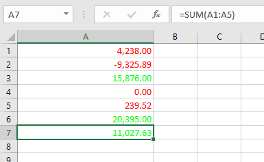
Numbers come in all kinds of formats in Excel worksheets. You may already be familiar with the pop-up window in Excel for making use of different numerical formats:
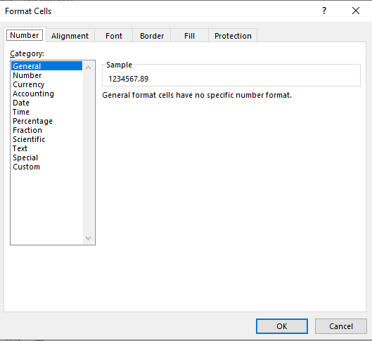
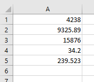
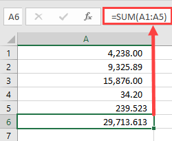
Formatting of numbers make the numbers easier to read and understand. The Excel default for numbers entered into cells is ‘General’ format, which means that the number is displayed exactly as you typed it in.
For example, if you enter a round number e.g. 4238, it will be displayed as 4238 with no decimal point or thousands separators. A decimal number such as 9325.89 will be displayed with the decimal point and the decimals. This means that it will not line up in the column with the round numbers, and will look extremely messy.
Also, without showing the thousands separators, it is difficult to see how large a number actually is without counting the individual digits. Is it in millions or tens of millions?
From the point of view of a user looking down a column of numbers, this makes it quite difficult to read and compare.
In VBA you have access to exactly the same range of formats that you have on the front end of Excel. This applies to not only an entered value in a cell on a worksheet, but also things like message boxes, UserForm controls, charts and graphs, and the Excel status bar at the bottom left hand corner of the worksheet.
The Format function is an extremely useful function in VBA in presentation terms, but it is also very complex in terms of the flexibility offered in how numbers are displayed.
How to Use the Format Function in VBA
If you are showing a message box, then the Format function can be used directly:
MsgBox Format(1234567.89, "#,##0.00")This will display a large number using commas to separate the thousands and to show 2 decimal places. The result will be 1,234,567.89. The zeros in place of the hash ensure that decimals will be shown as 00 in whole numbers, and that there is a leading zero for a number which is less than 1
The hashtag symbol (#) represents a digit placeholder which displays a digit if it is available in that position, or else nothing.
You can also use the format function to address an individual cell, or a range of cells to change the format:
Sheets("Sheet1").Range("A1:A10").NumberFormat = "#,##0.00"This code will set the range of cells (A1 to A10) to a custom format which separates the thousands with commas and shows 2 decimal places.
If you check the format of the cells on the Excel front end, you will find that a new custom format has been created.
You can also format numbers on the Excel Status Bar at the bottom left hand corner of the Excel window:
Application.StatusBar = Format(1234567.89, "#,##0.00")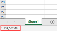
You clear this from the status bar by using:
Application.StatusBar = ""Creating a Format String
This example will add the text ‘Total Sales’ after each number, as well as including a thousands separator
Sheets("Sheet1").Range("A1:A6").NumberFormat = "#,##0.00"" Total Sales"""This is what your numbers will look like:
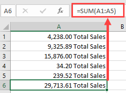
Note that cell A6 has a ‘SUM’ formula, and this will include the ‘Total Sales’ text without requiring formatting. If the formatting is applied, as in the above code, it will not put an extra instance of ‘Total Sales’ into cell A6
Although the cells now display alpha numeric characters, the numbers are still present in numeric form. The ‘SUM’ formula still works because it is using the numeric value in the background, not how the number is formatted.
The comma in the format string provides the thousands separator. Note that you only need to put this in the string once. If the number runs into millions or billions, it will still separate the digits into groups of 3
The zero in the format string (0) is a digit placeholder. It displays a digit if it is there, or a zero. Its positioning is very important to ensure uniformity with the formatting
In the format string, the hash characters (#) will display nothing if there is no digit. However, if there is a number like .8 (all decimals), we want it to show as 0.80 so that it lines up with the other numbers.
By using a single zero to the left of the decimal point and two zeros to the right of the decimal point in the format string, this will give the required result (0.80).
If there was only one zero to the right of the decimal point, then the result would be ‘0.8’ and everything would be displayed to one decimal place.
Using a Format String for Alignment
We may want to see all the decimal numbers in a range aligned on their decimal points, so that all the decimal points are directly under each other, however many places of decimals there are on each number.
You can use a question mark (?) within your format string to do this. The ‘?’ indicates that a number is shown if it is available, or a space
Sheets("Sheet1").Range("A1:A6").NumberFormat = "#,##0.00??"This will display your numbers as follows:
All the decimal points now line up underneath each other. Cell A5 has three decimal places and this would throw the alignment out normally, but using the ‘?’ character aligns everything perfectly.
Using Literal Characters Within the Format String
You can add any literal character into your format string by preceding it with a backslash ().
Suppose that you want to show a particular currency indicator for your numbers which is not based on your locale. The problem is that if you use a currency indicator, Excel automatically refers to your local and changes it to the one appropriate for the locale that is set on the Windows Control Panel. This could have implications if your Excel application is being distributed in other countries and you want to ensure that whatever the locale is, the currency indicator is always the same.
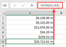
You may also want to indicate that the numbers are in millions in the following example:
Sheets("Sheet1").Range("A1:A6").NumberFormat = "$#,##0.00 m"This will produce the following results on your worksheet:
In using a backslash to display literal characters, you do not need to use a backslash for each individual character within a string. You can use:
Sheets("Sheet1").Range("A1:A6").NumberFormat = "$#,##0.00 mill"This will display ‘mill’ after every number within the formatted range.
You can use most characters as literals, but not reserved characters such as 0, #,?
Use of Commas in a Format String
We have already seen that commas can be used to create thousands separators for large numbers, but they can also be used in another way.
By using them at the end of the numeric part of the format string, they act as scalers of thousands. In other words, they will divide each number by 1,000 every time there is a comma.
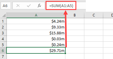
In the example data, we are showing it with an indicator that it is in millions. By inserting one comma into the format string, we can show those numbers divided by 1,000.
Sheets("Sheet1").Range("A1:A6").NumberFormat = "$#,##0.00,m"This will show the numbers divided by 1,000 although the original number will still be in background in the cell.
If you put two commas in the format string, then the numbers will be divided by a million
Sheets("Sheet1").Range("A1:A6").NumberFormat = "$#,##0.00,,m"This will be the result using only one comma (divide by 1,000):
VBA Coding Made Easy
Stop searching for VBA code online. Learn more about AutoMacro — A VBA Code Builder that allows beginners to code procedures from scratch with minimal coding knowledge and with many time-saving features for all users!

Learn More
Creating Conditional Formatting within the Format String
You could set up conditional formatting on the front end of Excel, but you can also do it within your VBA code, which means that you can manipulate the format string programmatically to make changes.
You can use up to four sections within your format string. Each section is delimited by a semicolon (;). The four sections correspond to positive, negative, zero, and text
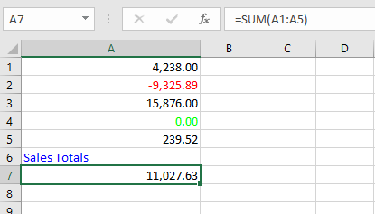
Range("A1:A7").NumberFormat = "#,##0.00;[Red]-#,##0.00;[Green] #,##0.00;[Blue]”In this example, we use the same hash, comma, and zero characters to provide thousand separators and two decimal points, but we now have different sections for each type of value.
The first section is for positive numbers and is no different to what we have already seen previously in terms of format.
The second section for negative numbers introduces a color (Red) which is held within a pair of square brackets. The format is the same as for positive numbers except that a minus (-) sign has been added in front.
The third section for zero numbers uses a color (Green) within square brackets with the numeric string the same as for positive numbers.
The final section is for text values, and all that this needs is a color (Blue) again within square brackets
This is the result of applying this format string:
You can go further with conditions within the format string. Suppose that you wanted to show every positive number above 10,000 as green, and every other number as red you could use this format string:
Range("A1:A7").NumberFormat = "[>=10000][Green]#,##0.00;[<10000][Red]#,##0.00"This format string includes conditions for >=10000 set in square brackets so that green will only be used where the number is greater than or equal to 10000
This is the result:
Using Fractions in Formatting Strings
Fractions are not often used in spreadsheets, since they normally equate to decimals which everyone is familiar with.
However, sometimes they do serve a purpose. This example will display dollars and cents:
Range("A1:A7").NumberFormat = "#,##0 "" dollars and "" 00/100 "" cents """This is the result that will be produced:
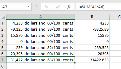
Remember that in spite of the numbers being displayed as text, they are still there in the background as numbers and all the Excel formulas can still be used on them.
Date and Time Formats
Dates are actually numbers and you can use formats on them in the same way as for numbers. If you format a date as a numeric number, you will see a large number to the left of the decimal point and a number of decimal places. The number to the left of the decimal point shows the number of days starting at 01-Jan-1900, and the decimal places show the time based on 24hrs
MsgBox Format(Now(), "dd-mmm-yyyy")This will format the current date to show ’08-Jul-2020’. Using ‘mmm’ for the month displays the first three characters of the month name. If you want the full month name then you use ‘mmmm’
You can include times in your format string:
MsgBox Format(Now(), "dd-mmm-yyyy hh:mm AM/PM")This will display ’08-Jul-2020 01:25 PM’
‘hh:mm’ represents hours and minutes and AM/PM uses a 12-hour clock as opposed to a 24-hour clock.
You can incorporate text characters into your format string:
MsgBox Format(Now(), "dd-mmm-yyyy hh:mm AM/PM"" today""")This will display ’08-Jul-2020 01:25 PM today’
You can also use literal characters using a backslash in front in the same way as for numeric format strings.
VBA Programming | Code Generator does work for you!
Predefined Formats
Excel has a number of built-in formats for both numbers and dates that you can use in your code. These mainly reflect what is available on the number formatting front end, although some of them go beyond what is normally available on the pop-up window. Also, you do not have the flexibility over number of decimal places, or whether thousands separators are used.
General Number
This format will display the number exactly as it is
MsgBox Format(1234567.89, "General Number")The result will be 1234567.89
Currency
MsgBox Format(1234567.894, "Currency")This format will add a currency symbol in front of the number e.g. $, £ depending on your locale, but it will also format the number to 2 decimal places and will separate the thousands with commas.
The result will be $1,234,567.89
Fixed
MsgBox Format(1234567.894, "Fixed")This format displays at least one digit to the left but only two digits to the right of the decimal point.
The result will be 1234567.89
Standard
MsgBox Format(1234567.894, "Standard")This displays the number with the thousand separators, but only to two decimal places.
The result will be 1,234,567.89
AutoMacro | Ultimate VBA Add-in | Click for Free Trial!
Percent
MsgBox Format(1234567.894, "Percent")The number is multiplied by 100 and a percentage symbol (%) is added at the end of the number. The format displays to 2 decimal places
The result will be 123456789.40%
Scientific
MsgBox Format(1234567.894, "Scientific")This converts the number to Exponential format
The result will be 1.23E+06
Yes/No
MsgBox Format(1234567.894, "Yes/No")This displays ‘No’ if the number is zero, otherwise displays ‘Yes’
The result will be ‘Yes’
True/False
MsgBox Format(1234567.894, "True/False")This displays ‘False’ if the number is zero, otherwise displays ‘True’
The result will be ‘True’
AutoMacro | Ultimate VBA Add-in | Click for Free Trial!
On/Off
MsgBox Format(1234567.894, "On/Off")This displays ‘Off’ if the number is zero, otherwise displays ‘On’
The result will be ‘On’
General Date
MsgBox Format(Now(), "General Date")This will display the date as date and time using AM/PM notation. How the date is displayed depends on your settings in the Windows Control Panel (Clock and Region | Region). It may be displayed as ‘mm/dd/yyyy’ or ‘dd/mm/yyyy’
The result will be ‘7/7/2020 3:48:25 PM’
Long Date
MsgBox Format(Now(), "Long Date")This will display a long date as defined in the Windows Control Panel (Clock and Region | Region). Note that it does not include the time.
The result will be ‘Tuesday, July 7, 2020’
Medium Date
MsgBox Format(Now(), "Medium Date")This displays a date as defined in the short date settings as defined by locale in the Windows Control Panel.
The result will be ’07-Jul-20’
AutoMacro | Ultimate VBA Add-in | Click for Free Trial!
Short Date
MsgBox Format(Now(), "Short Date")Displays a short date as defined in the Windows Control Panel (Clock and Region | Region). How the date is displayed depends on your locale. It may be displayed as ‘mm/dd/yyyy’ or ‘dd/mm/yyyy’
The result will be ‘7/7/2020’
Long Time
MsgBox Format(Now(), "Long Time")Displays a long time as defined in Windows Control Panel (Clock and Region | Region).
The result will be ‘4:11:39 PM’
Medium Time
MsgBox Format(Now(), "Medium Time")Displays a medium time as defined by your locale in the Windows Control Panel. This is usually set as 12-hour format using hours, minutes, and seconds and the AM/PM format.
The result will be ’04:15 PM’
Short Time
MsgBox Format(Now(), "Short Time")Displays a medium time as defined in Windows Control Panel (Clock and Region | Region). This is usually set as 24-hour format with hours and minutes
The result will be ’16:18’
AutoMacro | Ultimate VBA Add-in | Click for Free Trial!
Dangers of Using Excel’s Pre-Defined Formats in Dates and Times
The use of the pre-defined formats for dates and times in Excel VBA is very dependent on the settings in the Windows Control Panel and also what the locale is set to
Users can easily alter these settings, and this will have an effect on how your dates and times are displayed in Excel
For example, if you develop an Excel application which uses pre-defined formats within your VBA code, these may change completely if a user is in a different country or using a different locale to you. You may find that column widths do not fit the date definition, or on a user form the Active X control such as a combo box (drop down) control is too narrow for the dates and times to be displayed properly.
You need to consider where the audience is geographically when you develop your Excel application
User-Defined Formats for Numbers
There are a number of different parameters that you can use when defining your format string:
| Character | Description |
| Null String | No formatting |
| 0 | Digit placeholder. Displays a digit or a zero. If there is a digit for that position then it displays the digit otherwise it displays 0. If there are fewer digits than zeros, then you will get leading or trailing zeros. If there are more digits after the decimal point than there are zeros, then the number is rounded to the number of decimal places shown by the zeros. If there are more digits before the decimal point than zeros these will be displayed normally. |
| # | Digit placeholder. This displays a digit or nothing. It works the same as the zero placeholder above, except that leading and trailing zeros are not displayed. For example 0.75 would be displayed using zero placeholders, but this would be .75 using # placeholders. |
| . Decimal point. | Only one permitted per format string. This character depends on the settings in the Windows Control Panel. |
| % | Percentage placeholder. Multiplies number by 100 and places % character where it appears in the format string |
| , (comma) | Thousand separator. This is used if 0 or # placeholders are used and the format string contains a comma. One comma to the left of the decimal point indicates round to the nearest thousand. E.g. ##0, Two adjacent commas to the left of the thousand separator indicate rounding to the nearest million. E.g. ##0,, |
| E- E+ | Scientific format. This displays the number exponentially. |
| : (colon) | Time separator – used when formatting a time to split hours, minutes and seconds. |
| / | Date separator – this is used when specifying a format for a date |
| – + £ $ ( ) | Displays a literal character. To display a character other than listed here, precede it with a backslash () |
User-Defined Formats for Dates and Times
These characters can all be used in you format string when formatting dates and times:
| Character | Meaning |
| c | Displays the date as ddddd and the time as ttttt |
| d | Display the day as a number without leading zero |
| dd | Display the day as a number with leading zero |
| ddd | Display the day as an abbreviation (Sun – Sat) |
| dddd | Display the full name of the day (Sunday – Saturday) |
| ddddd | Display a date serial number as a complete date according to Short Date in the International settings of the windows Control Panel |
| dddddd | Displays a date serial number as a complete date according to Long Date in the International settings of the Windows Control Panel. |
| w | Displays the day of the week as a number (1 = Sunday) |
| ww | Displays the week of the year as a number (1-53) |
| m | Displays the month as a number without leading zero |
| mm | Displays the month as a number with leading zeros |
| mmm | Displays month as an abbreviation (Jan-Dec) |
| mmmm | Displays the full name of the month (January – December) |
| q | Displays the quarter of the year as a number (1-4) |
| y | Displays the day of the year as a number (1-366) |
| yy | Displays the year as a two-digit number |
| yyyy | Displays the year as four-digit number |
| h | Displays the hour as a number without leading zero |
| hh | Displays the hour as a number with leading zero |
| n | Displays the minute as a number without leading zero |
| nn | Displays the minute as a number with leading zero |
| s | Displays the second as a number without leading zero |
| ss | Displays the second as a number with leading zero |
| ttttt | Display a time serial number as a complete time. |
| AM/PM | Use a 12-hour clock and display AM or PM to indicate before or after noon. |
| am/pm | Use a 12-hour clock and use am or pm to indicate before or after noon |
| A/P | Use a 12-hour clock and use A or P to indicate before or after noon |
| a/p | Use a 12-hour clock and use a or p to indicate before or after noon |
“It is a capital mistake to theorize before one has data”- Sir Arthur Conan Doyle
This post covers everything you need to know about using Cells and Ranges in VBA. You can read it from start to finish as it is laid out in a logical order. If you prefer you can use the table of contents below to go to a section of your choice.
Topics covered include Offset property, reading values between cells, reading values to arrays and formatting cells.
A Quick Guide to Ranges and Cells
| Function | Takes | Returns | Example | Gives |
|---|---|---|---|---|
|
Range |
cell address | multiple cells | .Range(«A1:A4») | $A$1:$A$4 |
| Cells | row, column | one cell | .Cells(1,5) | $E$1 |
| Offset | row, column | multiple cells | Range(«A1:A2») .Offset(1,2) |
$C$2:$C$3 |
| Rows | row(s) | one or more rows | .Rows(4) .Rows(«2:4») |
$4:$4 $2:$4 |
| Columns | column(s) | one or more columns | .Columns(4) .Columns(«B:D») |
$D:$D $B:$D |
Download the Code
The Webinar
If you are a member of the VBA Vault, then click on the image below to access the webinar and the associated source code.
(Note: Website members have access to the full webinar archive.)

Introduction
This is the third post dealing with the three main elements of VBA. These three elements are the Workbooks, Worksheets and Ranges/Cells. Cells are by far the most important part of Excel. Almost everything you do in Excel starts and ends with Cells.
Generally speaking, you do three main things with Cells
- Read from a cell.
- Write to a cell.
- Change the format of a cell.
Excel has a number of methods for accessing cells such as Range, Cells and Offset.These can cause confusion as they do similar things and can lead to confusion
In this post I will tackle each one, explain why you need it and when you should use it.
Let’s start with the simplest method of accessing cells – using the Range property of the worksheet.
Important Notes
I have recently updated this article so that is uses Value2.
You may be wondering what is the difference between Value, Value2 and the default:
' Value2
Range("A1").Value2 = 56

' Value
Range("A1").Value = 56

' Default uses value
Range("A1") = 56
Using Value may truncate number if the cell is formatted as currency. If you don’t use any property then the default is Value.
It is better to use Value2 as it will always return the actual cell value(see this article from Charle Williams.)
The Range Property
The worksheet has a Range property which you can use to access cells in VBA. The Range property takes the same argument that most Excel Worksheet functions take e.g. “A1”, “A3:C6” etc.
The following example shows you how to place a value in a cell using the Range property.
' https://excelmacromastery.com/
Public Sub WriteToCell()

    ' Write number to cell A1 in sheet1 of this workbook
    ThisWorkbook.Worksheets("Sheet1").Range("A1").Value2 = 67

    ' Write text to cell A2 in sheet1 of this workbook
    ThisWorkbook.Worksheets("Sheet1").Range("A2").Value2 = "John Smith"

    ' Write date to cell A3 in sheet1 of this workbook
    ThisWorkbook.Worksheets("Sheet1").Range("A3").Value2 = #11/21/2017#

End Sub
As you can see Range is a member of the worksheet which in turn is a member of the Workbook. This follows the same hierarchy as in Excel so should be easy to understand. To do something with Range you must first specify the workbook and worksheet it belongs to.
For the rest of this post I will use the code name to reference the worksheet.

The following code shows the above example using the code name of the worksheet i.e. Sheet1 instead of ThisWorkbook.Worksheets(“Sheet1”).
' https://excelmacromastery.com/
Public Sub UsingCodeName()

    ' Write number to cell A1 in sheet1 of this workbook
    Sheet1.Range("A1").Value2 = 67

    ' Write text to cell A2 in sheet1 of this workbook
    Sheet1.Range("A2").Value2 = "John Smith"

    ' Write date to cell A3 in sheet1 of this workbook
    Sheet1.Range("A3").Value2 = #11/21/2017#

End Sub
You can also write to multiple cells using the Range property
' https://excelmacromastery.com/
Public Sub WriteToMulti()

    ' Write number to a range of cells
    Sheet1.Range("A1:A10").Value2 = 67

    ' Write text to multiple ranges of cells
    Sheet1.Range("B2:B5,B7:B9").Value2 = "John Smith"

End Sub
You can download working examples of all the code from this post from the top of this article.
The Cells Property of the Worksheet
The worksheet object has another property called Cells which is very similar to range. There are two differences
- Cells returns a range of one cell only.
- Cells takes row and column as arguments.
The example below shows you how to write values to cells using both the Range and Cells property
' https://excelmacromastery.com/
Public Sub UsingCells()

    ' Write to A1
    Sheet1.Range("A1").Value2 = 10
    Sheet1.Cells(1, 1).Value2  = 10

    ' Write to A10
    Sheet1.Range("A10").Value2 = 10
    Sheet1.Cells(10, 1).Value2  = 10

    ' Write to E1
    Sheet1.Range("E1").Value2 = 10
    Sheet1.Cells(1, 5).Value2  = 10

End Sub
You may be wondering when you should use Cells and when you should use Range. Using Range is useful for accessing the same cells each time the Macro runs.
For example, if you were using a Macro to calculate a total and write it to cell A10 every time then Range would be suitable for this task.
Using the Cells property is useful if you are accessing a cell based on a number that may vary. It is easier to explain this with an example.
In the following code, we ask the user to specify the column number. Using Cells gives us the flexibility to use a variable number for the column.
' https://excelmacromastery.com/
Public Sub WriteToColumn()

    Dim UserCol As Integer

    ' Get the column number from the user
    UserCol = Application.InputBox(" Please enter the column...", Type:=1)

    ' Write text to user selected column
    Sheet1.Cells(1, UserCol).Value2 = "John Smith"

End Sub
In the above example, we are using a number for the column rather than a letter.
To use Range here would require us to convert these values to the letter/number cell reference e.g. “C1”. Using the Cells property allows us to provide a row and a column number to access a cell.
Sometimes you may want to return more than one cell using row and column numbers. The next section shows you how to do this.
Using Cells and Range together
As you have seen you can only access one cell using the Cells property. If you want to return a range of cells then you can use Cells with Ranges as follows
' https://excelmacromastery.com/
Public Sub UsingCellsWithRange()

    With Sheet1
        ' Write 5 to Range A1:A10 using Cells property
        .Range(.Cells(1, 1), .Cells(10, 1)).Value2 = 5

        ' Format Range B1:Z1 to be bold
        .Range(.Cells(1, 2), .Cells(1, 26)).Font.Bold = True

    End With

End Sub
As you can see, you provide the start and end cell of the Range. Sometimes it can be tricky to see which range you are dealing with when the value are all numbers. Range has a property called Address which displays the letter/ number cell reference of any range. This can come in very handy when you are debugging or writing code for the first time.
In the following example we print out the address of the ranges we are using:
' https://excelmacromastery.com/
Public Sub ShowRangeAddress()

    ' Note: Using underscore allows you to split up lines of code
    With Sheet1

        ' Write 5 to Range A1:A10 using Cells property
        .Range(.Cells(1, 1), .Cells(10, 1)).Value2 = 5
        Debug.Print "First address is : " _
            + .Range(.Cells(1, 1), .Cells(10, 1)).Address

        ' Format Range B1:Z1 to be bold
        .Range(.Cells(1, 2), .Cells(1, 26)).Font.Bold = True
        Debug.Print "Second address is : " _
            + .Range(.Cells(1, 2), .Cells(1, 26)).Address

    End With

End Sub
In the example I used Debug.Print to print to the Immediate Window. To view this window select View->Immediate Window(or Ctrl G)


You can download all the code for this post from the top of this article.
The Offset Property of Range
Range has a property called Offset. The term Offset refers to a count from the original position. It is used a lot in certain areas of programming. With the Offset property you can get a Range of cells the same size and a certain distance from the current range. The reason this is useful is that sometimes you may want to select a Range based on a certain condition. For example in the screenshot below there is a column for each day of the week. Given the day number(i.e. Monday=1, Tuesday=2 etc.) we need to write the value to the correct column.

We will first attempt to do this without using Offset.
' https://excelmacromastery.com/
' This sub tests with different values
Public Sub TestSelect()

    ' Monday
    SetValueSelect 1, 111.21
    ' Wednesday
    SetValueSelect 3, 456.99
    ' Friday
    SetValueSelect 5, 432.25
    ' Sunday
    SetValueSelect 7, 710.17

End Sub

' Writes the value to a column based on the day
Public Sub SetValueSelect(lDay As Long, lValue As Currency)

    Select Case lDay
        Case 1: Sheet1.Range("H3").Value2 = lValue
        Case 2: Sheet1.Range("I3").Value2 = lValue
        Case 3: Sheet1.Range("J3").Value2 = lValue
        Case 4: Sheet1.Range("K3").Value2 = lValue
        Case 5: Sheet1.Range("L3").Value2 = lValue
        Case 6: Sheet1.Range("M3").Value2 = lValue
        Case 7: Sheet1.Range("N3").Value2 = lValue
    End Select

End Sub
As you can see in the example, we need to add a line for each possible option. This is not an ideal situation. Using the Offset Property provides a much cleaner solution
' https://excelmacromastery.com/
' This sub tests with different values
Public Sub TestOffset()

    DayOffSet 1, 111.01
    DayOffSet 3, 456.99
    DayOffSet 5, 432.25
    DayOffSet 7, 710.17

End Sub

Public Sub DayOffSet(lDay As Long, lValue As Currency)

    ' We use the day value with offset specify the correct column
    Sheet1.Range("G3").Offset(, lDay).Value2 = lValue

End Sub
As you can see this solution is much better. If the number of days in increased then we do not need to add any more code. For Offset to be useful there needs to be some kind of relationship between the positions of the cells. If the Day columns in the above example were random then we could not use Offset. We would have to use the first solution.
One thing to keep in mind is that Offset retains the size of the range. So .Range(“A1:A3”).Offset(1,1) returns the range B2:B4. Below are some more examples of using Offset
' https://excelmacromastery.com/
Public Sub UsingOffset()

    ' Write to B2 - no offset
    Sheet1.Range("B2").Offset().Value2 = "Cell B2"

    ' Write to C2 - 1 column to the right
    Sheet1.Range("B2").Offset(, 1).Value2 = "Cell C2"

    ' Write to B3 - 1 row down
    Sheet1.Range("B2").Offset(1).Value2 = "Cell B3"

    ' Write to C3 - 1 column right and 1 row down
    Sheet1.Range("B2").Offset(1, 1).Value2 = "Cell C3"

    ' Write to A1 - 1 column left and 1 row up
    Sheet1.Range("B2").Offset(-1, -1).Value2 = "Cell A1"

    ' Write to range E3:G13 - 1 column right and 1 row down
    Sheet1.Range("D2:F12").Offset(1, 1).Value2 = "Cells E3:G13"

End Sub
Using the Range CurrentRegion
CurrentRegion returns a range of all the adjacent cells to the given range.
In the screenshot below you can see the two current regions. I have added borders to make the current regions clear.

A row or column of blank cells signifies the end of a current region.
You can manually check the CurrentRegion in Excel by selecting a range and pressing Ctrl + Shift + *.
If we take any range of cells within the border and apply CurrentRegion, we will get back the range of cells in the entire area.
For example
Range(“B3”).CurrentRegion will return the range B3:D14
Range(“D14”).CurrentRegion will return the range B3:D14
Range(“C8:C9”).CurrentRegion will return the range B3:D14
and so on
How to Use
We get the CurrentRegion as follows
' Current region will return B3:D14 from above example
Dim rg As Range
Set rg = Sheet1.Range("B3").CurrentRegion
Read Data Rows Only
Read through the range from the second row i.e.skipping the header row
' Current region will return B3:D14 from above example
Dim rg As Range
Set rg = Sheet1.Range("B3").CurrentRegion

' Start at row 2 - row after header
Dim i As Long
For i = 2 To rg.Rows.Count
    ' current row, column 1 of range
    Debug.Print rg.Cells(i, 1).Value2
Next i
Remove Header
Remove header row(i.e. first row) from the range. For example if range is A1:D4 this will return A2:D4
' Current region will return B3:D14 from above example
Dim rg As Range
Set rg = Sheet1.Range("B3").CurrentRegion

' Remove Header
Set rg = rg.Resize(rg.Rows.Count - 1).Offset(1)

' Start at row 1 as no header row
Dim i As Long
For i = 1 To rg.Rows.Count
    ' current row, column 1 of range
    Debug.Print rg.Cells(i, 1).Value2
Next i
Using Rows and Columns as Ranges
If you want to do something with an entire Row or Column you can use the Rows or Columns property of the Worksheet. They both take one parameter which is the row or column number you wish to access
' https://excelmacromastery.com/
Public Sub UseRowAndColumns()

    ' Set the font size of column B to 9
    Sheet1.Columns(2).Font.Size = 9

    ' Set the width of columns D to F
    Sheet1.Columns("D:F").ColumnWidth = 4

    ' Set the font size of row 5 to 18
    Sheet1.Rows(5).Font.Size = 18

End Sub
Using Range in place of Worksheet
You can also use Cells, Rows and Columns as part of a Range rather than part of a Worksheet. You may have a specific need to do this but otherwise I would avoid the practice. It makes the code more complex. Simple code is your friend. It reduces the possibility of errors.
The code below will set the second column of the range to bold. As the range has only two rows the entire column is considered B1:B2
' https://excelmacromastery.com/
Public Sub UseColumnsInRange()

    ' This will set B1 and B2 to be bold
    Sheet1.Range("A1:C2").Columns(2).Font.Bold = True

End Sub
You can download all the code for this post from the top of this article.
Reading Values from one Cell to another
In most of the examples so far we have written values to a cell. We do this by placing the range on the left of the equals sign and the value to place in the cell on the right. To write data from one cell to another we do the same. The destination range goes on the left and the source range goes on the right.
The following example shows you how to do this:
' https://excelmacromastery.com/
Public Sub ReadValues()

    ' Place value from B1 in A1
    Sheet1.Range("A1").Value2 = Sheet1.Range("B1").Value2

    ' Place value from B3 in sheet2 to cell A1
    Sheet1.Range("A1").Value2 = Sheet2.Range("B3").Value2

    ' Place value from B1 in cells A1 to A5
    Sheet1.Range("A1:A5").Value2 = Sheet1.Range("B1").Value2

    ' You need to use the "Value" property to read multiple cells
    Sheet1.Range("A1:A5").Value2 = Sheet1.Range("B1:B5").Value2

End Sub
As you can see from this example it is not possible to read from multiple cells. If you want to do this you can use the Copy function of Range with the Destination parameter
' https://excelmacromastery.com/
Public Sub CopyValues()

    ' Store the copy range in a variable
    Dim rgCopy As Range
    Set rgCopy = Sheet1.Range("B1:B5")

    ' Use this to copy from more than one cell
    rgCopy.Copy Destination:=Sheet1.Range("A1:A5")

    ' You can paste to multiple destinations
    rgCopy.Copy Destination:=Sheet1.Range("A1:A5,C2:C6")

End Sub
The Copy function copies everything including the format of the cells. It is the same result as manually copying and pasting a selection. You can see more about it in the Copying and Pasting Cells section.
Using the Range.Resize Method
When copying from one range to another using assignment(i.e. the equals sign), the destination range must be the same size as the source range.
Using the Resize function allows us to resize a range to a given number of rows and columns.
For example:
' https://excelmacromastery.com/
Sub ResizeExamples()

    ' Prints A1
    Debug.Print Sheet1.Range("A1").Address

    ' Prints A1:A2
    Debug.Print Sheet1.Range("A1").Resize(2, 1).Address

    ' Prints A1:A5
    Debug.Print Sheet1.Range("A1").Resize(5, 1).Address

    ' Prints A1:D1
    Debug.Print Sheet1.Range("A1").Resize(1, 4).Address

    ' Prints A1:C3
    Debug.Print Sheet1.Range("A1").Resize(3, 3).Address

End Sub
When we want to resize our destination range we can simply use the source range size.
In other words, we use the row and column count of the source range as the parameters for resizing:
' https://excelmacromastery.com/
Sub Resize()

    Dim rgSrc As Range, rgDest As Range

    ' Get all the data in the current region
    Set rgSrc = Sheet1.Range("A1").CurrentRegion

      ' Get the range destination
    Set rgDest = Sheet2.Range("A1")
    Set rgDest = rgDest.Resize(rgSrc.Rows.Count, rgSrc.Columns.Count)

    rgDest.Value2 = rgSrc.Value2

End Sub
We can do the resize in one line if we prefer:
' https://excelmacromastery.com/
Sub ResizeOneLine()

    Dim rgSrc As Range

    ' Get all the data in the current region
    Set rgSrc = Sheet1.Range("A1").CurrentRegion

    With rgSrc
        Sheet2.Range("A1").Resize(.Rows.Count, .Columns.Count).Value2 = .Value2
    End With

End Sub
Reading Values to variables
We looked at how to read from one cell to another. You can also read from a cell to a variable. A variable is used to store values while a Macro is running. You normally do this when you want to manipulate the data before writing it somewhere. The following is a simple example using a variable. As you can see the value of the item to the right of the equals is written to the item to the left of the equals.
' https://excelmacromastery.com/
Public Sub UseVariables()

    ' Create
    Dim number As Long

    ' Read number from cell
    number = Sheet1.Range("A1").Value2

    ' Add 1 to value
    number = number + 1

    ' Write new value to cell
    Sheet1.Range("A2").Value2 = number

End Sub
To read text to a variable you use a variable of type String:
' https://excelmacromastery.com/
Public Sub UseVariableText()

    ' Declare a variable of type string
    Dim text As String

    ' Read value from cell
    text = Sheet1.Range("A1").Value2

    ' Write value to cell
    Sheet1.Range("A2").Value2 = text

End Sub
You can write a variable to a range of cells. You just specify the range on the left and the value will be written to all cells in the range.
' https://excelmacromastery.com/
Public Sub VarToMulti()

    ' Read value from cell
    Sheet1.Range("A1:B10").Value2 = 66

End Sub
You cannot read from multiple cells to a variable. However you can read to an array which is a collection of variables. We will look at doing this in the next section.
How to Copy and Paste Cells
If you want to copy and paste a range of cells then you do not need to select them. This is a common error made by new VBA users.
Note: We normally use Range.Copy when we want to copy formats, formulas, validation. If we want to copy values it is not the most efficient method.
I have written a complete guide to copying data in Excel VBA here.
You can simply copy a range of cells like this:
Range("A1:B4").Copy Destination:=Range("C5")
Using this method copies everything – values, formats, formulas and so on. If you want to copy individual items you can use the PasteSpecial property of range.
It works like this
Range("A1:B4").Copy
Range("F3").PasteSpecial Paste:=xlPasteValues
Range("F3").PasteSpecial Paste:=xlPasteFormats
Range("F3").PasteSpecial Paste:=xlPasteFormulas
The following table shows a full list of all the paste types
| Paste Type |
|---|
| xlPasteAll |
| xlPasteAllExceptBorders |
| xlPasteAllMergingConditionalFormats |
| xlPasteAllUsingSourceTheme |
| xlPasteColumnWidths |
| xlPasteComments |
| xlPasteFormats |
| xlPasteFormulas |
| xlPasteFormulasAndNumberFormats |
| xlPasteValidation |
| xlPasteValues |
| xlPasteValuesAndNumberFormats |
Reading a Range of Cells to an Array
You can also copy values by assigning the value of one range to another.
Range("A3:Z3").Value2 = Range("A1:Z1").Value2
The value of range in this example is considered to be a variant array. What this means is that you can easily read from a range of cells to an array. You can also write from an array to a range of cells. If you are not familiar with arrays you can check them out in this post.
The following code shows an example of using an array with a range:
' https://excelmacromastery.com/
Public Sub ReadToArray()

    ' Create dynamic array
    Dim StudentMarks() As Variant

    ' Read 26 values into array from the first row
    StudentMarks = Range("A1:Z1").Value2

    ' Do something with array here

    ' Write the 26 values to the third row
    Range("A3:Z3").Value2 = StudentMarks

End Sub
Keep in mind that the array created by the read is a 2 dimensional array. This is because a spreadsheet stores values in two dimensions i.e. rows and columns
Going through all the cells in a Range
Sometimes you may want to go through each cell one at a time to check value.
You can do this using a For Each loop shown in the following code
' https://excelmacromastery.com/
Public Sub TraversingCells()

    ' Go through each cells in the range
    Dim rg As Range
    For Each rg In Sheet1.Range("A1:A10,A20")
        ' Print address of cells that are negative
        If rg.Value < 0 Then
            Debug.Print rg.Address + " is negative."
        End If
    Next

End Sub
You can also go through consecutive Cells using the Cells property and a standard For loop.
The standard loop is more flexible about the order you use but it is slower than a For Each loop.
' https://excelmacromastery.com/
Public Sub TraverseCells()

    ' Go through cells from A1 to A10
    Dim i As Long
    For i = 1 To 10
        ' Print address of cells that are negative
        If Range("A" & i).Value < 0 Then
            Debug.Print Range("A" & i).Address + " is negative."
        End If
    Next

    ' Go through cells in reverse i.e. from A10 to A1
    For i = 10 To 1 Step -1
        ' Print address of cells that are negative
        If Range("A" & i) < 0 Then
            Debug.Print Range("A" & i).Address + " is negative."
        End If
    Next

End Sub
Formatting Cells
Sometimes you will need to format the cells the in spreadsheet. This is actually very straightforward. The following example shows you various formatting you can add to any range of cells
' https://excelmacromastery.com/
Public Sub FormattingCells()

    With Sheet1

        ' Format the font
        .Range("A1").Font.Bold = True
        .Range("A1").Font.Underline = True
        .Range("A1").Font.Color = rgbNavy

        ' Set the number format to 2 decimal places
        .Range("B2").NumberFormat = "0.00"
        ' Set the number format to a date
        .Range("C2").NumberFormat = "dd/mm/yyyy"
        ' Set the number format to general
        .Range("C3").NumberFormat = "General"
        ' Set the number format to text
        .Range("C4").NumberFormat = "Text"

        ' Set the fill color of the cell
        .Range("B3").Interior.Color = rgbSandyBrown

        ' Format the borders
        .Range("B4").Borders.LineStyle = xlDash
        .Range("B4").Borders.Color = rgbBlueViolet

    End With

End Sub
Main Points
The following is a summary of the main points
- Range returns a range of cells
- Cells returns one cells only
- You can read from one cell to another
- You can read from a range of cells to another range of cells.
- You can read values from cells to variables and vice versa.
- You can read values from ranges to arrays and vice versa
- You can use a For Each or For loop to run through every cell in a range.
- The properties Rows and Columns allow you to access a range of cells of these types
What’s Next?
Free VBA Tutorial If you are new to VBA or you want to sharpen your existing VBA skills then why not try out the The Ultimate VBA Tutorial.
Related Training: Get full access to the Excel VBA training webinars and all the tutorials.
(NOTE: Planning to build or manage a VBA Application? Learn how to build 10 Excel VBA applications from scratch.)