Vba excel format column

You probably already know that VBA (Visual Basic for Applications) is an amazing tool to use to automate processes in Excel. It is also a great tool to help potential users do various things.

In the example below, we will present how to format any given column as text with the help of VBA.

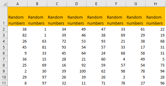
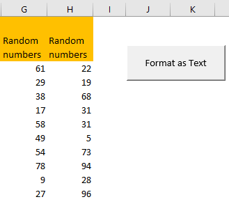
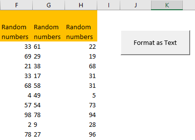
For our example, we will input random numbers from 1 to 100 in range A2:H11:

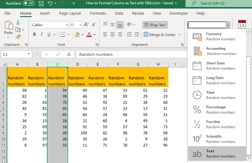
To format any of these columns as Text manually, we need to select any column (for example column C), then go to the Home tab and in Numbers sub-section choose Text on a dropdown:

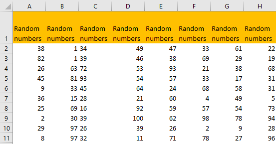
Now our table with random numbers looks like this:

Let us now try to do these steps, but by using VBA. First thing first, we need to access the module by clicking the combination of ALT + F11.

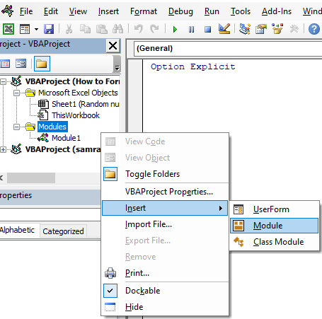
Once in the module, we will right-click on it and choose Insert >> Module:

When we click on it, we will input the following code on the right side of our screen:

Sub FormatAsText()     Dim col As String     col = InputBox(PROMPT:=«Which column Do you want To convert To text?»)     Columns(col).Select     Selection.NumberFormat = «@» End Sub

This is what our code looks like in the module:

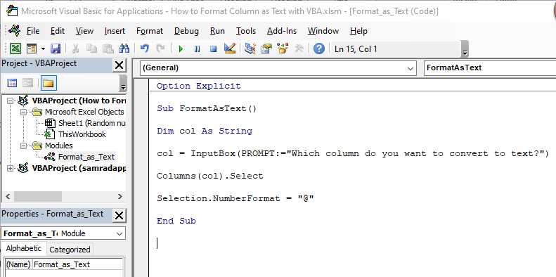
What our code does is it first creates a “col” variable and then declares that variable to be equal to the answer or the user on the question below:

Dim col As String col = InputBox(PROMPT:=«Which column do you want to convert to text?»)

Then we select the column that the user wanted to change and change the format of that selection (that column) to text.

Columns(col).Select Selection.NumberFormat = «@»

Now, our code has a significant error, and that is it will simply fail if the user clicks something other than an actual column name, but for the sake of this exercise, we will presume that our user knows what we are talking about.

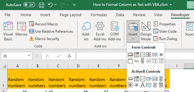
We will now add our code to our sheet by going to it, and then going to Developer tab >> Controls >> Insert >> Form Controls >> Button (first option available):

We will then insert the button next to our table. As soon as we set the destination, we will be presented with the following window:

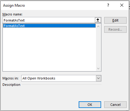
We will assign our existing macro (FormatAsText) to our button, which means that we will be able to run our macro by clicking on our button.

We will change the name of our button to “Format as Text”.

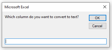
Now, when we click on this button, our code will be executed. The first thing that the user will see is the pop-up window with the question we defined:

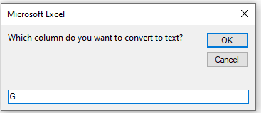
We will choose column G, for the sake of the exercise.

When we click OK, we will see that our column G has been formatted:

Post Views: 2,449

Formatting Cells Number

General

Range("A1").NumberFormat = "General"

Number

Range("A1").NumberFormat = "0.00"

Currency

Range("A1").NumberFormat = "$#,##0.00"

Accounting

Range("A1").NumberFormat = "_($* #,##0.00_);_($* (#,##0.00);_($* ""-""??_);_(@_)"

Date

Range("A1").NumberFormat = "yyyy-mm-dd;@"

Time

Range("A1").NumberFormat = "h:mm:ss AM/PM;@"

Percentage

Range("A1").NumberFormat = "0.00%"

Fraction

Range("A1").NumberFormat = "# ?/?"

Scientific

Range("A1").NumberFormat = "0.00E+00"

Text

Range("A1").NumberFormat = "@"

Special

Range("A1").NumberFormat = "00000"

Custom

Range("A1").NumberFormat = "$#,##0.00_);[Red]($#,##0.00)"

Formatting Cells Alignment

Text Alignment

Horizontal

The value of this property can be set to one of the constants: xlGeneral, xlCenter, xlDistributed, xlJustify, xlLeft, xlRight.

The following code sets the horizontal alignment of cell A1 to center.

Range("A1").HorizontalAlignment = xlCenter

Vertical

The value of this property can be set to one of the constants: xlBottom, xlCenter, xlDistributed, xlJustify, xlTop.

The following code sets the vertical alignment of cell A1 to bottom.

Range("A1").VerticalAlignment = xlBottom

Text Control

Wrap Text

This example formats cell A1 so that the text wraps within the cell.

Range("A1").WrapText = True

Shrink To Fit

This example causes text in row one to automatically shrink to fit in the available column width.

Rows(1).ShrinkToFit = True

Merge Cells

This example merge range A1:A4 to a large one.

Range("A1:A4").MergeCells = True

Right-to-left

Text direction

The value of this property can be set to one of the constants: xlRTL (right-to-left), xlLTR (left-to-right), or xlContext (context).

The following code example sets the reading order of cell A1 to xlRTL (right-to-left).

Range("A1").ReadingOrder = xlRTL

Orientation

The value of this property can be set to an integer value from –90 to 90 degrees or to one of the following constants: xlDownward, xlHorizontal, xlUpward, xlVertical.

The following code example sets the orientation of cell A1 to xlHorizontal.

Range("A1").Orientation = xlHorizontal

Font

Font Name

The value of this property can be set to one of the fonts: Calibri, Times new Roman, Arial…

The following code sets the font name of range A1:A5 to Calibri.

Range("A1:A5").Font.Name = "Calibri"

Font Style

The value of this property can be set to one of the constants: Regular, Bold, Italic, Bold Italic.

The following code sets the font style of range A1:A5 to Italic.

Range("A1:A5").Font.FontStyle = "Italic"

Font Size

The value of this property can be set to an integer value from 1 to 409.

The following code sets the font size of cell A1 to 14.

Range("A1").Font.Size = 14

Underline

The value of this property can be set to one of the constants: xlUnderlineStyleNone, xlUnderlineStyleSingle, xlUnderlineStyleDouble, xlUnderlineStyleSingleAccounting, xlUnderlineStyleDoubleAccounting.

The following code sets the font of cell A1 to xlUnderlineStyleDouble (double underline).

Range("A1").Font.Underline = xlUnderlineStyleDouble

Font Color

The value of this property can be set to one of the standard colors: vbBlack, vbRed, vbGreen, vbYellow, vbBlue, vbMagenta, vbCyan, vbWhite or an integer value from 0 to 16,581,375.

To assist you with specifying the color of anything, the VBA is equipped with a function named RGB. Its syntax is:

Function RGB(RedValue As Byte, GreenValue As Byte, BlueValue As Byte) As long

This function takes three arguments and each must hold a value between 0 and 255. The first argument represents the ratio of red of the color. The second argument represents the green ratio of the color. The last argument represents the blue of the color. After the function has been called, it produces a number whose maximum value can be 255 * 255 * 255 = 16,581,375, which represents a color.

The following code sets the font color of cell A1 to vbBlack (Black).

Range("A1").Font.Color = vbBlack

The following code sets the font color of cell A1 to 0 (Black).

Range("A1").Font.Color = 0

The following code sets the font color of cell A1 to RGB(0, 0, 0) (Black).

Range("A1").Font.Color = RGB(0, 0, 0)

Font Effects

Strikethrough

True if the font is struck through with a horizontal line.

The following code sets the font of cell A1 to strikethrough.

Range("A1").Font.Strikethrough = True

Subscript

True if the font is formatted as subscript. False by default.

The following code sets the font of cell A1 to Subscript.

Range("A1").Font.Subscript = True

Superscript

True if the font is formatted as superscript; False by default.

The following code sets the font of cell A1 to Superscript.

Range("A1").Font.Superscript = True

Border

Border Index

Using VBA you can choose to create borders for the different edges of a range of cells:

1. xlDiagonalDown (Border running from the upper left-hand corner to the lower right of each cell in the range).
2. xlDiagonalUp (Border running from the lower left-hand corner to the upper right of each cell in the range).
3. xlEdgeBottom (Border at the bottom of the range).
4. xlEdgeLeft (Border at the left-hand edge of the range).
5. xlEdgeRight (Border at the right-hand edge of the range).
6. xlEdgeTop (Border at the top of the range).
7. xlInsideHorizontal (Horizontal borders for all cells in the range except borders on the outside of the range).
8. xlInsideVertical (Vertical borders for all the cells in the range except borders on the outside of the range).

Line Style

The value of this property can be set to one of the constants: xlContinuous (Continuous line), xlDash (Dashed line), xlDashDot (Alternating dashes and dots), xlDashDotDot (Dash followed by two dots), xlDot (Dotted line), xlDouble (Double line), xlLineStyleNone (No line), xlSlantDashDot (Slanted dashes).

The following code example sets the border on the bottom edge of cell A1 with continuous line.

Range("A1").Borders(xlEdgeBottom).LineStyle = xlContinuous

The following code example removes the border on the bottom edge of cell A1.

Range("A1").Borders(xlEdgeBottom).LineStyle = xlNone

Line Thickness

The value of this property can be set to one of the constants: xlHairline (Hairline, thinnest border), xlMedium (Medium), xlThick (Thick, widest border), xlThin (Thin).

The following code example sets the thickness of the border created to xlThin (Thin).

Range("A1").Borders(xlEdgeBottom).Weight = xlThin

Line Color

The value of this property can be set to one of the standard colors: vbBlack, vbRed, vbGreen, vbYellow, vbBlue, vbMagenta, vbCyan, vbWhite or an integer value from 0 to 16,581,375.

The following code example sets the color of the border on the bottom edge to green.

Range("A1").Borders(xlEdgeBottom).Color = vbGreen

You can also use the RGB function to create a color value.

The following example sets the color of the bottom border of cell A1 with RGB fuction.

Range("A1").Borders(xlEdgeBottom).Color = RGB(255, 0, 0)

Fill

Pattern Style

The value of this property can be set to one of the constants:

1. xlPatternAutomatic (Excel controls the pattern.)
2. xlPatternChecker (Checkerboard.)
3. xlPatternCrissCross (Criss-cross lines.)
4. xlPatternDown (Dark diagonal lines running from the upper left to the lower right.)
5. xlPatternGray16 (16% gray.)
6. xlPatternGray25 (25% gray.)
7. xlPatternGray50 (50% gray.)
8. xlPatternGray75 (75% gray.)
9. xlPatternGray8 (8% gray.)
10. xlPatternGrid (Grid.)
11. xlPatternHorizontal (Dark horizontal lines.)
12. xlPatternLightDown (Light diagonal lines running from the upper left to the lower right.)
13. xlPatternLightHorizontal (Light horizontal lines.)
14. xlPatternLightUp (Light diagonal lines running from the lower left to the upper right.)
15. xlPatternLightVertical (Light vertical bars.)
16. xlPatternNone (No pattern.)
17. xlPatternSemiGray75 (75% dark moiré.)
18. xlPatternSolid (Solid color.)
19. xlPatternUp (Dark diagonal lines running from the lower left to the upper right.)

Protection

Locking Cells

This property returns True if the object is locked, False if the object can be modified when the sheet is protected, or Null if the specified range contains both locked and unlocked cells.

The following code example unlocks cells A1:B22 on Sheet1 so that they can be modified when the sheet is protected.

Worksheets("Sheet1").Range("A1:B22").Locked = False
Worksheets("Sheet1").Protect

Hiding Formulas

This property returns True if the formula will be hidden when the worksheet is protected, Null if the specified range contains some cells with FormulaHidden equal to True and some cells with FormulaHidden equal to False.

Don’t confuse this property with the Hidden property. The formula will not be hidden if the workbook is protected and the worksheet is not, but only if the worksheet is protected.

The following code example hides the formulas in cells A1 and C1 on Sheet1 when the worksheet is protected.

Worksheets("Sheet1").Range("A1:C1").FormulaHidden = True

Formatting Numbers in Excel VBA

Numbers come in all kinds of formats in Excel worksheets. You may already be familiar with the pop-up window in Excel for making use of different numerical formats:

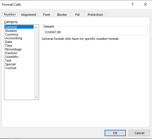
Formatting of numbers make the numbers easier to read and understand. The Excel default for numbers entered into cells is ‘General’ format, which means that the number is displayed exactly as you typed it in.

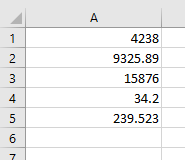
For example, if you enter a round number e.g. 4238, it will be displayed as 4238 with no decimal point or thousands separators. A decimal number such as 9325.89 will be displayed with the decimal point and the decimals. This means that it will not line up in the column with the round numbers, and will look extremely messy.

Also, without showing the thousands separators, it is difficult to see how large a number actually is without counting the individual digits.  Is it in millions or tens of millions?

From the point of view of a user looking down a column of numbers, this makes it quite difficult to read and compare.

In VBA you have access to exactly the same range of formats that you have on the front end of Excel. This applies to not only an entered value in a cell on a worksheet, but also things like message boxes, UserForm controls, charts and graphs, and the Excel status bar at the bottom left hand corner of the worksheet.

The Format function is an extremely useful function in VBA in presentation terms, but it is also very complex in terms of the flexibility offered in how numbers are displayed.

How to Use the Format Function in VBA

If you are showing a message box, then the Format function can be used directly:

MsgBox Format(1234567.89, "#,##0.00")

This will display a large number using commas to separate the thousands and to show 2 decimal places.  The result will be 1,234,567.89.  The zeros in place of the hash ensure that decimals will be shown as 00 in whole numbers, and that there is a leading zero for a number which is less than 1

The hashtag symbol (#) represents a digit placeholder which displays a digit if it is available in that position, or else nothing.

You can also use the format function to address an individual cell, or a range of cells to change the format:

Sheets("Sheet1").Range("A1:A10").NumberFormat = "#,##0.00"

This code will set the range of cells (A1 to A10) to a custom format which separates the thousands with commas and shows 2 decimal places.

If you check the format of the cells on the Excel front end, you will find that a new custom format has been created.

You can also format numbers on the Excel Status Bar at the bottom left hand corner of the Excel window:

Application.StatusBar = Format(1234567.89, "#,##0.00")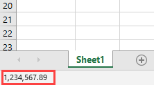

You clear this from the status bar by using:

Application.StatusBar = ""

Creating a Format String

This example will add the text ‘Total Sales’ after each number, as well as including a thousands separator

Sheets("Sheet1").Range("A1:A6").NumberFormat = "#,##0.00"" Total Sales"""

This is what your numbers will look like:

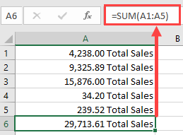
Note that cell A6 has a ‘SUM’ formula, and this will include the ‘Total Sales’ text without requiring formatting.  If the formatting is applied, as in the above code, it will not put an extra instance of ‘Total Sales’ into cell A6

Although the cells now display alpha numeric characters, the numbers are still present in numeric form. The ‘SUM’ formula still works because it is using the numeric value in the background, not how the number is formatted.

The comma in the format string provides the thousands separator. Note that you only need to put this in the string once.  If the number runs into millions or billions, it will still separate the digits into groups of 3

The zero in the format string (0) is a digit placeholder. It displays a digit if it is there, or a zero. Its positioning is very important to ensure uniformity with the formatting

In the format string, the hash characters (#) will display nothing if there is no digit.  However, if there is a number like .8 (all decimals), we want it to show as 0.80 so that it lines up with the other numbers.

By using a single zero to the left of the decimal point and two zeros to the right of the decimal point in the format string, this will give the required result (0.80).

If there was only one zero to the right of the decimal point, then the result would be ‘0.8’ and everything would be displayed to one decimal place.

Using a Format String for Alignment

We may want to see all the decimal numbers in a range aligned on their decimal points, so that all the decimal points are directly under each other, however many places of decimals there are on each number.

You can use a question mark (?) within your format string to do this.  The ‘?’ indicates that a number is shown if it is available, or a space

Sheets("Sheet1").Range("A1:A6").NumberFormat = "#,##0.00??"

This will display your numbers as follows:

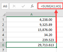
All the decimal points now line up underneath each other.  Cell A5 has three decimal places and this would throw the alignment out normally, but using the ‘?’ character aligns everything perfectly.

Using Literal Characters Within the Format String

You can add any literal character into your format string by preceding it with a backslash ().

Suppose that you want to show a particular currency indicator for your numbers which is not based on your locale.  The problem is that if you use a currency indicator, Excel automatically refers to your local and changes it to the one appropriate for the locale that is set on the Windows Control Panel.  This could have implications if your Excel application is being distributed in other countries and you want to ensure that whatever the locale is, the currency indicator is always the same.

You may also want to indicate that the numbers are in millions in the following example:

Sheets("Sheet1").Range("A1:A6").NumberFormat = "$#,##0.00 m"

This will produce the following results on your worksheet:

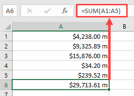
In using a backslash to display literal characters, you do not need to use a backslash for each individual character within a string. You can use:

Sheets("Sheet1").Range("A1:A6").NumberFormat = "$#,##0.00 mill"

This will display ‘mill’ after every number within the formatted range.

You can use most characters as literals, but not reserved characters such as 0, #,?

Use of Commas in a Format String

We have already seen that commas can be used to create thousands separators for large numbers, but they can also be used in another way.

By using them at the end of the numeric part of the format string, they act as scalers of thousands. In other words, they will divide each number by 1,000 every time there is a comma.

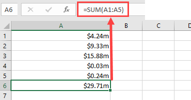
In the example data, we are showing it with an indicator that it is in millions. By inserting one comma into the format string, we can show those numbers divided by 1,000.

Sheets("Sheet1").Range("A1:A6").NumberFormat = "$#,##0.00,m"

This will show the numbers divided by 1,000 although the original number will still be in background in the cell.

If you put two commas in the format string, then the numbers will be divided by a million

Sheets("Sheet1").Range("A1:A6").NumberFormat = "$#,##0.00,,m"

This will be the result using only one comma (divide by 1,000):

VBA Coding Made Easy

Stop searching for VBA code online. Learn more about AutoMacro — A VBA Code Builder that allows beginners to code procedures from scratch with minimal coding knowledge and with many time-saving features for all users!

Learn More

Creating Conditional Formatting within the Format String

You could set up conditional formatting on the front end of Excel, but you can also do it within your VBA code, which means that you can manipulate the format string programmatically to make changes.

You can use up to four sections within your format string.  Each section is delimited by a semicolon (;). The four sections correspond to positive, negative, zero, and text

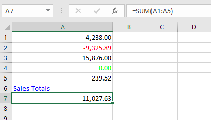
Range("A1:A7").NumberFormat = "#,##0.00;[Red]-#,##0.00;[Green] #,##0.00;[Blue]”

In this example, we use the same hash, comma, and zero characters to provide thousand separators and two decimal points, but we now have different sections for each type of value.

The first section is for positive numbers and is no different to what we have already seen previously in terms of format.

The second section for negative numbers introduces a color (Red) which is held within a pair of square brackets. The format is the same as for positive numbers except that a minus (-) sign has been added in front.

The third section for zero numbers uses a color (Green) within square brackets with the numeric string the same as for positive numbers.

The final section is for text values, and all that this needs is a color (Blue) again within square brackets

This is the result of applying this format string:

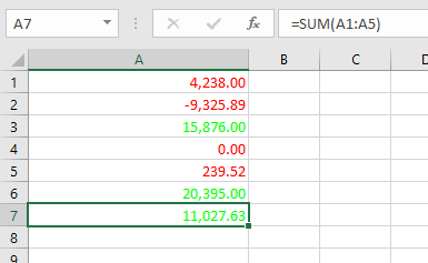
You can go further with conditions within the format string.  Suppose that you wanted to show every positive number above 10,000 as green, and every other number as red you could use this format string:

Range("A1:A7").NumberFormat = "[>=10000][Green]#,##0.00;[<10000][Red]#,##0.00"

This format string includes conditions for >=10000 set in square brackets so that green will only be used where the number is greater than or equal to 10000

This is the result:

Using Fractions in Formatting Strings

Fractions are not often used in spreadsheets, since they normally equate to decimals which everyone is familiar with.

However, sometimes they do serve a purpose. This example will display dollars and cents:

Range("A1:A7").NumberFormat = "#,##0 "" dollars and "" 00/100 ""  cents """

This is the result that will be produced:

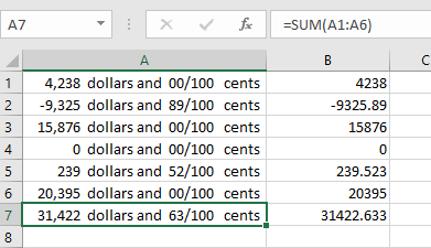
Remember that in spite of the numbers being displayed as text, they are still there in the background as numbers and all the Excel formulas can still be used on them.

Date and Time Formats

Dates are actually numbers and you can use formats on them in the same way as for numbers.  If you format a date as a numeric number, you will see a large number to the left of the decimal point and a number of decimal places. The number to the left of the decimal point shows the number of days starting at 01-Jan-1900, and the decimal places show the time based on 24hrs

MsgBox Format(Now(), "dd-mmm-yyyy")

This will format the current date to show ’08-Jul-2020’. Using ‘mmm’ for the month displays the first three characters of the month name.  If you want the full month name then you use ‘mmmm’

You can include times in your format string:

MsgBox Format(Now(), "dd-mmm-yyyy hh:mm AM/PM")

This will display ’08-Jul-2020 01:25 PM’

‘hh:mm’ represents hours and minutes and AM/PM uses a 12-hour clock as opposed to a 24-hour clock.

You can incorporate text characters into your format string:

MsgBox Format(Now(), "dd-mmm-yyyy hh:mm AM/PM"" today""")

This will display ’08-Jul-2020 01:25 PM today’

You can also use literal characters using a backslash in front in the same way as for numeric format strings.

VBA Programming | Code Generator does work for you!

Predefined Formats

Excel has a number of built-in formats for both numbers and dates that you can use in your code.  These mainly reflect what is available on the number formatting front end, although some of them go beyond what is normally available on the pop-up window.  Also, you do not have the flexibility over number of decimal places, or whether thousands separators are used.

General Number

This format will display the number exactly as it is

MsgBox Format(1234567.89, "General Number")

The result will be 1234567.89

Currency

MsgBox Format(1234567.894, "Currency")

This format will add a currency symbol in front of the number e.g. $, £ depending on your locale, but it will also format the number to 2 decimal places and will separate the thousands with commas.

The result will be $1,234,567.89

Fixed

MsgBox Format(1234567.894, "Fixed")

This format displays at least one digit to the left but only two digits to the right of the decimal point.

The result will be 1234567.89

Standard

MsgBox Format(1234567.894, "Standard")

This displays the number with the thousand separators, but only to two decimal places.

The result will be 1,234,567.89

AutoMacro | Ultimate VBA Add-in | Click for Free Trial!

Percent

MsgBox Format(1234567.894, "Percent")

The number is multiplied by 100 and a percentage symbol (%) is added at the end of the number.  The format displays to 2 decimal places

The result will be 123456789.40%

Scientific

MsgBox Format(1234567.894, "Scientific")

This converts the number to Exponential format

The result will be 1.23E+06

Yes/No

MsgBox Format(1234567.894, "Yes/No")

This displays ‘No’ if the number is zero, otherwise displays ‘Yes’

The result will be ‘Yes’

True/False

MsgBox Format(1234567.894, "True/False")

This displays ‘False’ if the number is zero, otherwise displays ‘True’

The result will be ‘True’

AutoMacro | Ultimate VBA Add-in | Click for Free Trial!

On/Off

MsgBox Format(1234567.894, "On/Off")

This displays ‘Off’ if the number is zero, otherwise displays ‘On’

The result will be ‘On’

General Date

MsgBox Format(Now(), "General Date")

This will display the date as date and time using AM/PM notation.  How the date is displayed depends on your settings in the Windows Control Panel (Clock and Region | Region). It may be displayed as ‘mm/dd/yyyy’ or ‘dd/mm/yyyy’

The result will be ‘7/7/2020 3:48:25 PM’

Long Date

MsgBox Format(Now(), "Long Date")

This will display a long date as defined in the Windows Control Panel (Clock and Region | Region).  Note that it does not include the time.

The result will be ‘Tuesday, July 7, 2020’

Medium Date

MsgBox Format(Now(), "Medium Date")

This displays a date as defined in the short date settings as defined by locale in the Windows Control Panel.

The result will be ’07-Jul-20’

AutoMacro | Ultimate VBA Add-in | Click for Free Trial!

Short Date

MsgBox Format(Now(), "Short Date")

Displays a short date as defined in the Windows Control Panel (Clock and Region | Region). How the date is displayed depends on your locale. It may be displayed as ‘mm/dd/yyyy’ or ‘dd/mm/yyyy’

The result will be ‘7/7/2020’

Long Time

MsgBox Format(Now(), "Long Time")

Displays a long time as defined in Windows Control Panel (Clock and Region | Region).

The result will be ‘4:11:39 PM’

Medium Time

MsgBox Format(Now(), "Medium Time")

Displays a medium time as defined by your locale in the Windows Control Panel. This is usually set as 12-hour format using hours, minutes, and seconds and the AM/PM format.

The result will be ’04:15 PM’

Short Time

MsgBox Format(Now(), "Short Time")

Displays a medium time as defined in Windows Control Panel (Clock and Region | Region). This is usually set as 24-hour format with hours and minutes

The result will be ’16:18’

AutoMacro | Ultimate VBA Add-in | Click for Free Trial!

Dangers of Using Excel’s Pre-Defined Formats in Dates and Times

The use of the pre-defined formats for dates and times in Excel VBA is very dependent on the settings in the Windows Control Panel and also what the locale is set to

Users can easily alter these settings, and this will have an effect on how your dates and times are displayed in Excel

For example, if you develop an Excel application which uses pre-defined formats within your VBA code, these may change completely if a user is in a different country or using a different locale to you.  You may find that column widths do not fit the date definition, or on a user form the Active X control such as a combo box (drop down) control is too narrow for the dates and times to be displayed properly.

You need to consider where the audience is geographically when you develop your Excel application

User-Defined Formats for Numbers

There are a number of different parameters that you can use when defining your format string:

Character	Description
Null String	No formatting
0	Digit placeholder. Displays a digit or a zero. If there is a digit for that position then it displays the digit otherwise it displays 0. If there are fewer digits than zeros, then you will get leading or trailing zeros. If there are more digits after the decimal point than there are zeros, then the number is rounded to the number of decimal places shown by the zeros. If there are more digits before the decimal point than zeros these will be displayed normally.
#	Digit placeholder. This displays a digit or nothing. It works the same as the zero placeholder above, except that leading and trailing zeros are not displayed. For example 0.75 would be displayed using zero placeholders, but this would be .75 using # placeholders.
. Decimal point.	Only one permitted per format string. This character depends on the settings in the Windows Control Panel.
%	Percentage placeholder. Multiplies number by 100 and places % character where it appears in the format string
, (comma)	Thousand separator. This is used if 0 or # placeholders are used and the format string contains a comma. One comma to the left of the decimal point indicates round to the nearest thousand. E.g. ##0, Two adjacent commas to the left of the thousand separator indicate rounding to the nearest million. E.g. ##0,,
E- E+	Scientific format. This displays the number exponentially.
: (colon)	Time separator – used when formatting a time to split hours, minutes and seconds.
/	Date separator – this is used when specifying a format for a date
– + £ $ ( )	Displays a literal character. To display a character other than listed here, precede it with a backslash ()

User-Defined Formats for Dates and Times

These characters can all be used in you format string when formatting dates and times:

Character	Meaning
c	Displays the date as ddddd and the time as ttttt
d	Display the day as a number without leading zero
dd	Display the day as a number with leading zero
ddd	Display the day as an abbreviation (Sun – Sat)
dddd	Display the full name of the day (Sunday – Saturday)
ddddd	Display a date serial number as a complete date according to Short Date in the International settings of the windows Control Panel
dddddd	Displays a date serial number as a complete date according to Long Date in the International settings of the Windows Control Panel.
w	Displays the day of the week as a number (1 = Sunday)
ww	Displays the week of the year as a number (1-53)
m	Displays the month as a number without leading zero
mm	Displays the month as a number with leading zeros
mmm	Displays month as an abbreviation (Jan-Dec)
mmmm	Displays the full name of the month (January – December)
q	Displays the quarter of the year as a number (1-4)
y	Displays the day of the year as a number (1-366)
yy	Displays the year as a two-digit number
yyyy	Displays the year as four-digit number
h	Displays the hour as a number without leading zero
hh	Displays the hour as a number with leading zero
n	Displays the minute as a number without leading zero
nn	Displays the minute as a number with leading zero
s	Displays the second as a number without leading zero
ss	Displays the second as a number with leading zero
ttttt	Display a time serial number as a complete time.
AM/PM	Use a 12-hour clock and display AM or PM to indicate before or after noon.
am/pm	Use a 12-hour clock and use am or pm to indicate before or after noon
A/P	Use a 12-hour clock and use A or P to indicate before or after noon
a/p	Use a 12-hour clock and use a or p to indicate before or after noon

In a recent task, I was doing filter through VBA on a number column. But that number column had numbers in text format. When I run the VBA script, it didn’t work of course, because the filter was a number and the column had numbers as text. In that case, I needed to convert the text into numbers manually and save it. Then the macro worked perfectly. But I wanted to convert these texts into numbers using the VBA script and I was able to do it. I wanted to share this as if anyone wanted to know how to convert text values into a number using VBA, they can have a look at it.

Convert text to number using Range.NumberFormat method

This first and easiest method. I prefer this method over other methods as it directly converts the selected excel range into number format.

So, if you have a fixed range that you want to convert to text then use this VBA snippet.

Sub ConvertTextToNumber()
 Range("A3:A8").NumberFormat = "General"
 Range("A3:A8").Value = Range("A3:A8").Value
End Sub

When you run the above code it converts the text of range A3:A8 into text.

This code can look more elegant if we write it like this.

Sub ConvertTextToNumber()
 
 With Range("A3:A8")
  .NumberFormat = "General"
  .Value = .Value
 End With

End Sub

How does it work?

Well, it is quite simple. We first change the number format of the range to General. Then we put the value of that range into the same range using VBA. This removes the text formatting completely. Simple, isn’t it?

Change the number of formatting of a dynamic range

In the above code, we changed the text to number in the above code of a fixed range but this will not be the case most of the time. To convert text to a number of dynamic ranges, we can evaluate the last used cell or select the range dynamically.

This is how it would look:

Sub ConvertTextToNumber()
With Range("A3:A" & Cells(Rows.Count, 1).End(xlUp).Row)
.NumberFormat = "General"
 .Value = .Value
End With

Here, I know that the range starts from A3. But I don’t know where it may end.
So I dynamically identify last used excel row that has data in it using the VBA snippet Cells(Rows.Count, 1).End(xlUp).Row. It returns the last used row number that we are concatenating with «A3:A».

Note: This VBA snippet will work on the active workbook and active worksheet. If your code switches through multiple sheets, it would be better to set a range object of the intended worksheet. Like this

Sub ConvertTextToNumber()
 Set Rng = ThisWorkbook.Sheets("Sheet1").Range("A3:A" & Cells(Rows.Count, 1).End(xlUp).Row)
 With Rng
  .NumberFormat = "General"
  .Value = .Value
 End With
End Sub

The above code will always change the text to the number of the sheet1 of the workbook that contains this code.

Loop and CSng to change the text to number

Another method is to loop through each cell and change the cell value to a number using CSng function. Here’s the code.

Sub ConvertTextToNumberLoop()
 Set Rng = ThisWorkbook.Sheets("Sheet1").Range("A3:A" & Cells(Rows.Count, 1).End(xlUp).Row)
 
 For Each cel In Rng.Cells
    cel.Value = CSng(cel.Value)
 Next cel

End Sub

In the above VBA snippet, we are using VBA For loop to iterate over each cell in the range and convert the value of each cell into a number using the CSng function of VBA.

So yeah guys, this is how you can change texts to numbers in Excel using VBA. You can use these snippets to ready your worksheet before you do any number operation on them. I hope I was explanatory enough. You can download the working file here.

Change Text to Number Using VBA.

If you have any doubts regarding this text to number conversion or any other excel/VBA related query, ask in the comments section below.

Related Articles:

How to get Text & Number in Reverse through VBA in Microsoft Excel | To reverse number and text we use loops and mid function in VBA. 1234 will be converted to 4321, «you» will be converted to «uoy». Here’s the snippet.

Format data with custom number formats using VBA in Microsoft Excel | To change the number format of specific columns in excel use this VBA snippet. It coverts the number format of specified to specified format in one click.

Popular Articles:

50 Excel Shortcuts to Increase Your Productivity | Get faster at your task. These 50 shortcuts will make you work even faster on Excel.

The VLOOKUP Function in Excel | This is one of the most used and popular functions of excel that is used to lookup value from different ranges and sheets. 

COUNTIF in Excel 2016 | Count values with conditions using this amazing function. You don’t need filter your data to count specific value. Countif function is essential to prepare your dashboard.

How to Use SUMIF Function in Excel | This is another dashboard essential function. This helps you sum up values on specific conditions.