Vba excel фильтр несколько условий - Word и Excel - помощь в работе с программами

I have 8 variables in column A, 1,2,3,4,5 and A, B, C.
My aim is to filter out A, B, C and display only 1-5.

I can do this using the following code:

My_Range.AutoFilter Field:=1, Criteria1:=Array("1", "2", "3","4","5"), _
    Operator:=xlFilterValues

But what the code does is it filters variables 1 to 5 and displays them.

I want to do the opposite, but yielding the same result, by filtering out A, B, C and showing variables 1 to 5

I tried this code:

My_Range.AutoFilter Field:=1, Criteria1:=Array("<>A", "<>B", "<>C"), _
    Operator:=xlFilterValues

But it did not work.

Why cant I use this code ?

It gives this error:

Run time error 1004 autofilter method of range class failed

How can I perform this?

Igor F.

2,6172 gold badges31 silver badges39 bronze badges

asked Feb 18, 2015 at 4:03

I think (from experimenting — MSDN is unhelpful here) that there is no direct way of doing this. Setting Criteria1 to an Array is equivalent to using the tick boxes in the dropdown — as you say it will only filter a list based on items that match one of those in the array.

Interestingly, if you have the literal values "<>A" and "<>B" in the list and filter on these the macro recorder comes up with

Range.AutoFilter Field:=1, Criteria1:="=<>A", Operator:=xlOr, Criteria2:="=<>B"

which works. But if you then have the literal value "<>C" as well and you filter for all three (using tick boxes) while recording a macro, the macro recorder replicates precisely your code which then fails with an error. I guess I’d call that a bug — there are filters you can do using the UI which you can’t do with VBA.

Anyway, back to your problem. It is possible to filter values not equal to some criteria, but only up to two values which doesn’t work for you:

Range("$A$1:$A$9").AutoFilter Field:=1, Criteria1:="<>A", Criteria2:="<>B", Operator:=xlAnd

There are a couple of workarounds possible depending on the exact problem:

Use a «helper column» with a formula in column B and then filter on that — e.g. =ISNUMBER(A2) or =NOT(A2="A", A2="B", A2="C") then filter on TRUE
If you can’t add a column, use autofilter with Criteria1:=">-65535" (or a suitable number lower than any you expect) which will filter out non-numeric values — assuming this is what you want
Write a VBA sub to hide rows (not exactly the same as an autofilter but it may suffice depending on your needs).

For example:

Public Sub hideABCRows(rangeToFilter As Range)
  Dim oCurrentCell As Range
  On Error GoTo errHandler

  Application.ScreenUpdating = False
  For Each oCurrentCell In rangeToFilter.Cells
    If oCurrentCell.Value = "A" Or oCurrentCell.Value = "B" Or oCurrentCell.Value = "C" Then
      oCurrentCell.EntireRow.Hidden = True
    End If
  Next oCurrentCell

  Application.ScreenUpdating = True
  Exit Sub

errHandler:
    Application.ScreenUpdating = True
End Sub

answered Feb 18, 2015 at 9:03

aucupariaaucuparia

2,03118 silver badges27 bronze badges

I don’t have found any solution on Internet, so I have implemented one.

The Autofilter code with criteria is then

iColNumber = 1
Dim aFilterValueArray() As Variant
Call ConstructFilterValueArray(aFilterValueArray, iColNumber, Array("A", "B", "C"))

ActiveSheet.range(sRange).AutoFilter Field:=iColNumber _
    , Criteria1:=aFilterValueArray _
    , Operator:=xlFilterValues

In fact, the ConstructFilterValueArray() method (not function) get all distinct values that it found in a specific column and remove all values present in last argument.

The VBA code of this method is

'************************************************************
'* ConstructFilterValueArray()
'************************************************************

Sub ConstructFilterValueArray(a() As Variant, iCol As Integer, aRemoveArray As Variant)

    Dim aValue As New Collection
    Call GetDistinctColumnValue(aValue, iCol)
    Call RemoveValueList(aValue, aRemoveArray)
    Call CollectionToArray(a, aValue)

End Sub

'************************************************************
'* GetDistinctColumnValue()
'************************************************************

Sub GetDistinctColumnValue(ByRef aValue As Collection, iCol As Integer)

    Dim sValue As String

    iEmptyValueCount = 0
    iLastRow = ActiveSheet.UsedRange.Rows.Count

    Dim oSheet: Set oSheet = Sheets("X")

    Sheets("Data")
        .range(Cells(1, iCol), Cells(iLastRow, iCol)) _
            .AdvancedFilter Action:=xlFilterCopy _
                          , CopyToRange:=oSheet.range("A1") _
                          , Unique:=True

    iRow = 2
    Do While True
        sValue = Trim(oSheet.Cells(iRow, 1))
        If sValue = "" Then
            If iEmptyValueCount > 0 Then
                Exit Do
            End If
            iEmptyValueCount = iEmptyValueCount + 1
        End If

        aValue.Add sValue
        iRow = iRow + 1
    Loop

End Sub

'************************************************************
'* RemoveValueList()
'************************************************************

Sub RemoveValueList(ByRef aValue As Collection, aRemoveArray As Variant)

    For i = LBound(aRemoveArray) To UBound(aRemoveArray)
        sValue = aRemoveArray(i)
        iMax = aValue.Count
        For j = iMax To 0 Step -1
            If aValue(j) = sValue Then
                aValue.Remove (j)
                Exit For
            End If
        Next j
     Next i

End Sub

'************************************************************
'* CollectionToArray()
'************************************************************

Sub CollectionToArray(a() As Variant, c As Collection)

    iSize = c.Count - 1
    ReDim a(iSize)

    For i = 0 To iSize
        a(i) = c.Item(i + 1)
    Next

End Sub

This code can certainly be improved in returning an Array of String but working with Array in VBA is not easy.

CAUTION: this code work only if you define a sheet named X because CopyToRange parameter used in AdvancedFilter() need an Excel Range !

It’s a shame that Microfsoft doesn’t have implemented this solution in adding simply a new enum as xlNotFilterValues ! … or xlRegexMatch !

answered Jan 18, 2018 at 12:44

schlebeschlebe

3,2885 gold badges38 silver badges49 bronze badges

Alternative using VBA’s Filter function

As an innovative alternative to @schlebe ‘s recent answer, I tried to use the Filter function integrated in VBA, which allows to filter out a given search string setting the third argument to False. All «negative» search strings (e.g. A, B, C) are defined in an array. I read the criteria in column A to a datafield array and basicly execute a subsequent filtering (A — C) to filter these items out.

Code

Sub FilterOut()
Dim ws  As Worksheet
Dim rng As Range, i As Integer, n As Long, v As Variant
' 1) define strings to be filtered out in array
  Dim a()                    ' declare as array
  a = Array("A", "B", "C")   ' << filter out values
' 2) define your sheetname and range (e.g. criteria in column A)
  Set ws = ThisWorkbook.Worksheets("FilterOut")
  n = ws.Range("A" & ws.Rows.Count).End(xlUp).row
  Set rng = ws.Range("A2:A" & n)
' 3) hide complete range rows temporarily
  rng.EntireRow.Hidden = True
' 4) set range to a variant 2-dim datafield array
  v = rng
' 5) code array items by appending row numbers
  For i = 1 To UBound(v): v(i, 1) = v(i, 1) & "#" & i + 1: Next i
' 6) transform to 1-dim array and FILTER OUT the first search string, e.g. "A"
  v = Filter(Application.Transpose(Application.Index(v, 0, 1)), a(0), False, False)
' 7) filter out each subsequent search string, i.e. "B" and "C"
  For i = 1 To UBound(a): v = Filter(v, a(i), False, False): Next i
' 8) get coded row numbers via split function and unhide valid rows
  For i = LBound(v) To UBound(v)
      ws.Range("A" & Split(v(i) & "#", "#")(1)).EntireRow.Hidden = False
  Next i
End Sub

answered Jan 18, 2018 at 22:20

T.M.T.M.

9,2293 gold badges32 silver badges57 bronze badges

An option using AutoFilter

Option Explicit

Public Sub FilterOutMultiple()
    Dim ws As Worksheet, filterOut As Variant, toHide As Range

    Set ws = ActiveSheet
    If Application.WorksheetFunction.CountA(ws.Cells) = 0 Then Exit Sub 'Empty sheet

    filterOut = Split("A B C D E F G")

    Application.ScreenUpdating = False
    With ws.UsedRange.Columns("A")
        If ws.FilterMode Then .AutoFilter
       .AutoFilter Field:=1, Criteria1:=filterOut, Operator:=xlFilterValues
        With .SpecialCells(xlCellTypeVisible)
            If .CountLarge > 1 Then Set toHide = .Cells 'Remember unwanted (A, B, and C)
        End With
       .AutoFilter
        If Not toHide Is Nothing Then
            toHide.Rows.Hidden = True                   'Hide unwanted (A, B, and C)
           .Cells(1).Rows.Hidden = False                'Unhide header
        End If
    End With
    Application.ScreenUpdating = True
End Sub

answered Apr 20, 2018 at 0:01

paul bicapaul bica

10.5k4 gold badges22 silver badges41 bronze badges

Here an option using a list written on some range, populating an array that will be fiiltered. The information will be erased then the columns sorted.

Sub Filter_Out_Values()

'Automation to remove some codes from the list
Dim ws, ws1 As Worksheet
Dim myArray() As Variant
Dim x, lastrow As Long
Dim cell As Range

Set ws = Worksheets("List")
Set ws1 = Worksheets(8)
lastrow = ws.Cells(Application.Rows.Count, 1).End(xlUp).Row

'Go through the list of codes to exclude
For Each cell In ws.Range("A2:A" & lastrow)

    If cell.Offset(0, 2).Value = "X" Then 'If the Code is associated with "X"
        ReDim Preserve myArray(x) 'Initiate array
        myArray(x) = CStr(cell.Value) 'Populate the array with the code
        x = x + 1 'Increase array capacity
        ReDim Preserve myArray(x) 'Redim array
    End If

Next cell

lastrow = ws1.Cells(Application.Rows.Count, 1).End(xlUp).Row
ws1.Range("C2:C" & lastrow).AutoFilter field:=3, Criteria1:=myArray, Operator:=xlFilterValues
ws1.Range("A2:Z" & lastrow).SpecialCells(xlCellTypeVisible).ClearContents
ws1.Range("A2:Z" & lastrow).AutoFilter field:=3

'Sort columns
lastrow = ws1.Cells(Application.Rows.Count, 1).End(xlUp).Row
'Sort with 2 criteria
With ws1.Range("A1:Z" & lastrow)
    .Resize(lastrow).Sort _
    key1:=ws1.Columns("B"), order1:=xlAscending, DataOption1:=xlSortNormal, _
    key2:=ws1.Columns("D"), order1:=xlAscending, DataOption1:=xlSortNormal, _
    Header:=xlYes, MatchCase:=False, Orientation:=xlTopToBottom, SortMethod:=xlPinYin
End With

End Sub

answered Feb 13, 2019 at 11:38

This works for me:
This is a criteria over two fields/columns (9 and 10), this filters rows with values >0 on column 9 and rows with values 4, 7, and 8 on column 10. lastrow is the number of rows on the data section.

ActiveSheet.Range("$A$1:$O$" & lastrow).AutoFilter Field:=9, Criteria1:=">0", Operator:=xlAnd
ActiveSheet.Range("$A$1:$O$" & lastrow).AutoFilter Field:=10, Criteria1:=Arr("4","7","8"), Operator:=xlFilterValues

h3t1

1,1142 gold badges18 silver badges29 bronze badges

answered May 6, 2020 at 20:37

Okay, I solved it.

I’ve smashed my head about this problem several times over the years, but I’ve solved it.

All we need to do is look at all the values that are actually IN the filter range, and if they’re not on the list of values we want to filter out, we add them to the «Filter For this item» list.

To note about this code:

I wrote this to act on multiple sheets, and I’m not going to change that as I’m at work and don’t have time. I’m sure you can figure it out.
I don’t think you need to work in Option base 1… But I am, so if you run into issues… might be that.
Despite how many hundreds of thousands of times it’s checking and rechecking the same arrays, it’s remarkably fast.
I’m sure there is a way to redim KeepArray, but I didn’t have time to consider it.

Option Explicit
Option Base 1
Sub FilterTable()
    
    Dim WS As Worksheet
    Dim L As Long
    Dim I As Long
    Dim N As Long
    Dim tbl As ListObject
    Dim tblName As String
    Dim filterArray
    Dim SrcArray
    Dim KeepArray(1 To 5000) ' you might be able to figure out a way to redim this easiely later on.. for now I'm just oversizing it.

    N = 0
    filterArray = Array("FilterMeOut007", _
                        "FilterMeOut006", _
                        "FilterMeOut005", _
                        "FilterMeOut004", _
                        "FilterMeOut003", _
                        "FilterMeOut002", _
                        "FilterMeOut001")


    For Each WS In ThisWorkbook.Worksheets
        Debug.Print WS.Name
        If Left(WS.Name, 4) = "AR -" Then
            With WS
                tblName = Replace(WS.Name, " ", "_")
                Set tbl = WS.ListObjects(tblName)
                SrcArray = tbl.ListColumns(1).DataBodyRange
                For I = 1 To UBound(SrcArray, 1)
                    If Not ExistsInArray(KeepArray, SrcArray(I, 1)) _
                        And Not ExistsInArray(filterArray, SrcArray(I, 1)) Then
                            N = N + 1
                            KeepArray(N) = SrcArray(I, 1)
                    End If
                Next I
                tbl.DataBodyRange.AutoFilter Field:=1, Criteria1:=KeepArray, Operator:=xlFilterValues
            End With
        End If
    Next WS
End Sub
Function ExistsInArray(arr, Val) As Boolean
    Dim I As Long
    ExistsInArray = False
    For I = LBound(arr) To UBound(arr)
        If arr(I) = Val Then
            ExistsInArray = True
            Exit Function
        End If
    Next I
End Function

Please let me know if you run into any errors with this as I’d like to stress test and debug it as much as possible in the future to make it as portable as possible. I picture using it a lot.

answered Feb 16 at 2:31

Please check this one for filtering out values in a range; It works.

Selection.AutoFilter field:=33, Criteria1:="<>Array(IN1R,IN2R,INDA)", Operator:=xlFilterValues

Actually, the above code did not work. Hence I give a loop to hide the entire row whenever the active cell has the value that I am searching for.

For each cell in selection
    If cell.value = “IN1R” or cell.value = “INR2” or cell.value = “INDA” then
    Else
        Activecell.Entirerow.Hidden = True
    End if
Next

answered Apr 24, 2021 at 10:00

Источник

In this Article

Create AutoFilter in VBA
AutoFilter with Field and Criteria Parameters
AutoFilter with Field and Multiple Criteria Values
AutoFilter Data Range with Multiple Criteria
The Operator Parameter Values of AutoFilter method

In VBA, you can use Excel’s AutoFilter to filter a range of cells or an Excel table.

Note: If you want to learn how to use an advanced filter in VBA, click here: VBA Advanced Filter

Create AutoFilter in VBA

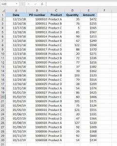
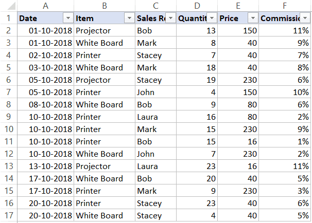
First, we will demonstrate how to AutoFilter a range, so a user can filter the data. The data that we will use in the examples is in Image 1:

Here is the code for creating AutoFilter:

Sheet1.Range("A1:E1").AutoFilter

In order to enable AutoFilter, we need to specify the header of the range, in our case A1:E1, and use the AutoFilter method of the object Range. As a result, our data range has filters activated:

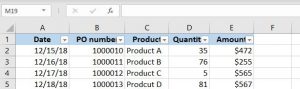
Image 2. AutoFilter enabled for the data

AutoFilter with Field and Criteria Parameters

VBA also allows you to automatically filter a certain field with certain values.

In order to do this, you have to use parameters Field and Criteria1 of the method AutoFilter. In this example, we want to filter the third column (Product) for Product A only. Here is the code:

Sheet1.Range("A1:E1").AutoFilter Field:=3, _
                                 Criteria1:="Product A"

In the Field parameter, you can set the number of the column in the range (not in Excel), while in Criteria1 you can put the value which you want to filter. After executing the code, our table looks like this:

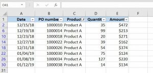
Image 3. AutoFilter with field and criteria

As you can see, only rows with Product A in the third column are displayed in the data range.

AutoFilter with Field and Multiple Criteria Values

If you want to filter one field with several values, you need to use the parameter Operator of the AutoFilter method. To filter multiple values, you need to set Operator to xlFilterValues and also to put all the values of Criteria in an Array. In this example, we filter the Product column for Product A and Product B. Here is the code example:

Sheet1.Range("A1:E1").AutoFilter Field:=3, _
                                 Criteria1:=Array("Product A", "Product B"), _
                                 Operator:=xlFilterValues

When we execute the code, we get only rows with Product A and Product B, as you can see in Image 4:

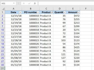
Image 4. AutoFilter with multiple criteria values

AutoFilter Data Range with Multiple Criteria

If you want to filter a field with multiple criteria, you have to use Criteria1 and Criteria2 parameters, but also the Operator xlAnd.

In the next example, we will filter the first column (Date) for dates in December 2018. Therefore, we have two criteria: a date greater than 12/01/18 and less than 12/31/18. This is the code:

Sheet1.Range("A1:E1").AutoFilter Field:=1, _
                                 Criteria1:=">=12/01/2018", _
                                 Operator:=xlAnd, _
                                 Criteria2:="<=12/31/2018"

When we execute the code, you can see that only dates in December are displayed in the data range:

Image 5. AutoFilter with multiple criteria for the field

The Operator Parameter Values of AutoFilter method

In the next table. you can see all possible values of the Operator parameter of AutoFilter method and their descriptions:

Operator	Description
xlAnd	Includes multiple criteria – Criteria1 and Criteria 2
xlOr	Includes one of the multiple criteria – Criteria1 or Criteria 2
xlTop10Items	Filters a certain number of highest ranked values (number specified in Criteria1)
xlBottom10Items	Filters a certain number of lowest ranked values (number specified in Criteria1)
xlTop10Percent	Filters a certain percentage of highest ranked values (% specified in Criteria1)
xlBottom10Percent	Filters a certain percentage of lowest ranked values (% specified in Criteria1)
xlFilterValues	Includes multiple criteria values with Array
xlFilterCellColor	Filters cells for colors
xlFilterFontColor	Filters cells for font colors
xlFIlterIcon	Filters icons
xlFilterDynamic	Filter dynamic values

VBA Coding Made Easy

Stop searching for VBA code online. Learn more about AutoMacro — A VBA Code Builder that allows beginners to code procedures from scratch with minimal coding knowledge and with many time-saving features for all users!

Learn More!

Источник

На чтение 11 мин. Просмотров 34.3k.

Итог: научиться создавать макросы, использовать фильтры на диапазоны и таблицы с помощью метода AutoFilter VBA. Статья содержит ссылки на примеры для фильтрации различных типов данных, включая текст, цифры, даты, цвета и значки.

Уровень мастерства: средний

Содержание

Скачать файл
Написание макросов для фильтров
Макро-рекордер — твой друг (или враг)
Метод автофильтрации
Написание кода автофильтра
Автофильтр не является дополнением
Как установить номер поля динамически
Используйте таблицы Excel с фильтрами
Фильтры и типы данных
Почему метод автофильтрации такой сложный?

Скачать файл

Файл Excel, содержащий код, можно скачать ниже. Этот файл содержит код для фильтрации различных типов данных и типов фильтров.

VBA AutoFilters Guide.xlsm (100.5 KB)

Написание макросов для фильтров

Фильтры являются отличным инструментом для анализа данных в
Excel. Для большинства аналитиков и частых пользователей Excel фильтры являются
частью нашей повседневной жизни. Мы используем раскрывающиеся меню фильтров для
применения фильтров к отдельным столбцам в наборе данных. Это помогает нам
связывать цифры с отчетами и проводить исследование наших данных.

Фильтрация также может быть трудоемким процессом. Особенно,
когда мы применяем фильтры к нескольким столбцам на больших листах или фильтруем
данные, чтобы затем копировать / вставлять их в другие листы или книги.

В этой статье объясняется, как создавать макросы для
автоматизации процесса фильтрации. Это обширное руководство по методу
автофильтра в VBA.

У меня также есть статьи с примерами для различных фильтров и типов данных, в том числе: пробелы, текст, числа, даты, цвета и значки, и очищающие фильтры.

Макро-рекордер — твой друг (или враг)

Мы можем легко получить код VBA для фильтров, включив
макро-рекордер, а затем применив один или несколько фильтров к диапазону /
таблице.

Вот шаги для создания макроса фильтра с помощью устройства
записи макросов:

Включите рекордер макросов:
1. Вкладка «Разработчик»> «Запись макроса».
2. Дайте макросу имя, выберите, где вы хотите сохранить код, и нажмите ОК.
Примените один или несколько фильтров, используя раскрывающиеся меню фильтров.
Остановите рекордер.
Откройте редактор VB (вкладка «Разработчик»> Visual Basic) для просмотра кода.

Если вы уже использовали макрос-рекордер для этого процесса,
то вы знаете, насколько он может быть полезен. Тем более, что наши критерии
фильтрации становятся более сложными.

Код будет выглядеть примерно так:

Sub Filters_Macro_Recorder()
'
' Filters_Macro_Recorder Macro
'

'
    ActiveSheet.ListObjects("tblData").Range.AutoFilter Field:=4, Criteria1:= _
        "Product 2"
    ActiveSheet.ListObjects("tblData").Range.AutoFilter Field:=4
    ActiveSheet.ListObjects("tblData").Range.AutoFilter Field:=5, Criteria1:= _
        ">=500", Operator:=xlAnd, Criteria2:="<=1000"
End Sub

Мы видим, что каждая строка использует метод AutoFilter для
применения фильтра к столбцу. Он также содержит информацию о критериях фильтра.

Метод автофильтрации

Метод AutoFilter используется для очистки и применения
фильтров к одному столбцу в диапазоне или таблице в VBA. Он автоматизирует
процесс применения фильтров через выпадающие меню фильтров и делает, чтобы все работало.

Его можно использовать для применения фильтров к нескольким
столбцам путем написания нескольких строк кода, по одной для каждого столбца.
Мы также можем использовать Автофильтр, чтобы применить несколько критериев
фильтрации к одному столбцу, так же, как в выпадающем меню фильтра, установив
несколько флажков или указав диапазон дат.

Написание кода автофильтра

Вот пошаговые инструкции по написанию строки кода для автофильтра.

Шаг 1: Ссылка на диапазон или таблицу

Метод AutoFilter является частью объекта Range. Поэтому мы
должны ссылаться на диапазон или таблицу, к которым применяются фильтры на
листе. Это будет весь диапазон, к которому применяются фильтры.

Следующие примеры включают / отключают фильтры в диапазоне B3: G1000 на листе автофильтра.

Sub AutoFilter_Range()
'Автофильтр является членом объекта Range
  
  'Ссылка на весь диапазон, к которому применяются фильтры
  'Автофильтр включает / выключает фильтры, когда параметры не указаны.
  Sheet1.Range("B3:G1000").AutoFilter
  
  'Полностью квалифицированный справочник, начиная с уровня Workbook
  ThisWorkbook.Worksheets("AutoFilter Guide").Range("B3:G1000").AutoFilter

End Sub

Вот пример использования таблиц Excel.

Sub AutoFilter_Table()
'Автофильтры на таблицах работают одинаково.

Dim lo As ListObject 'Excel Table

  'Установить переменную ListObject (Table)
  Set lo = Sheet1.ListObjects(1)
  
  'Автофильтр является членом объекта Range
  'Родителем объекта Range является объект List
  lo.Range.AutoFilter
  
End Sub

Метод AutoFilter имеет 5 необязательных параметров, которые
мы рассмотрим далее. Если мы не укажем ни один из параметров, как в приведенных
выше примерах, метод AutoFilter включит / выключит фильтры для указанного
диапазона. Это переключение. Если фильтры включены, они будут выключены, и
наоборот.

Диапазоны или таблицы?

Фильтры работают одинаково как для обычных диапазонов, так и для таблиц
Excel.

Я отдаю предпочтение методу использования таблиц, потому что
нам не нужно беспокоиться об изменении ссылок на диапазон при увеличении или
уменьшении таблицы. Однако код будет одинаковым для обоих объектов. В остальных
примерах кода используются таблицы Excel, но вы можете легко изменить это для
обычных диапазонов.

5 (или 6) параметров автофильтра

Метод
AutoFilter имеет 5 (или 6) необязательных параметров, которые используются для
указания критериев фильтрации для столбца. Вот список параметров.

Страница справки MSDN

Мы можем использовать комбинацию этих параметров, чтобы
применять различные критерии фильтрации для разных типов данных. Первые четыре
являются наиболее важными, поэтому давайте посмотрим, как их применять.

Шаг 2: Параметр поля

Первый параметр — это Field. Для параметра Field мы указываем число, которое является номером столбца, к которому будет применяться фильтр. Это номер столбца в диапазоне фильтра, который является родителем метода AutoFilter. Это НЕ номер столбца на рабочем листе.

В приведенном ниже примере поле 4 является столбцом
«Продукт», поскольку это 4-й столбец в диапазоне фильтра / таблице.

Фильтр столбца очищается, когда мы указываем только параметр
Field, а другие критерии отсутствуют.

Мы также можем использовать переменную для параметра Field и
установить ее динамически. Я объясню это более подробно ниже.

Шаг 3: Параметры критериев

Существует два параметра, которые можно использовать для указания фильтра Критерии, Criteria1 и Criteria2 . Мы используем комбинацию этих параметров и параметра Operator для разных типов фильтров. Здесь все становится сложнее, поэтому давайте начнем с простого примера.

'Фильтровать столбец «Продукт» для одного элемента
lo.Range.AutoFilter Field:=4, Criteria1:="Product 2"

Это то же самое, что выбрать один элемент из списка флажков в раскрывающемся меню фильтра.

Общие правила для Criteria1 и Criteria2

Значения, которые мы указываем для Criteria1 и Criteria2,
могут быть хитрыми. Вот несколько общих рекомендаций о том, как ссылаться на
значения параметра Criteria.

Значением критерия является строка, заключенная в кавычки. Есть несколько исключений, когда критерии являются постоянными для периода времени даты и выше / ниже среднего.
При указании фильтров для отдельных чисел или дат форматирование чисел должно соответствовать форматированию чисел, применяемому в диапазоне / таблице.
Оператор сравнения больше / меньше чем также включен в кавычки перед числом.
Кавычки также используются для фильтров для пробелов «=» и не пробелов «<>».

'Фильтр на дату, большую или равную 1 января 2015 г.
lo.Range.AutoFilter Field:=1, Criteria1:=">=1/1/2015"

' Оператор сравнения> = находится внутри кавычек
' для параметра Criteria1.

' Форматирование даты в коде соответствует форматированию
' применяется к ячейкам на листе.

Шаг 4: Параметр оператора

Что если мы хотим выбрать несколько элементов из
раскрывающегося списка фильтров? Или сделать фильтр для диапазона дат или
чисел?

Для этого нам нужен Operator . Параметр Operator используется для указания типа фильтра, который мы хотим применить. Он может варьироваться в зависимости от типа данных в столбце. Для
Operator должна использоваться одна из следующих 11 констант.

Вот ссылка на страницу справки MSDN, которая содержит список констант для перечисления XlAutoFilterOperator.

Operator используется в сочетании с Criteria1 и / или Criteria2, в зависимости от типа данных и типа фильтра. Вот несколько примеров.

'Фильтр для списка нескольких элементов, оператор - xlFilterValues
lo.Range.AutoFilter _
          Field:=iCol, _
          Criteria1:=Array("Product 4", "Product 5", "Product 6"), _
          Operator:=xlFilterValues

'Фильтр для диапазона дат (между датами), оператор xlAnd
lo.Range.AutoFilter _
          Field:=iCol, _
          Criteria1:=">=1/1/2014", _
          Operator:=xlAnd, _
          Criteria2:="<=12/31/2015"

Это основы написания строки кода для метода AutoFilter. Будет сложнее с различными типами данных.

Итак, я привел много примеров ниже, которые содержат большинство комбинаций критериев и операторов для разных типов фильтров.

Автофильтр не является дополнением

При запуске строки кода автофильтра сначала удаляются все
фильтры, примененные к этому столбцу (полю), а затем применяются критерии
фильтра, указанные в строке кода.

Это означает, что это не дополнение. Следующие 2 строки НЕ создадут фильтр для Продукта 1 и Продукта 2. После запуска макроса столбец Продукт будет отфильтрован только для Продукта 2.

'Автофильтр НЕ ДОБАВЛЯЕТ. Это сначала любые фильтры, применяемые
'в столбце перед применением нового фильтра
lo.Range.AutoFilter Field:=4, Criteria1:="Product 3"
  
'Эта строка кода отфильтрует столбец только для продукта 2
'Фильтр для Продукта 3 выше будет очищен при запуске этой линии.
lo.Range.AutoFilter Field:=4, Criteria1:="Product 2"

Если вы хотите применить фильтр с несколькими критериями к одному столбцу, вы можете указать это с помощью параметров
Criteria и Operator .

Как установить номер поля динамически

Если мы добавим / удалим / переместим столбцы в диапазоне
фильтра, то номер поля для отфильтрованного столбца может измениться. Поэтому я
стараюсь по возможности избегать жесткого кодирования числа для параметра
Field.

Вместо этого мы можем использовать переменную и использовать некоторый код, чтобы найти номер столбца по его имени. Вот два примера для обычных диапазонов и таблиц.

Sub Dynamic_Field_Number()
'Методы, чтобы найти и установить поле на основе имени столбца.
  
Dim lo As ListObject
Dim iCol As Long
  
  'Установить ссылку на первую таблицу на листе
  Set lo = Sheet1.ListObjects(1)
  
  'Установить поле фильтра
  iCol = lo.ListColumns("Product").Index
  
  'Использовать функцию соответствия для регулярных диапазонов
  'iCol = WorksheetFunction.Match("Product", Sheet1.Range("B3:G3"), 0)

  'Использовать переменную для значения параметра поля
  lo.Range.AutoFilter Field:=iCol, Criteria1:="Product 3"

End Sub

Номер столбца будет найден при каждом запуске макроса. Нам
не нужно беспокоиться об изменении номера поля при перемещении столбца. Это
экономит время и предотвращает ошибки (беспроигрышный вариант)!

Используйте таблицы Excel с фильтрами

Использование таблиц Excel дает множество преимуществ,
особенно при использовании метода автофильтрации. Вот несколько основных
причин, по которым я предпочитаю таблицы.

Нам не нужно переопределять диапазон в VBA, поскольку диапазон данных изменяет размер (строки / столбцы добавляются / удаляются). На всю таблицу ссылается объект ListObject.
Данные в таблице легко ссылаться после применения фильтров. Мы можем использовать свойство DataBodyRange для ссылки на видимые строки для копирования / вставки, форматирования, изменения значений и т.д.
Мы можем иметь несколько таблиц на одном листе и, следовательно, несколько диапазонов фильтров. С обычными диапазонами у нас может быть только один отфильтрованный диапазон на лист.
Код для очистки всех фильтров в таблице легче написать.

Фильтры и типы данных

Параметры раскрывающегося меню фильтра изменяются в
зависимости от типа данных в столбце. У нас есть разные фильтры для текста,
чисел, дат и цветов. Это создает МНОГО различных комбинаций операторов и
критериев для каждого типа фильтра.

Я создал отдельные посты для каждого из этих типов фильтров.
Посты содержат пояснения и примеры кода VBA.

Как очистить фильтры с помощью VBA
Как отфильтровать пустые и непустые клетки
Как фильтровать текст с помощью VBA
Как фильтровать числа с помощью VBA
Как отфильтровать даты с помощью VBA
Как отфильтровать цвета и значки с помощью VBA

Файл в разделе загрузок выше содержит все эти примеры кода в одном месте. Вы можете добавить его в свою личную книгу макросов и использовать макросы в своих проектах.

Почему метод автофильтрации такой сложный?

Этот пост был вдохновлен вопросом от Криса, участника The
VBA Pro Course. Комбинации Критерии и Операторы могут быть запутанными и
сложными. Почему это?

Ну, фильтры развивались на протяжении многих лет. Мы увидели много новых типов фильтров, представленных в Excel 2010, и эта функция продолжает улучшаться. Однако параметры метода автофильтра не изменились. Они отлично подходят для совместимости со старыми версиями, но также означает, что новые типы фильтров работают с существующими параметрами.

Большая часть кода фильтра имеет смысл, но сначала может быть
сложно разобраться. К счастью, у нас есть макро рекордер, чтобы помочь с этим.

Я надеюсь, что вы можете использовать эту статью и файл Excel в качестве руководства по написанию макросов для фильтров. Автоматизация фильтров может сэкономить нам и нашим пользователям массу времени, особенно при использовании этих методов в более крупном проекте автоматизации данных.

Источник

Zaharius

0 / 0 / 0

Регистрация: 16.11.2011

Сообщений: 40

04.11.2012, 15:32. Показов 16358. Ответов 5

Метки нет (Все метки)

В одном из листов книги Excel содержатся данные, третий столбец которых содержит значения дат.
Необходимо через VBA задать фильтрацию данных таким образом, чтобы были выбраны все строки, в которых дата в третьем столбце имеет значение между определёнными датами (скажем между 05.01.2012 и 25.01.2012) , либо не содержит никакого значения.
Напрашивается что-то вроде: Код:

Visual Basic

1	ActiveSheet.Cells.AutoFilter Field:=3, Criteria1:=">=01/05/2012", Operator:=xlAnd, Criteria2:="<=05/25/2012", Operator:=xlOr, Criteria3:="="

Но на третий критерий VBA выдаёт ошибку. Что можно тут сделать?

Programming Эксперт 94731 / 64177 / 26122 Регистрация: 12.04.2006 Сообщений: 116,782	04.11.2012, 15:32
5

5468 / 1148 / 50

Регистрация: 15.09.2012

Сообщений: 3,514

04.11.2012, 15:44

Zaharius, иногда можно найти ответ на вопрос, просто посмотрев встроенную справку по VBA.

Чтобы посмотреть справку по VBA:

перейдите в VBA;
2 варианта:
- в поле в правом вверхнем углу вставьте этот текст: AutoFilter и нажмите клавишу Enter, появится список статей, связанных с AutoFilter. Найдите какую-нибудь статью, где можно посмотреть синтаксис команды AutoFilter;
- в коде поставьте курсор на слово AutoFilter и нажмите клавишу F1. Появится справка по команде AutoFilter. Посмотрите синтаксис этой команды.

У команды AutoFilter только два критерия для фильтрации.
Поэтому вам нужно использовать другие средства для достижения вашей задачи.

Смысл фильтрации заключается в скрытии строк, которые не содержат нужной информации.
Поэтому вам нужно определить, какие строки надо скрыть.

0 / 0 / 0

Регистрация: 16.11.2011

Сообщений: 40

04.11.2012, 16:35

[ТС]

УРА!!! Ваша информация просто бесценна!!! Правда, обычно в таких случаях ещё рекомендуют погуглить .
Только я, собственно, интересуюсь, может кто подскажет мне «другие средства для достижения задачи».
P.S. Если Вы, Скрипт, кините ссылку на Help или MSDN, где эта задача решается, — с меня пиво

призрак

3261 / 889 / 119

Регистрация: 11.05.2012

Сообщений: 1,702

Записей в блоге: 2

04.11.2012, 16:54

расширенный фильтр
опять же, в справке

Скрипт

5468 / 1148 / 50

Регистрация: 15.09.2012

Сообщений: 3,514

04.11.2012, 17:03

Код работает в активном листе в столбце C.

Visual Basic

Sub Procedure_1()
 
    'Здесь указываем, с какой строки начинаются даты.
    Const lStart As Long = 2
 
    Dim dateCellData As Date
    Dim lLastRow As Long
    Dim i As Long
    
    'Определяем последнюю строку с данными на активном листе.
    'What:="?" - символ "?" означает любой один символ.
    'SearchDirection:=xlPrevious - xlPrevious - означает, что поиск будет идти
    'с конца в начало.
    lLastRow = Cells.Find(What:="?", After:=Range("A1"), LookIn:=xlValues, _
        LookAt:=xlPart, SearchOrder:=xlByRows, SearchDirection:=xlPrevious, _
        MatchCase:=False, SearchFormat:=False).Row
        
    'Отключаем обновление монитора, чтобы код работал быстрее.
    Application.ScreenUpdating = False
        
    'Двигаемся по 3 столбцу со строки, в которой начинаются даты, до
    'последней строки с данными на листе
    For i = lStart To lLastRow Step 1
    
        'Проверяем, дата в ячейке или нет.
        If IsDate(Cells(i, "C").Value) = True Then
        
            'Чтобы каждый раз не обращаться к ячейке (т.к. это больше времени занимает),
            'поместим данные из ячейки в переменную dateCellData.
            dateCellData = Cells(i, "C").Value
            
            'Смотрим, в каком диапазоне находится дата в ячейке.
            If dateCellData >= "01/05/2012" And _
                    dateCellData <= "05/25/2012" Then
                
                'Скрываем строку
                Rows(i).Hidden = True
        
            End If
        
        'Если не дата в ячейке, то скрываем строку.
        Else
            Rows(i).Hidden = True
        End If
        
    Next i
 
    'Включаем обновление монитора.
    Application.ScreenUpdating = True
    
    'Сообщение, что работа кода завершена.
    MsgBox "Фильтрация произведена!", vbInformation
 
End Sub

ikki, для расширенного фильтра нужно добавлять строки, названия столбцов. Мне кажется, что это неудобства может доставить.

1121 / 229 / 36

Регистрация: 15.03.2010

Сообщений: 698

04.11.2012, 19:16

Сообщение от Zaharius

Необходимо через VBA задать фильтрацию данных таким образом, чтобы были выбраны все строки, в которых дата в третьем столбце имеет значение между определёнными датами (скажем между 05.01.2012 и 25.01.2012) , либо не содержит никакого значения.

Выдели в строках ячейки для расчета условий и отфильтруй по ним.

Источник

A lot of Excel functionalities are also available to be used in VBA – and the Autofilter method is one such functionality.

If you have a dataset and you want to filter it using a criterion, you can easily do it using the Filter option in the Data ribbon.

And if you want a more advanced version of it, there is an advanced filter in Excel as well.

Then Why Even Use the AutoFilter in VBA?

If you just need to filter data and do some basic stuff, I would recommend stick to the inbuilt Filter functionality that Excel interface offers.

You should use VBA Autofilter when you want to filter the data as a part of your automation (or if it helps you save time by making it faster to filter the data).

For example, suppose you want to quickly filter the data based on a drop-down selection, and then copy this filtered data into a new worksheet.

While this can be done using the inbuilt filter functionality along with some copy-paste, it can take you a lot of time to do this manually.

In such a scenario, using VBA Autofilter can speed things up and save time.

Note: I will cover this example (on filtering data based on a drop-down selection and copying into a new sheet) later in this tutorial.

Excel VBA Autofilter Syntax
- Example: Filtering Data based on a Text condition
- Example: Multiple Criteria (AND/OR) in the Same Column
- Example: Multiple Criteria With Different Columns
- Example: Filter Top 10 Records Using the AutoFilter Method
- Example: Filter Top 10 Percent Using the AutoFilter Method
- Example: Using Wildcard Characters in Autofilter
- Example: Copy Filtered Rows into a New Sheet
- Example: Filter Data based on a Cell Value
Turn Excel AutoFilter ON/OFF using VBA
Check if AutoFilter is Already Applied
Show All Data
Using AutoFilter on Protected Sheets

Excel VBA Autofilter Syntax

Expression. AutoFilter( _Field_ , _Criteria1_ , _Operator_ , _Criteria2_ , _VisibleDropDown_ )

Expression: This is the range on which you want to apply the auto filter.
Field: [Optional argument] This is the column number that you want to filter. This is counted from the left in the dataset. So if you want to filter data based on the second column, this value would be 2.
Criteria1: [Optional argument] This is the criteria based on which you want to filter the dataset.
Operator: [Optional argument] In case you’re using criteria 2 as well, you can combine these two criteria based on the Operator. The following operators are available for use: xlAnd, xlOr, xlBottom10Items, xlTop10Items, xlBottom10Percent, xlTop10Percent, xlFilterCellColor, xlFilterDynamic, xlFilterFontColor, xlFilterIcon, xlFilterValues
Criteria2: [Optional argument] This is the second criteria on which you can filter the dataset.
VisibleDropDown: [Optional argument] You can specify whether you want the filter drop-down icon to appear in the filtered columns or not. This argument can be TRUE or FALSE.

Apart from Expression, all the other arguments are optional.

In case you don’t use any argument, it would simply apply or remove the filter icons to the columns.

Sub FilterRows()
Worksheets("Filter Data").Range("A1").AutoFilter
End Sub

The above code would simply apply the Autofilter method to the columns (or if it’s already applied, it will remove it).

This simply means that if you can not see the filter icons in the column headers, you will start seeing it when this above code is executed, and if you can see it, then it will be removed.

In case you have any filtered data, it will remove the filters and show you the full dataset.

Now let’s see some examples of using Excel VBA Autofilter that will make it’s usage clear.

Example: Filtering Data based on a Text condition

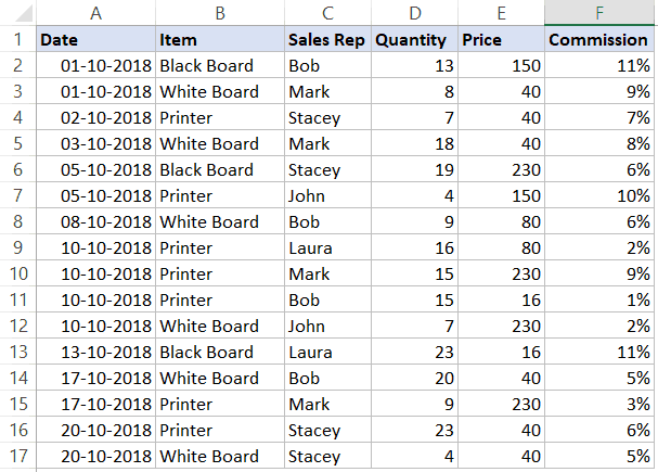
Suppose you have a dataset as shown below and you want to filter it based on the ‘Item’ column.

The below code would filter all the rows where the item is ‘Printer’.

Sub FilterRows()
Worksheets("Sheet1").Range("A1").AutoFilter Field:=2, Criteria1:="Printer"
End Sub

The above code refers to Sheet1 and within it, it refers to A1 (which is a cell in the dataset).

Note that here we have used Field:=2, as the item column is the second column in our dataset from the left.

Now if you’re thinking – why do I need to do this using a VBA code. This can easily be done using inbuilt filter functionality.

You’re right!

If this is all you want to do, better used the inbuilt Filter functionality.

But as you read the remaining tutorial, you’ll see that this can be combined with some extra code to create powerful automation.

But before I show you those, let me first cover a few examples to show you what all the AutoFilter method can do.

Click here to download the example file and follow along.

Example: Multiple Criteria (AND/OR) in the Same Column

Suppose I have the same dataset, and this time I want to filter all the records where the item is either ‘Printer’ or ‘Projector’.

The below code would do this:

Sub FilterRowsOR()
Worksheets("Sheet1").Range("A1").AutoFilter Field:=2, Criteria1:="Printer", Operator:=xlOr, Criteria2:="Projector"
End Sub

Note that here I have used the xlOR operator.

This tells VBA to use both the criteria and filter the data if any of the two criteria are met.

Similarly, you can also use the AND criteria.

For example, if you want to filter all the records where the quantity is more than 10 but less than 20, you can use the below code:

Sub FilterRowsAND()
Worksheets("Sheet1").Range("A1").AutoFilter Field:=4, Criteria1:=">10", _
    Operator:=xlAnd, Criteria2:="<20"
End Sub

Example: Multiple Criteria With Different Columns

Suppose you have the following dataset.

With Autofilter, you can filter multiple columns at the same time.

For example, if you want to filter all the records where the item is ‘Printer’ and the Sales Rep is ‘Mark’, you can use the below code:

Sub FilterRows()
With Worksheets("Sheet1").Range("A1")
.AutoFilter field:=2, Criteria1:="Printer"
.AutoFilter field:=3, Criteria1:="Mark"
End With
End Sub

Example: Filter Top 10 Records Using the AutoFilter Method

Suppose you have the below dataset.

Below is the code that will give you the top 10 records (based on the quantity column):

Sub FilterRowsTop10()
ActiveSheet.Range("A1").AutoFilter Field:=4, Criteria1:="10", Operator:=xlTop10Items
End Sub

In the above code, I have used ActiveSheet. You can use the sheet name if you want.

Note that in this example, if you want to get the top 5 items, just change the number in Criteria1:=”10″ from 10 to 5.

So for top 5 items, the code would be:

Sub FilterRowsTop5()
ActiveSheet.Range("A1").AutoFilter Field:=4, Criteria1:="5", Operator:=xlTop10Items
End Sub

It may look weird, but no matter how many top items you want, the Operator value always remains xlTop10Items.

Similarly, the below code would give you the bottom 10 items:

Sub FilterRowsBottom10()
ActiveSheet.Range("A1").AutoFilter Field:=4, Criteria1:="10", Operator:=xlBottom10Items
End Sub

And if you want the bottom 5 items, change the number in Criteria1:=”10″ from 10 to 5.

Example: Filter Top 10 Percent Using the AutoFilter Method

Suppose you have the same data set (as used in the previous examples).

Below is the code that will give you the top 10 percent records (based on the quantity column):

Sub FilterRowsTop10()
ActiveSheet.Range("A1").AutoFilter Field:=4, Criteria1:="10", Operator:=xlTop10Percent
End Sub

In our dataset, since we have 20 records, it will return the top 2 records (which is 10% of the total records).

Example: Using Wildcard Characters in Autofilter

Suppose you have a dataset as shown below:

If you want to filter all the rows where the item name contains the word ‘Board’, you can use the below code:

Sub FilterRowsWildcard()
Worksheets("Sheet1").Range("A1").AutoFilter Field:=2, Criteria1:="*Board*"
End Sub

In the above code, I have used the wildcard character * (asterisk) before and after the word ‘Board’ (which is the criteria).

An asterisk can represent any number of characters. So this would filter any item that has the word ‘board’ in it.

Example: Copy Filtered Rows into a New Sheet

If you want to not only filter the records based on criteria but also copy the filtered rows, you can use the below macro.

It copies the filtered rows, adds a new worksheet, and then pastes these copied rows into the new sheet.

Sub CopyFilteredRows()
Dim rng As Range
Dim ws As Worksheet
If Worksheets("Sheet1").AutoFilterMode = False Then
MsgBox "There are no filtered rows"
Exit Sub
End If
Set rng = Worksheets("Sheet1").AutoFilter.Range
Set ws = Worksheets.Add
rng.Copy Range("A1")
End Sub

The above code would check if there are any filtered rows in Sheet1 or not.

If there are no filtered rows, it will show a message box stating that.

And if there are filtered rows, it will copy those, insert a new worksheet, and paste these rows on that newly inserted worksheet.

Example: Filter Data based on a Cell Value

Using Autofilter in VBA along with a drop-down list, you can create a functionality where as soon as you select an item from the drop-down, all the records for that item are filtered.

Something as shown below:

Click here to download the example file and follow along.

This type of construct can be useful when you want to quickly filter data and then use it further in your work.

Below is the code that will do this:

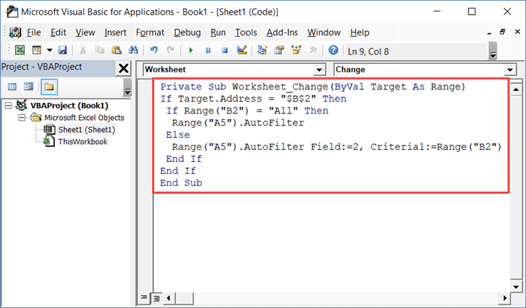
Private Sub Worksheet_Change(ByVal Target As Range)
If Target.Address = "$B$2" Then
 If Range("B2") = "All" Then
  Range("A5").AutoFilter
 Else
  Range("A5").AutoFilter Field:=2, Criteria1:=Range("B2")
 End If
End If
End Sub

This is a worksheet event code, which gets executed only when there is a change in the worksheet and the target cell is B2 (where we have the drop-down).

Also, an If Then Else condition is used to check if the user has selected ‘All’ from the drop down. If All is selected, the entire data set is shown.

This code is NOT placed in a module.

Instead, it needs to be placed in the backend of the worksheet that has this data.

Here are the steps to put this code in the worksheet code window:

Open the VB Editor (keyboard shortcut – ALT + F11).
In the Project Explorer pane, double-click on the Worksheet name in which you want this filtering functionality.
In the worksheet code window, copy and paste the above code.
Close the VB Editor.

Now when you use the drop-down list, it will automatically filter the data.

This is a worksheet event code, which gets executed only when there is a change in the worksheet and the target cell is B2 (where we have the drop-down).

Also, an If Then Else condition is used to check if the user has selected ‘All’ from the drop down. If All is selected, the entire data set is shown.

Turn Excel AutoFilter ON/OFF using VBA

When applying Autofilter to a range of cells, there may already be some filters in place.

You can use the below code turn off any pre-applied auto filters:

Sub TurnOFFAutoFilter()
  Worksheets("Sheet1").AutoFilterMode = False
End Sub

This code checks the entire sheets and removes any filters that have been applied.

If you don’t want to turn off filters from the entire sheet but only from a specific dataset, use the below code:

Sub TurnOFFAutoFilter()
  If Worksheets("Sheet1").Range("A1").AutoFilter Then
    Worksheets("Sheet1").Range("A1").AutoFilter
  End If
End Sub

The above code checks whether there are already filters in place or not.

If filters are already applied, it removes it, else it does nothing.

Similarly, if you want to turn on AutoFilter, use the below code:

Sub TurnOnAutoFilter()
  If Not Worksheets("Sheet1").Range("A4").AutoFilter Then
    Worksheets("Sheet1").Range("A4").AutoFilter
  End If
End Sub

Check if AutoFilter is Already Applied

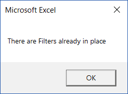
If you have a sheet with multiple datasets and you want to make sure you know that there are no filters already in place, you can use the below code.

Sub CheckforFilters()
If ActiveSheet.AutoFilterMode = True Then
MsgBox "There are Filters already in place"
Else
MsgBox "There are no filters"
End If
End Sub

This code uses a message box function that displays a message ‘There are Filters already in place’ when it finds filters on the sheet, else it shows ‘There are no filters’.

Show All Data

If you have filters applied to the dataset and you want to show all the data, use the below code:

Sub ShowAllData()
If ActiveSheet.FilterMode Then ActiveSheet.ShowAllData
End Sub

The above code checks whether the FilterMode is TRUE or FALSE.

If it’s true, it means a filter has been applied and it uses the ShowAllData method to show all the data.

Note that this does not remove the filters. The filter icons are still available to be used.

Using AutoFilter on Protected Sheets

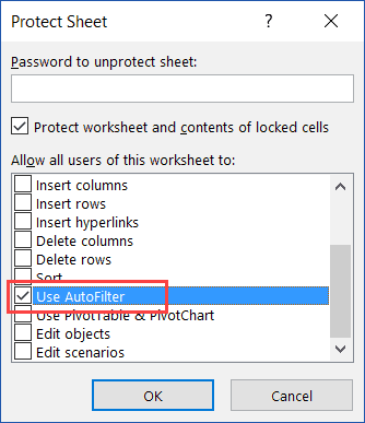
By default, when you protect a sheet, the filters won’t work.

In case you already have filters in place, you can enable AutoFilter to make sure it works even on protected sheets.

To do this, check the Use Autofilter option while protecting the sheet.

While this works when you already have filters in place, in case you try to add Autofilters using a VBA code, it won’t work.

Since the sheet is protected, it wouldn’t allow any macro to run and make changes to the Autofilter.

So you need to use a code to protect the worksheet and make sure auto filters are enabled in it.

This can be useful when you have created a dynamic filter (something I covered in the example – ‘Filter Data based on a Cell Value’).

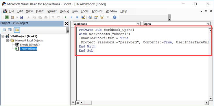
Below is the code that will protect the sheet, but at the same time, allow you to use Filters as well as VBA macros in it.

Private Sub Workbook_Open()
With Worksheets("Sheet1")
.EnableAutoFilter = True
.Protect Password:="password", Contents:=True, UserInterfaceOnly:=True
End With
End Sub

This code needs to be placed in ThisWorkbook code window.

Here are the steps to put the code in ThisWorkbook code window:

Open the VB Editor (keyboard shortcut – ALT + F11).
In the Project Explorer pane, double-click on the ThisWorkbook object.
In the code window that opens, copy and paste the above code.

As soon as you open the workbook and enable macros, it will run the macro automatically and protect Sheet1.

However, before doing that, it will specify ‘EnableAutoFilter = True’, which means that the filters would work in the protected sheet as well.

Also, it sets the ‘UserInterfaceOnly’ argument to ‘True’. This means that while the worksheet is protected, the VBA macros code would continue to work.

You May Also Like the Following VBA Tutorials:

Excel VBA Loops.
Filter Cells with Bold Font Formatting.
Recording a Macro.
Sort Data Using VBA.
Sort Worksheet Tabs in Excel.

Источник