
Вставка формулы со ссылками в стиле A1 и R1C1 в ячейку (диапазон) из кода VBA Excel. Свойства Range.FormulaLocal и Range.FormulaR1C1Local.
Свойство Range.FormulaLocal
FormulaLocal — это свойство объекта Range, которое возвращает или задает формулу на языке пользователя, используя ссылки в стиле A1.
В качестве примера будем использовать диапазон A1:E10, заполненный числами, которые необходимо сложить построчно и результат отобразить в столбце F:

Примеры вставки формул суммирования в ячейку F1:
|
Range(«F1»).FormulaLocal = «=СУММ(A1:E1)» Range(«F1»).FormulaLocal = «=СУММ(A1;B1;C1;D1;E1)» |
Пример вставки формул суммирования со ссылками в стиле A1 в диапазон F1:F10:
|
Sub Primer1() Dim i As Byte For i = 1 To 10 Range(«F» & i).FormulaLocal = «=СУММ(A» & i & «:E» & i & «)» Next End Sub |
В этой статье я не рассматриваю свойство Range.Formula, но если вы решите его применить для вставки формулы в ячейку, используйте англоязычные функции, а в качестве разделителей аргументов — запятые (,) вместо точек с запятой (;):
|
Range(«F1»).Formula = «=SUM(A1,B1,C1,D1,E1)» |
После вставки формула автоматически преобразуется в локальную (на языке пользователя).
Свойство Range.FormulaR1C1Local
FormulaR1C1Local — это свойство объекта Range, которое возвращает или задает формулу на языке пользователя, используя ссылки в стиле R1C1.
Формулы со ссылками в стиле R1C1 можно вставлять в ячейки рабочей книги Excel, в которой по умолчанию установлены ссылки в стиле A1. Вставленные ссылки в стиле R1C1 будут автоматически преобразованы в ссылки в стиле A1.
Примеры вставки формул суммирования со ссылками в стиле R1C1 в ячейку F1 (для той же таблицы):
|
‘Абсолютные ссылки в стиле R1C1: Range(«F1»).FormulaR1C1Local = «=СУММ(R1C1:R1C5)» Range(«F1»).FormulaR1C1Local = «=СУММ(R1C1;R1C2;R1C3;R1C4;R1C5)» ‘Ссылки в стиле R1C1, абсолютные по столбцам и относительные по строкам: Range(«F1»).FormulaR1C1Local = «=СУММ(RC1:RC5)» Range(«F1»).FormulaR1C1Local = «=СУММ(RC1;RC2;RC3;RC4;RC5)» ‘Относительные ссылки в стиле R1C1: Range(«F1»).FormulaR1C1Local = «=СУММ(RC[-5]:RC[-1])» Range(«F2»).FormulaR1C1Local = «=СУММ(RC[-5];RC[-4];RC[-3];RC[-2];RC[-1])» |
Пример вставки формул суммирования со ссылками в стиле R1C1 в диапазон F1:F10:
|
‘Ссылки в стиле R1C1, абсолютные по столбцам и относительные по строкам: Range(«F1:F10»).FormulaR1C1Local = «=СУММ(RC1:RC5)» ‘Относительные ссылки в стиле R1C1: Range(«F1:F10»).FormulaR1C1Local = «=СУММ(RC[-5]:RC[-1])» |
Так как формулы с относительными ссылками и относительными по строкам ссылками в стиле R1C1 для всех ячеек столбца F одинаковы, их можно вставить сразу, без использования цикла, во весь диапазон.
In this Article
- Formulas in VBA
- Macro Recorder and Cell Formulas
- VBA FormulaR1C1 Property
- Absolute References
- Relative References
- Mixed References
- VBA Formula Property
- VBA Formula Tips
- Formula With Variable
- Formula Quotations
- Assign Cell Formula to String Variable
- Different Ways to Add Formulas to a Cell
- Refresh Formulas
This tutorial will teach you how to create cell formulas using VBA.
Formulas in VBA
Using VBA, you can write formulas directly to Ranges or Cells in Excel. It looks like this:
Sub Formula_Example()

    'Assign a hard-coded formula to a single cell
    Range("b3").Formula = "=b1+b2"

    'Assign a flexible formula to a range of cells
    Range("d1:d100").FormulaR1C1 = "=RC2+RC3"

End Sub
There are two Range properties you will need to know:
- .Formula – Creates an exact formula (hard-coded cell references). Good for adding a formula to a single cell.
- .FormulaR1C1 – Creates a flexible formula. Good for adding formulas to a range of cells where cell references should change.
For simple formulas, it’s fine to use the .Formula Property. However, for everything else, we recommend using the Macro Recorder…
Macro Recorder and Cell Formulas
The Macro Recorder is our go-to tool for writing cell formulas with VBA. You can simply:
- Start recording
- Type the formula (with relative / absolute references as needed) into the cell & press enter
- Stop recording
- Open VBA and review the formula, adapting as needed and copying+pasting the code where needed.
I find it’s much easier to enter a formula into a cell than to type the corresponding formula in VBA.
Notice a couple of things:
- The Macro Recorder will always use the .FormulaR1C1 property
- The Macro Recorder recognizes Absolute vs. Relative Cell References
VBA FormulaR1C1 Property
The FormulaR1C1 property uses R1C1-style cell referencing (as opposed to the standard A1-style you are accustomed to seeing in Excel).
Here are some examples:
Sub FormulaR1C1_Examples()

    'Reference D5 (Absolute)
    '=$D$5
    Range("a1").FormulaR1C1 = "=R5C4"

    'Reference D5 (Relative) from cell A1
    '=D5
    Range("a1").FormulaR1C1 = "=R[4]C[3]"

    'Reference D5 (Absolute Row, Relative Column) from cell A1
    '=D$5
    Range("a1").FormulaR1C1 = "=R5C[3]"

    'Reference D5 (Relative Row, Absolute Column) from cell A1
    '=$D5
    Range("a1").FormulaR1C1 = "=R[4]C4"

End Sub
Notice that the R1C1-style cell referencing allows you to set absolute or relative references.
Absolute References
In standard A1 notation an absolute reference looks like this: “=$C$2”. In R1C1 notation it looks like this: “=R2C3”.
To create an Absolute cell reference using R1C1-style type:
- R + Row number
- C + Column number
Example: R2C3 would represent cell $C$2 (C is the 3rd column).
    'Reference D5 (Absolute)
    '=$D$5
    Range("a1").FormulaR1C1 = "=R5C4"
Relative References
Relative cell references are cell references that “move” when the formula is moved.
In standard A1 notation they look like this: “=C2”. In R1C1 notation, you use brackets [] to offset the cell reference from the current cell.
Example: Entering formula “=R[1]C[1]” in cell B3 would reference cell D4 (the cell 1 row below and 1 column to the right of the formula cell).
Use negative numbers to reference cells above or to the left of the current cell.
    'Reference D5 (Relative) from cell A1
    '=D5
    Range("a1").FormulaR1C1 = "=R[4]C[3]"
Mixed References
Cell references can be partially relative and partially absolute. Example:
    'Reference D5 (Relative Row, Absolute Column) from cell A1
    '=$D5
    Range("a1").FormulaR1C1 = "=R[4]C4"
VBA Coding Made Easy
Stop searching for VBA code online. Learn more about AutoMacro — A VBA Code Builder that allows beginners to code procedures from scratch with minimal coding knowledge and with many time-saving features for all users!

Learn More
VBA Formula Property
When setting formulas with the .Formula Property you will always use A1-style notation. You enter the formula just like you would in an Excel cell, except surrounded by quotations:
    'Assign a hard-coded formula to a single cell
    Range("b3").Formula = "=b1+b2"
VBA Formula Tips
Formula With Variable
When working with Formulas in VBA, it’s very common to want to use variables within the cell formulas. To use variables, you use & to combine the variables with the rest of the formula string. Example:
Sub Formula_Variable()
    Dim colNum As Long
    colNum = 4

    Range("a1").FormulaR1C1 = "=R1C" & colNum & "+R2C" & colNum

End Sub
VBA Programming | Code Generator does work for you!
Formula Quotations
If you need to add a quotation (“) within a formula, enter the quotation twice (“”):
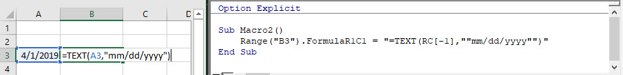
Sub Macro2()
    Range("B3").FormulaR1C1 = "=TEXT(RC[-1],""mm/dd/yyyy"")"
End Sub
A single quotation (“) signifies to VBA the end of a string of text. Whereas a double quotation (“”) is treated like a quotation within the string of text.
Similarly, use 3 quotation marks (“””) to surround a string with a quotation mark (“)
MsgBox """Use 3 to surround a string with quotes"""
' This will print <"Use 3 to surround a string with quotes"> immediate window
Assign Cell Formula to String Variable
We can read the formula in a given cell or range and assign it to a string variable:
'Assign Cell Formula to Variable
Dim strFormula as String
strFormula = Range("B1").Formula
Different Ways to Add Formulas to a Cell
Here are a few more examples for how to assign a formula to a cell:
- Directly Assign Formula
- Define a String Variable Containing the Formula
- Use Variables to Create Formula
Sub MoreFormulaExamples ()
' Alternate ways to add SUM formula
' to cell B1
'
  Dim strFormula as String
  Dim cell as Range
  dim fromRow as long, toRow as long

  Set cell = Range("B1")

  ' Directly assigning a String
  cell.Formula = "=SUM(A1:A10)"

  ' Storing string to a variable
  ' and assigning to "Formula" property
  strFormula = "=SUM(A1:A10)"
  cell.Formula = strFormula

  ' Using variables to build a string
  ' and assigning it to "Formula" property
  fromRow = 1
  toRow   = 10
  strFormula = "=SUM(A" & fromValue & ":A" & toValue & ")
  cell.Formula = strFormula
End Sub
Refresh Formulas
As a reminder, to refresh formulas, you can use the Calculate command:
CalculateTo refresh single formula, range, or entire worksheet use .Calculate instead:
Sheets("Sheet1").Range("a1:a10").CalculateIn this lesson you can learn how to add a formula to a cell using vba. There are several ways to insert formulas to cells automatically. We can use properties like Formula, Value and FormulaR1C1 of the Range object. This post explains five different ways to add formulas to cells.
Table of contents
How to add formula to cell using VBA
Add formula to cell and fill down using VBA
Add sum formula to cell using VBA
How to add If formula to cell using VBA
Add formula to cell with quotes using VBA
Add Vlookup formula to cell using VBA
We use formulas to calculate various things in Excel. Sometimes you may need to enter the same formula to hundreds or thousands of rows or columns only changing the row numbers or columns. For an example let’s consider this sample Excel sheet.
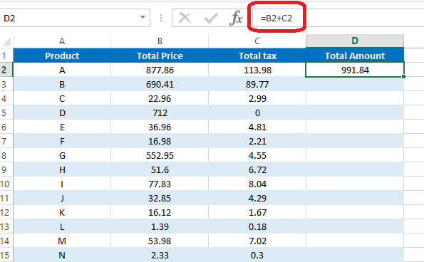
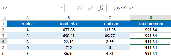
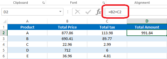
In this Excel sheet I have added a very simple formula to the D2 cell.
=B2+C2
So what if we want to add similar formulas for all the rows in column D. So the D3 cell will have the formula as =B3+C3 and D4 will have the formula as =B4+D4 and so on. Luckily we don’t need to type the formulas manually in all rows. There is a much easier way to do this. First select the cell containing the formula. Then take the cursor to the bottom right corner of the cell. Mouse pointer will change to a + sign. Then left click and drag the mouse until the end of the rows.
However if you want to add the same formula again and again for lots of Excel sheets then you can use a VBA macro to speed up the process. First let’s look at how to add a formula to one cell using vba.
How to add formula to cell using VBA
Lets see how we can enter above simple formula(=B2+C2) to cell D2 using VBA
In this method we are going to use the Formula property of the Range object.
Sub AddFormula_Method1()
Dim WS As Worksheet
Set WS = Worksheets(«Sheet1»)
WS.Range(«D2»).Formula = «=B2+C2»
End Sub
We can also use the Value property of the Range object to add a formula to a cell.
Sub AddFormula_Method2()
Dim WS As Worksheet
Set WS = Worksheets(«Sheet1»)
WS.Range(«D2»).Value = «=B2+C2»
End Sub
Next method is to use the FormulaR1C1 property of the Range object. There are few different ways to use FormulaR1C1 property. We can use absolute reference, relative reference or use both types of references inside the same formula.
In the absolute reference method cells are referred to using numbers. Excel sheets have numbers for each row. So you should think similarly for columns. So column A is number 1. Column B is number 2 etc. Then when writing the formula use R before the row number and C before the column number. So the cell A1 is referred to by R1C1. A2 is referred to by R2C1. B3 is referred to by R3C2 etc.
This is how you can use the absolute reference.
Sub AddFormula_Method3A()
Dim WS As Worksheet
Set WS = Worksheets(«Sheet1»)
WS.Range(«D2»).FormulaR1C1 = «=R2C2+R2C3»
End Sub
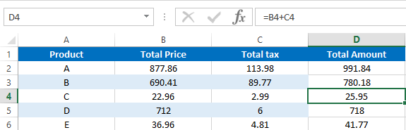
If you use the absolute reference, the formula will be added like this.
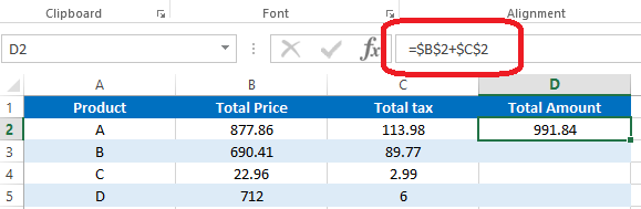
If you use the manual drag method explained above to fill down other rows, then the same formula will be copied to all the rows.
In Majority cases this is not how you want to fill down the formula. However this won’t happen in the relative method. In the relative method, cells are given numbers relative to the cell where the formula is entered. You should use negative numbers when referring to the cells in upward direction or left. Also the numbers should be placed within the square brackets. And you can omit [0] when referring to cells on the same row or column. So you can use RC[-2] instead of R[0]C[-2]. The macro recorder also generates relative reference type code, if you enter a formula to a cell while enabling the macro recorder.
Below example shows how to put formula =B2+C2 in D2 cell using relative reference method.
Sub AddFormula_Method3B()
Dim WS As Worksheet
Set WS = Worksheets(«Sheet1»)
WS.Range(«D2»).FormulaR1C1 = «=RC[-2]+RC[-1]»
End Sub
Now use the drag method to fill down all the rows.
You can see that the formulas are changed according to the row numbers.
Also you can use both relative and absolute references in the same formula. Here is a typical example where you need a formula with both reference types.
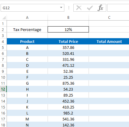
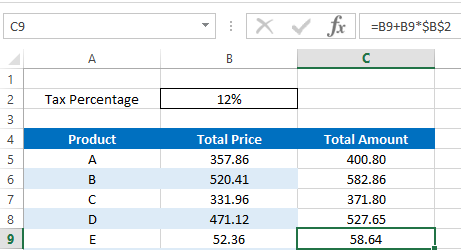
We can add the formula to calculate Total Amount like this.
Sub AddFormula_Method3C()
Dim WS As Worksheet
Set WS = Worksheets(«Sheet2»)
WS.Range(«C5»).FormulaR1C1 = «=RC[-1]+RC[-1]*R2C2»
End Sub
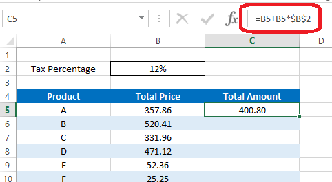
In this formula we have a absolute reference after the * symbol. So when we fill down the formula using the drag method that part will remain the same for all the rows. Hence we will get correct results for all the rows.
Add formula to cell and fill down using VBA
So now you’ve learnt various methods to add a formula to a cell. Next let’s look at how to fill down the other rows with the added formula using VBA.
Assume we have to calculate cell D2 value using =B2+C2 formula and fill down up to 1000 rows. First let’s see how we can modify the first method to do this. Let’s name this subroutine as “AddFormula_Method1_1000Rows”
Sub AddFormula_Method1_1000Rows()
End Sub
Then we need an additional variable for the For Next statement
Dim WS As Worksheet
Dim i As Integer
Next, assign the worksheet to WS variable
Set WS = Worksheets(«Sheet1»)
Now we can add the For Next statement like this.
For i = 2 To 1000
WS.Range(«D» & i).Formula = «=B» & i & «+C» & i
Next i
Here I have used «D» & i instead of D2 and «=B» & i & «+C» & i instead of «=B2+C2». So the formula keeps changing like =B3+C3, =B4+C4, =B5+C5 etc. when iterated through the For Next loop.
Below is the full code of the subroutine.
Sub AddFormula_Method1_1000Rows()
Dim WS As Worksheet
Dim i As Integer
Set WS = Worksheets(«Sheet1»)
For i = 2 To 1000
WS.Range(«D» & i).Formula = «=B» & i & «+C» & i
Next i
End Sub
So that’s how you can use VBA to add formulas to cells with variables.
Next example shows how to modify the absolute reference type of FormulaR1C1 method to add formulas upto 1000 rows.
Sub AddFormula_Method3A_1000Rows()
Dim WS As Worksheet
Dim i As Integer
Set WS = Worksheets(«Sheet1»)
For i = 2 To 1000
WS.Range(«D» & i).FormulaR1C1 = «=R» & i & «C2+R» & i & «C3»
Next i
End Sub
You don’t need to do any change to the formula section when modifying the relative reference type of the FormulaR1C1 method.
Sub AddFormula_Method3B_1000Rows()
Dim WS As Worksheet
Dim i As Integer
Set WS = Worksheets(«Sheet1»)
For i = 2 To 1000
WS.Range(«D» & i).FormulaR1C1 = «=RC[-2]+RC[-1]»
Next i
End Sub
Use similar techniques to modify other two types of subroutines to add formulas for multiple rows. Now you know how to add formulas to cells with a variable. Next let’s look at how to add formulas with some inbuilt functions using VBA.
How to add sum formula to a cell using VBA
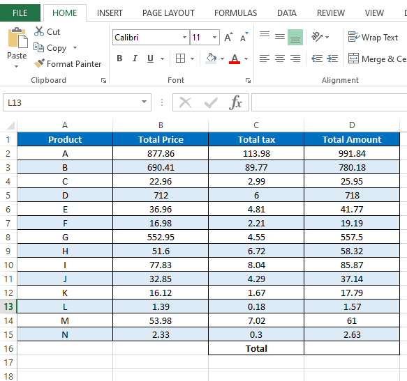
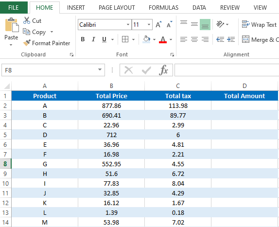
Suppose we want the total of column D in the D16 cell. So this is the formula we need to create.
=SUM(D2:D15)
Now let’s see how to add this using VBA. Let’s name this subroutine as SumFormula.
First let’s declare a few variables.
Dim WS As Worksheet
Dim StartingRow As Long
Dim EndingRow As Long
Assign the worksheet to the variable.
Set WS = Worksheets(«Sheet3»)
Assign the starting row and the ending row to relevant variables.
StartingRow = 2
EndingRow = 1
Then the final step is to create the formula with the above variables.
WS.Range(«D16»).Formula = «=SUM(D» & StartingRow & «:D» & EndingRow & «)»
Below is the full code to add the Sum formula using VBA.
Sub SumFormula()
Dim WS As Worksheet
Dim StartingRow As Long
Dim EndingRow As Long
Set WS = Worksheets(«Sheet3»)
StartingRow = 2
EndingRow = 15
WS.Range(«D16»).Formula = «=SUM(D» & StartingRow & «:D» & EndingRow & «)»
End Sub
How to add If Formula to a cell using VBA
If function is a very popular inbuilt worksheet function available in Microsoft Excel. This function has 3 arguments. Two of them are optional.
Now let’s see how to add a If formula to a cell using VBA. Here is a typical example where we need a simple If function.
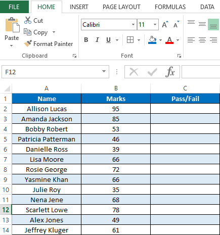
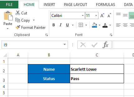
This is the results of students on an examination. Here we have names of students in column A and their marks in column B. Students should get “Pass” if he/she has marks equal or higher than 40. If marks are less than 40 then Excel should show the “Fail” in column C. We can simply obtain this result by adding an If function to column C. Below is the function we need in the C2 cell.
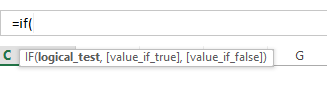
=IF(B2>=40,»Pass»,»Fail»)
Now let’s look at how to add this If Formula to a C2 cell using VBA. Once you know how to add it then you can use the For Next statement to fill the rest of the rows like we did above. We discussed a few different ways to add formulas to a range object using VBA. For this particular example I’m going to use the Formula property of the Range object.
So now let’s see how we can develop this macro. Let’s name this subroutine as “AddIfFormula”
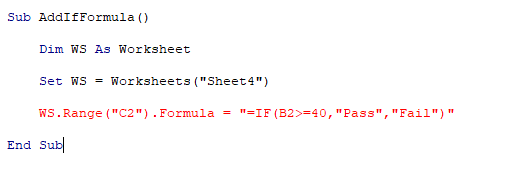
Sub AddIfFormula()
End Sub
However we can’t simply add this If formula using the Formula property like we did before. Because this If formula has quotes inside it. So if we try to add the formula to the cell with quotes, then we get a syntax error.
Add formula to cell with quotes
There are two ways to add the formula to a cell with quotes.
Sub AddIfFormula_Method1()
Dim WS As Worksheet
Set WS = Worksheets(«Sheet4»)
WS.Range(«C2»).Formula = «=IF(B2>=40,»»Pass»»,»»Fail»»)»
End Sub
Sub AddIfFormula_Method2()
Dim WS As Worksheet
Set WS = Worksheets(«Sheet4»)
WS.Range(«C2»).Formula = «=IF(B2>=40,» & Chr(34) & «Pass» & Chr(34) & «,» & Chr(34) & «Fail» & Chr(34) & «)»
End Sub
Add vlookup formula to cell using VBA
Finally I will show you how to add a vlookup formula to a cell using VBA. So I created a very simple example where we can use a Vlookup function. Assume we have this section in the Sheet5 of the same workbook.
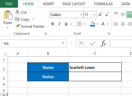
So here when we change the name of the student in the C2 cell, his/her pass or fail status should automatically be shown in the C3 cell. If the original data(data we used in the above “If formula” example) is listed in the Sheet4 then we can write a Vlookup formula for the C3 cell like this.
=VLOOKUP(Sheet5!C2,Sheet4!A2:C200,3,FALSE)
We can use the Formula property of the Range object to add this Vlookup formula to the C3 using VBA.
Sub AddVlookupFormula()
Dim WS As Worksheet
Set WS = Worksheets(«Sheet5»)
WS.Range(«C3»).Formula = «=VLOOKUP(Sheet5!C2,Sheet4!A2:C200,3,FALSE)»
End Sub
Try:
.Formula = "='" & strProjectName & "'!" & Cells(2, 7).Address
If your worksheet name (strProjectName) has spaces, you need to include the single quotes in the formula string.
If this does not resolve it, please provide more information about the specific error or failure.
Update
In comments you indicate you’re replacing spaces with underscores. Perhaps you are doing something like:
strProjectName = Replace(strProjectName," ", "_")
But if you’re not also pushing that change to the Worksheet.Name property, you can expect these to happen:
- The file browse dialog appears
- The formula returns
#REFerror
The reason for both is that you are passing a reference to a worksheet that doesn’t exist, which is why you get the #REF error. The file dialog is an attempt to let you correct that reference, by pointing to a file wherein that sheet name does exist. When you cancel out, the #REF error is expected.
So you need to do:
Worksheets(strProjectName).Name = Replace(strProjectName," ", "_")
strProjectName = Replace(strProjectName," ", "_")
Then, your formula should work.
- Set Formulas for a Cell in VBA
- Address of a Cell in VBA
- Select Cell Range in VBA
- Write in Cells in VBA
- Read From Cells in VBA
- Intersect Cells in VBA
- Replace Values of Non-Contiguous Cells in VBA
- Offset From a Cell in VBA
- Refer to a Cell Address in VBA
- Include All Cells in VBA
- Change Properties of a Cell in VBA
- Find the Last Cell in VBA
- Find the Last Cell Used in a Column in VBA
- Find the Last Cell Used in a Row in VBA
- Copy-Paste Cell Values in VBA
We will introduce different cell functions that can be performed in VBA to achieve different tasks with examples.
Set Formulas for a Cell in VBA
Worksheets of excel contain cells for data storage purposes. These cells are arranged to form rows and columns in the worksheet.
While we involve cell(s) from an excel worksheet for VBA coding, we use a range that includes one or more cells. Some of the essential features related to VBA cells are the following:
- Address of the cell
- Cell range
- Writing in cells
- Reading from cells
- Intersecting cells
- Non-Contiguous cells
- Offsetting from cells
- Referring to a cell address
- Including all cells
- Changing the properties of cells
- Finding the last cell
- Finding the last row number used in a column
- Finding the last column number used in a row
- Copy-pasting a cell
Address of a Cell in VBA
We can identify the address of a cell through A1 notation, in which we include the name of the column letter and write the row number of the cell. In VBA, the range object can be included.
Let us refer to cell B4, as shown below.
# vba
MsgBox Range("B4")
Output:
As shown below, if we want to refer to a cell from another worksheet, we can easily call it by calling the sheet and getting the cell.
# vba
MsgBox Worksheets("Sheet2").Range("B4")
Output:
We can even open another workbook and choose the worksheet from that workbook to get the value of the desired cell, as shown below.
# vba
MsgBox Workbooks("My WorkBook").Worksheets("Sheet2").Range("B2")
Another way to write a cell address is to use the letter R and the row number. Next, write the letter C and the cell’s column number.
This method is called R1C1 notation. Let’s use this notation in our example, as shown below.
#vba
Sub callIt()

Cells(4, 2) = "Added"

End Sub
Output:
Select Cell Range in VBA
We can also select a range of cells by giving range values to the function Range below.
# vba
Range("A1:B13")
We can use the above function to change the style of cells present in that range. Let us go through an example in which we will change the border color of the cells from that range, as shown below.
# vba
Sub callIt()

Range("A1:B13").Borders.Color = RGB(255, 0, 255)

End Sub
Output:
As you can see from the above example, we can easily change the styles using the range function by providing the values of cells.
Write in Cells in VBA
There are many scenarios where we may want to edit or add value to a particular cell. Using VBA, replacing the cell value or adding the cell value is very easy; we can use the range() function.
Then, let us use the range() function to add a value and change it.
# vba
Sub callIt()

Range("B4") = "Value Added"

End Sub
Once the value is added, we will change the value. And we will try to replace the same cell as shown below.
# vba
Sub callIt()

Range("B4") = "Value Changed"

End Sub
Output:
We can also use the Cells method to perform the same function.
# vba
Sub callIt()

Cells(4, 2) = "Value"

End Sub
Output:
If we want to store a range of values, using an array is better than using a simple variable.
Read From Cells in VBA
If we want to read values from a cell, we can use 2 functions. One is the Range, and the other is the Cells. By calling the cell’s address, we can get its value.
We can use the MsgBox method to display our value. Let us go through an example and fetch the value of B4 using the Cells method first.
# vba
Sub callIt()

cellValue = Cells(4, 2)

MsgBox (cellValue)

End Sub
Output:
Let us try to achieve the same thing using the range() method below.
# vba
Sub callIt()

cellValue = Range("B4")

MsgBox (cellValue)

End Sub
Output:
As you can see from the above example, it is very easy to read the values of cells using these two functions.
Intersect Cells in VBA
While working in VBA to create formulas for excel sheets, we may need to find the intersection of 2 ranges and perform specific tasks there. Or we want to place a particular value at the intersection of these 2 ranges.
Space is used between cell addresses and the VBA for the intersecting process.
As shown below, we will go through an example in which we will add a value in the range cells, common between both ranges.
# vba
Sub callIt()

Range("A1:B10 B1:C10") = "Common Cells"

End Sub
Output:
As you can see from the above example, we can easily add or replace the values between the cells that intersect between two ranges.
Replace Values of Non-Contiguous Cells in VBA
There may be some situations where we have to replace the values of the non-contiguous cells. We can easily do that using the range for multiple cells or a single cell.
For non-contiguous cells, put a comma (,) between different cell addresses. Let us go through an example in which we will replace the values of specific cells, as shown below.
# vba
Sub callIt()

Range("A2,C3,B5") = 10

End Sub
Output:
Now, let us change the value of a single non-contiguous cell, as shown below.
# vba
Sub callIt()

Cells(5, 2) = "Hello"

End Sub
Output:
Offset From a Cell in VBA
There may be a situation while working on VBA with excel sheets where we may have a reference cell from which we want to get some offset cell value or replace the value of the cell based on the one cell address.
We can use the offset method to achieve this scenario smoothly.
Let us go through an example in which we will use this function to move 1 column and 1 row using the range method as shown below.
# vba
Sub callIt()

Range("A1").Offset(1, 1) = "A1"

End Sub
Output:
Now, try the same scenario using the Cells method below.
# vba
Sub callIt()

Cells(1, 1).Offset(0, 0) = "A1"

End Sub
Output:
Now, let us imagine if we want to add the values to multiple cells based on the offset value of the range, we can do this as shown below.
# vba
Sub callIt()

Range("A1:B13").Offset(4, 2) = "Completed"

End Sub
Output:
Refer to a Cell Address in VBA
Now, if we want to get the address of a cell, we can quickly get it using the function Address. Let’s go through an example in which we will try to get the address of a specific cell, as shown below.
# vba
Sub callIt()

Set cell = Cells(2, 4)

MsgBox cell.Address

End Sub
Output:
As you can see from the above example, we can easily get the address of any cell using the method address in VBA.
Include All Cells in VBA
There may be situations where we want to clear all the data from all cells. For this scenario, we can write the following code as shown below.
# vba
Sub callIt()

Cells.Clear

End Sub
Output:
As you can see from the above example that we can easily
Change Properties of a Cell in VBA
There may be situations when we have to change the properties of specific cells. VBA provides easy ways to change the properties of any cell.
Let us go through an example in which we will change the font color, as shown below.
# vba
Sub callIt()

Set NewCell = Range("A1")

NewCell.Activate

NewCell.Font.Color = RGB(255, 0, 0)

End Sub
Output:
Now, let us try to change the font family and font size of the cell, as shown below.
# vba
Sub callIt()

Set cell = Range("A1")

cell.Activate

cell.Font.Size = 20
cell.Font.FontStyle = "Courier"

End Sub
Output:
Find the Last Cell in VBA
There may be some situations where we may have to find the last cell of the column or row. We can use Row.count and Column.count in VBA to find the last row of an excel worksheet.
As shown below, let’s go through an example and find the last cell from rows and columns.
# vba
Sub callIt()

MsgBox ("Last cell row wise in the sheet: " & Rows.Count)

MsgBox ("Last cell column wise in the sheet: " & Columns.Count)

End Sub
Output:
As you can see from the above example that it is pretty easy to find the last cell of the row or column by using the simple function count.
Find the Last Cell Used in a Column in VBA
There may be situations when we want to know the last cell used by a column to get an idea of the number of data we are storing.
As shown below, let’s go through an example and find the last cell occupied in specific columns.
# vba
Sub callIt()

MsgBox (Cells(Rows.Count, "B").End(xlUp).Row)

End Sub
Output:
As you can see from the above example, we can find the last cell used with 100% accuracy. VBA is the best method to find these things accurately and not lose any data.
Find the Last Cell Used in a Row in VBA
There may be situations when we want to know the last cell used by a row to get an idea of the number of data we are storing.
As shown below, let us go through an example and find the last cell occupied in a specific row.
# vba
Sub callIt()

MsgBox (Cells(9, Columns.Count).End(xlToLeft).Column)

End Sub
Output:
As you can see from the above example, we can find the last cell used with 100% accuracy. VBA is the best method to find these things accurately and not lose any data.
Copy-Paste Cell Values in VBA
There may be situations in which we may have to copy and paste specific values from one cell to another cell. Or we can also copy and paste from one sheet to another sheet with VBA, as shown below.
# vba
Sub callIt()

Worksheets("Sheet2").Range("A1:B13").Copy Destination:=Worksheets("Sheet1").Range("A1")

End Sub
Output:
As you can see from the above example, we can perform many tasks using cells.
Содержание
- Range.Formula property (Excel)
- Syntax
- Remarks
- See also
- Example
- Support and feedback
- Excel VBA Formulas – The Ultimate Guide
- Formulas in VBA
- Macro Recorder and Cell Formulas
- VBA FormulaR1C1 Property
- Absolute References
- Relative References
- Mixed References
- VBA Coding Made Easy
- VBA Formula Property
- VBA Formula Tips
- Formula With Variable
- Formula Quotations
- Assign Cell Formula to String Variable
- Different Ways to Add Formulas to a Cell
- Refresh Formulas
- VBA Code Examples Add-in
- Свойство Range.Formula (Excel)
- Синтаксис
- Замечания
- См. также
- Пример
- Поддержка и обратная связь
- VBA setting the formula for a cell
- 4 Answers 4
- VBA Excel. Вставка формулы в ячейку
- Свойство Range.FormulaLocal
- Свойство Range.FormulaR1C1Local
- 19 комментариев для “VBA Excel. Вставка формулы в ячейку”
Range.Formula property (Excel)
Returns or sets a Variant value that represents the object’s implicitly intersecting formula in A1-style notation.
Syntax
expression.Formula
expression A variable that represents a Range object.
In Dynamic Arrays enabled Excel, Range.Formula2 supercedes Range.Formula. Range.Formula will continue to be supported to maintain backcompatibility. A discussion on Dynamic Arrays and Range.Formula2 can be found here.
See also
Range.Formula2 property
This property is not available for OLAP data sources.
If the cell contains a constant, this property returns the constant. If the cell is empty, this property returns an empty string. If the cell contains a formula, the Formula property returns the formula as a string in the same format that would be displayed in the formula bar (including the equal sign ( = )).
If you set the value or formula of a cell to a date, Microsoft Excel verifies that cell is already formatted with one of the date or time number formats. If not, Excel changes the number format to the default short date number format.
If the range is a one- or two-dimensional range, you can set the formula to a Visual Basic array of the same dimensions. Similarly, you can put the formula into a Visual Basic array.
Formulas set using Range.Formula may trigger implicit intersection.
Setting the formula for a multiple-cell range fills all cells in the range with the formula.
Example
The following code example sets the formula for cell A1 on Sheet1.
The following code example sets the formula for cell A1 on Sheet1 to display today’s date.
Support and feedback
Have questions or feedback about Office VBA or this documentation? Please see Office VBA support and feedback for guidance about the ways you can receive support and provide feedback.
Источник
Excel VBA Formulas – The Ultimate Guide
In this Article
This tutorial will teach you how to create cell formulas using VBA.
Formulas in VBA
Using VBA, you can write formulas directly to Ranges or Cells in Excel. It looks like this:
There are two Range properties you will need to know:
- .Formula – Creates an exact formula (hard-coded cell references). Good for adding a formula to a single cell.
- .FormulaR1C1 – Creates a flexible formula. Good for adding formulas to a range of cells where cell references should change.
For simple formulas, it’s fine to use the .Formula Property. However, for everything else, we recommend using the Macro Recorder…
Macro Recorder and Cell Formulas
The Macro Recorder is our go-to tool for writing cell formulas with VBA. You can simply:
- Start recording
- Type the formula (with relative / absolute references as needed) into the cell & press enter
- Stop recording
- Open VBA and review the formula, adapting as needed and copying+pasting the code where needed.
I find it’s much easier to enter a formula into a cell than to type the corresponding formula in VBA.
Notice a couple of things:
- The Macro Recorder will always use the .FormulaR1C1 property
- The Macro Recorder recognizes Absolute vs. Relative Cell References
VBA FormulaR1C1 Property
The FormulaR1C1 property uses R1C1-style cell referencing (as opposed to the standard A1-style you are accustomed to seeing in Excel).
Here are some examples:
Notice that the R1C1-style cell referencing allows you to set absolute or relative references.
Absolute References
In standard A1 notation an absolute reference looks like this: “=$C$2”. In R1C1 notation it looks like this: “=R2C3”.
To create an Absolute cell reference using R1C1-style type:
- R + Row number
- C + Column number
Example: R2C3 would represent cell $C$2 (C is the 3rd column).
Relative References
Relative cell references are cell references that “move” when the formula is moved.
In standard A1 notation they look like this: “=C2”. In R1C1 notation, you use brackets [] to offset the cell reference from the current cell.
Example: Entering formula “=R[1]C[1]” in cell B3 would reference cell D4 (the cell 1 row below and 1 column to the right of the formula cell).
Use negative numbers to reference cells above or to the left of the current cell.
Mixed References
Cell references can be partially relative and partially absolute. Example:
VBA Coding Made Easy
Stop searching for VBA code online. Learn more about AutoMacro — A VBA Code Builder that allows beginners to code procedures from scratch with minimal coding knowledge and with many time-saving features for all users!
VBA Formula Property
When setting formulas with the .Formula Property you will always use A1-style notation. You enter the formula just like you would in an Excel cell, except surrounded by quotations:
VBA Formula Tips
Formula With Variable
When working with Formulas in VBA, it’s very common to want to use variables within the cell formulas. To use variables, you use & to combine the variables with the rest of the formula string. Example:
Formula Quotations
If you need to add a quotation (“) within a formula, enter the quotation twice (“”):
A single quotation (“) signifies to VBA the end of a string of text. Whereas a double quotation (“”) is treated like a quotation within the string of text.
Similarly, use 3 quotation marks (“””) to surround a string with a quotation mark (“)
Assign Cell Formula to String Variable
Different Ways to Add Formulas to a Cell
Here are a few more examples for how to assign a formula to a cell:
- Directly Assign Formula
- Define a String Variable Containing the Formula
- Use Variables to Create Formula
Refresh Formulas
As a reminder, to refresh formulas, you can use the Calculate command:
To refresh single formula, range, or entire worksheet use .Calculate instead:

VBA Code Examples Add-in
Easily access all of the code examples found on our site.
Simply navigate to the menu, click, and the code will be inserted directly into your module. .xlam add-in.
Источник
Свойство Range.Formula (Excel)
Возвращает или задает значение Variant , представляющее неявно пересекающуюся формулу объекта в нотации стиля A1.
Синтаксис
expression. Формула
выражение: переменная, представляющая объект Range.
Замечания
В Excel с поддержкой динамических массивов Range.Formula2 заменяет Range.Formula. Range.Formula будет по-прежнему поддерживаться для обеспечения обратной совместимости. Обсуждение динамических массивов и Range.Formula2 можно найти здесь.
См. также
Свойство Range.Formula2
Это свойство недоступно для источников данных OLAP.
Если ячейка содержит константу, это свойство возвращает константу. Если ячейка пуста, это свойство возвращает пустую строку. Если ячейка содержит формулу, свойство Formula возвращает формулу в виде строки в том же формате, который будет отображаться в строке формул (включая знак равенства ( = )).
Если для ячейки задано значение или формула даты, Microsoft Excel проверяет, что ячейка уже отформатирована с помощью одного из форматов чисел даты или времени. В противном случае Excel изменит числовой формат на короткий формат даты по умолчанию.
Если диапазон состоит из одного или двух измерений, можно установить формулу для массива Visual Basic с теми же размерами. Аналогично, можно поместить формулу в массив Visual Basic.
Формулы, заданные с помощью Range.Formula, могут вызывать неявное пересечение.
Если задать формулу для диапазона с несколькими ячейками, все ячейки в диапазоне заполняются формулой.
Пример
В следующем примере кода задается формула для ячейки A1 на Листе1.
В следующем примере кода задается формула ячейки A1 на листе 1 для отображения текущей даты.
Поддержка и обратная связь
Есть вопросы или отзывы, касающиеся Office VBA или этой статьи? Руководство по другим способам получения поддержки и отправки отзывов см. в статье Поддержка Office VBA и обратная связь.
Источник
VBA setting the formula for a cell
I’m trying to set the formula for a cell using a (dynamically created) sheet name and a fixed cell address. I’m using the following line but can’t seem to get it working:
Any advice on why this isn’t working or a prod in the right direction would be greatly appreciated.

4 Answers 4
Not sure what isn’t working in your case, but the following code will put a formula into cell A1 that will retrieve the value in the cell G2.
The workbook and worksheet that strProjectName references must exist at the time that this formula is placed. Excel will immediately try to evaluate the formula. You might be able to stop that from happening by turning off automatic recalculation until the workbook does exist.

If your worksheet name ( strProjectName ) has spaces, you need to include the single quotes in the formula string.
If this does not resolve it, please provide more information about the specific error or failure.
Update
In comments you indicate you’re replacing spaces with underscores. Perhaps you are doing something like:
But if you’re not also pushing that change to the Worksheet.Name property, you can expect these to happen:
- The file browse dialog appears
- The formula returns #REF error
The reason for both is that you are passing a reference to a worksheet that doesn’t exist, which is why you get the #REF error. The file dialog is an attempt to let you correct that reference, by pointing to a file wherein that sheet name does exist. When you cancel out, the #REF error is expected.
Источник
VBA Excel. Вставка формулы в ячейку
Вставка формулы со ссылками в стиле A1 и R1C1 в ячейку (диапазон) из кода VBA Excel. Свойства Range.FormulaLocal и Range.FormulaR1C1Local.
Свойство Range.FormulaLocal
В качестве примера будем использовать диапазон A1:E10, заполненный числами, которые необходимо сложить построчно и результат отобразить в столбце F:
Примеры вставки формул суммирования в ячейку F1:
Пример вставки формул суммирования со ссылками в стиле A1 в диапазон F1:F10:
В этой статье я не рассматриваю свойство Range.Formula, но если вы решите его применить для вставки формулы в ячейку, используйте англоязычные функции, а в качестве разделителей аргументов — запятые (,) вместо точек с запятой (;):
После вставки формула автоматически преобразуется в локальную (на языке пользователя).
Свойство Range.FormulaR1C1Local
Формулы со ссылками в стиле R1C1 можно вставлять в ячейки рабочей книги Excel, в которой по умолчанию установлены ссылки в стиле A1. Вставленные ссылки в стиле R1C1 будут автоматически преобразованы в ссылки в стиле A1.
Примеры вставки формул суммирования со ссылками в стиле R1C1 в ячейку F1 (для той же таблицы):
Пример вставки формул суммирования со ссылками в стиле R1C1 в диапазон F1:F10:
Так как формулы с относительными ссылками и относительными по строкам ссылками в стиле R1C1 для всех ячеек столбца F одинаковы, их можно вставить сразу, без использования цикла, во весь диапазон.
19 комментариев для “VBA Excel. Вставка формулы в ячейку”
Доброго времени суток.
Кто-нибудь подскажет, как написать в vba excel вот такую формулу: =»пример текста » & D1 в ячейку, где «пример текста » и D1 должна быть выражена в виде переменных. В итоге в ячейке должно отобразиться: пример текста 50 при условии, что d1=50
Привет, Nik!
Записываем формулу в ячейку «A1» , собрав ее из переменных:
Спасибо большое! Совсем из вида упустил, что можно применить Chr(34).
Ещё один вопрос, почему абсолютная ссылка получается =»Пример текста «&$D$1 , как сделать, что бы была относительная =»Пример текста «&D1 ?
Ещё раз большое спасибо за оперативность.
Здравствуйте. Помогите , пожалуйста. Возникает такая проблема: после замены части формулы с помощью функции Replace,значение в ячейке воспринимается как текст, а не как формула.
Команды
не помогли)). При этом, если подобную замену делать штатным экселевским Заменить, то полученный результат воспринимается как формула и вычисляется сразу.
Здравствуйте, Сусанна!
У меня работает так:
Огромное спасибо) В понедельник приду на работу, и обязательно попробую Ваш вариант.
Добрый вечер. Мне нужно использовать математические операции, опираясь только на переменные. Например:
Cells(i, SOH).Formula = (Cells(i, Stock_rep_date) + Cells(i, Consig_Stock_rep_date)) / 1
Но в ячейках получаются сами значения, а нужна формула с ссылками на ячейки Cells.
Здравствуйте, Дмитрий!
Cells(i, SOH).Formula = «=(» & Cells(i, Stock_rep_date).Address & «+» & Cells(i, Consig_Stock_rep_date).Address & «)/1»
Здравствуйте, Евгений!
Можете помочь?
Дано:
1. В ячейках D1 и D2 некие текстовые данные, которые необходимо объединить в ячейку D3
Range(«D3»).FormulaR1C1 = «=R[-2]C&R[-1]C»
2. Потом в Ячейку D4 получившийся результат вставить как значение
Range(«D3»).Copy
Range(«D4»).PasteSpecial Paste:=xlPasteValues, Operation:=xlNone, SkipBlanks _
:=False, Transpose:=False
3. И в ячейке D4 между данными вставить перенос на вторую строку. К примеру:
Range(«C4»).FormulaR1C1 = «Видеокарта» & Chr(10) & «GTX 3090») .
Но проблема в том, что данные неизвестны и могут меняться.
А объединить первый макрос с третьим у меня не получается.
Подскажите как можно одним макросом объединить данные двух ячеек сразу с переносом данных второй ячейки во вторую строку ячейки.
Здравствуйте!
Не совсем понял, что нужно, поэтому привожу пример, как объединить текст из двух ячеек (D1 и D2) в одну строку и как — в две:
Источник
Bottom line: Learn 3 tips for writing and creating formulas in your VBA macros with this article and video.
Skill level: Intermediate
Video Tutorial
Download the File
Download the Excel file to follow along with the video.
Automate Formula Writing
Writing formulas can be one of the most time consuming parts of your weekly or monthly Excel task. If you’re working on automating that process with a macro, then you can have VBA write the formula and input it into the cells for you.
Writing formulas in VBA can be a bit tricky at first, so here are 3 tips to help save time and make the process easier.
Tip #1: The Formula Property
The Formula property is a member of the Range object in VBA. We can use it to set/create a formula for a single cell or range of cells.
There are a few requirements for the value of the formula that we set with the Formula property:
- The formula is a string of text that is wrapped in quotation marks. The value of the formula must start and end in quotation marks.
- The formula string must start with an equal sign = after the first quotation mark.
Here is a simple example of a formula in a macro.
Sub Formula_Property()

  'Formula is a string of text wrapped in quotation marks
  'Starts with an = sign
  Range("B10").Formula = "=SUM(B4:B9)"

End Sub
The Formula property can also be used to read an existing formula in a cell.
Tip #2: Use the Macro Recorder
When your formulas are more complex or contain special characters, they can be more challenging to write in VBA. Fortunately we can use the macro recorder to create the code for us.
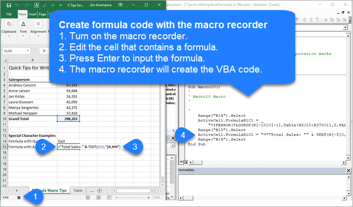
Here are the steps to creating the formula property code with the macro recorder.
- Turn on the macro recorder (Developer tab > Record Macro)
- Type your formula or edit an existing formula.
- Press Enter to enter the formula.
- The code is created in the macro.
If your formula contains quotation marks or ampersand symbols, the macro recorder will account for this. It creates all the sub-strings and wraps everything in quotes properly. Here is an example.
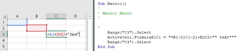
Sub Macro10()
'Use the macro recorder to create code for complex formulas with
'special characters and relative references

  ActiveCell.FormulaR1C1 = "=""Total Sales: "" & TEXT(R[-5]C,""$#,###"")"

End Sub
Tip #3: R1C1 Style Formula Notation
If you use the macro recorder for formulas, you will notices that it creates code with the FormulaR1C1 property.
R1C1 style notation allows us to create both relative (A1), absolute ($A$1), and mixed ($A1, A$1) references in our macro code.
R1C1 stands for Rows and Columns.
Relative References
For relative references we specify the number of rows and columns we want to offset from the cell that the formula is in. The number of rows and columns are referenced in square brackets.
The following would create a reference to a cell that is 3 rows above and 2 rows to the right of the cell that contains the formula.
R[-3]C[2]
Negative numbers go up rows and columns to the left.
Positive numbers go down rows and columns to the right.
Absolute References
We can also use R1C1 notation for absolute references. This would typically look like $A$2.
For absolute references we do NOT use the square brackets. The following would create a direct reference to cell $A$2, row 2 column 1
R2C1
Mixed References
with mixed references we add the square brackets for either the row or column reference, and no brackets for the other reference. The following formula in cell B2 would create this reference to A$2, where the row is absolute and the column is relative.
R2C[-1]
When creating mixed references, the relative row or column number will depend on what cell the formula is in.
It’s easiest to just use the macro recorder to figure these out.
FormulaR1C1 Property versus Formula Property
The FormulaR1C1 property reads the R1C1 notation and creates the proper references in the cells. If you use the regular Formula property with R1C1 notation, then VBA will attempt to put those letters in the formula, and it will likely result in a formula error.
Therefore, use the Formula property when your code contains cell references ($A$1), the FormulaR1C1 property when you need relative references that are applied to multiple cells or dependent on where the formula is entered.
If your spreadsheet changes based on conditions outside your control, like new columns or rows of data are imported from the data source, then relative references and R1C1 style notation will probably be best.
I hope those tips help. Please leave a comment below with questions or suggestions.
|
vigor Пользователь Сообщений: 172 |
Добрый вечер.Коротко суть проблемы. |
|
Kuzmich Пользователь Сообщений: 7998 |
ActiveCell.Formula = «=SUM(ActiveSheet(«111»).Range(Cells(1,переменная), _ |
|
vigor Пользователь Сообщений: 172 |
Не работает.Сами попробуйте, я так уже експериментировал |
|
nerv  Пользователь Сообщений: 3071 |
ActiveCell.Formula = «=СУММ(» & Range(«A2»).Address & «,» & Range(«A3»).Address & «)» |
|
Hugo Пользователь Сообщений: 23251 |
Идиотская конструкция получилась… With Sheets(«111») |
|
Hugo Пользователь Сообщений: 23251 |
Лист потерялся, не заметил… ActiveCell.Formula = «=SUM(111!» & Cells(1, m).Address & «,111!» & Cells(5, n).Address & «)» |
|
Hugo Пользователь Сообщений: 23251 |
|
|
Насчет ActiveSheet(«111») согласен Prist.Спешил.Все остальное работает спасибо ребята |
|
|
vigor Пользователь Сообщений: 172 |
Ребятки посоветуйте книгу по RibbonX,или прикольную статейку в Нете.Буду благодарен |
|
nerv Пользователь Сообщений: 3071 |
Но его радость была бы не полной. Позвольте добавить идиотизма : ) ActiveCell.Formula = «=СУММ(‘» & Sheets(«111»).Name & «‘!» & Range(«A2»).Address & «,» & Range(«A3»).Address & «)» |
|
nerv Пользователь Сообщений: 3071 |
#11 02.07.2011 10:50:13 {quote}{login=The_Prist}{date=02.07.2011 09:58}{thema=Re: }{post}{quote}{login=nerv}{date=01.07.2011 11:22}{thema=}{post}Но его радость была бы не полной. Позвольте добавить идиотизма : ) ActiveCell.Formula = «=СУММ(‘» & Sheets(«111»).Name & «‘!» & Range(«A2»).Address & «,» & Range(«A3»).Address & «)»{/post}{/quote}А Вы уверены, что в таком случае суммироваться будут ячейки с одного только листа «111»? Специально заменил СУММ на SUM, т.к. в таком случае локализация не влияет и формула не выдаст ИМЯ.{/post}{/quote}не уверен Чебурашка стал символом олимпийских игр. А чего достиг ты? |

