
Свойство ActiveCell объекта Application, применяемое в VBA для возвращения активной ячейки, расположенной на активном листе в окне приложения Excel.
Свойство ActiveCell объекта Application возвращает объект Range, представляющий активную ячейку на активном листе в активном или указанном окне приложения Excel. Если окно не отображает лист, применение свойства Application.ActiveCell приведет к ошибке.
Если свойство ActiveCell применяется к активному окну приложения Excel, то идентификатор объекта (Application или ActiveWindow) можно в коде VBA Excel не указывать. Следующие выражения, скопированные с сайта разработчиков, являются эквивалентными:
|
ActiveCell Application.ActiveCell ActiveWindow.ActiveCell Application.ActiveWindow.ActiveCell |
Но если нам необходимо возвратить активную ячейку, находящуюся в неактивном окне приложения Excel, тогда без указания идентификатора объекта на обойтись:
|
Sub Primer1() With Windows(«Книга2.xlsx») .ActiveCell = 325 MsgBox .ActiveCell.Address MsgBox .ActiveCell.Value End With End Sub |
Программно сделать ячейку активной в VBA Excel можно с помощью методов Activate и Select.
Различие методов Activate и Select
Выберем программно диапазон «B2:E6» методом Select и выведем адрес активной ячейки:
|
Sub Primer2() Range(«B2:E6»).Select ActiveCell = ActiveCell.Address End Sub |
Результат:

Как видим, активной стала первая ячейка выбранного диапазона, расположенная слева вверху. Если мы поменяем местами границы диапазона (Range("E6:B2").Select), все равно активной станет та же первая ячейка.
Теперь сделаем активной ячейку «D4», расположенную внутри выделенного диапазона, с помощью метода Activate:
|
Sub Primer3() Range(«E6:B2»).Select Range(«D4»).Activate ActiveCell = ActiveCell.Address End Sub |
Результат:

Как видим, выбранный диапазон не изменился, а активная ячейка переместилась из первой ячейки выделенного диапазона в ячейку «D4».
И, наконец, выберем ячейку «D4», расположенную внутри выделенного диапазона, с помощью метода Select:
|
Sub Primer4() Range(«E6:B2»).Select Range(«D4»).Select ActiveCell = ActiveCell.Address End Sub |
Результат:

Как видим, ранее выбранный диапазон был заменен новым, состоящим из одной ячейки «D4». Такой же результат будет и при активации ячейки, расположенной вне выбранного диапазона, методом Activate:
|
Sub Primer5() Range(«E6:B2»).Select Range(«A3»).Activate ActiveCell = ActiveCell.Address End Sub |
Аналогично ведут себя методы Activate и Select при работе с выделенной группой рабочих листов.
Свойство Application.ActiveCell используется для обращения к одной ячейке, являющейся активной, а для работы со всеми ячейками выделенного диапазона используется свойство Application.Selection.
Home / VBA / How to use ActiveCell in VBA in Excel
In VBA, the active cell is a property that represents the cell that is active at the moment. When you select a cell or navigate to a cell and that green box covers that cell you can use ACTIVECELL property to refer to that cell in a VBA code. There are properties and methods that come with it.

Use the Active Cell Property
- Type the keyword “ActiveCell”.
- Type a dot (.) to get the list properties and methods.
- Select the property or method that you want to use.
- Run the code to perform the activity to the active cell.

Important Points
- When you use the active cell property VBA refers to the active cell of the active workbook’s active sheet’s, irrespective of how many workbooks are open at the moment.
- ActiveCell is ultimately a cell that comes with all the properties and methods that a normal cell comes with.
Activate a Cell from the Selected Range
To activate a cell using a VBA code there are two ways that you can use one “Activate” method and “Select” method.
Sub vba_activecell()

'select and entire range
Range("A1:A10").Select

'select the cell A3 from the selected range
Range("A3").Activate

'clears everything from the active cell
ActiveCell.Clear

End Sub
The above code, first of all, selects the range A1:A10 and then activates the cell A3 out of that and in the end, clears everything from the active cell i.e., A3.
Return Value from the Active Cell
The following code returns the value from the active cell using a message box.
MsgBox ActiveCell.ValueOr if you want to get the value from the active cell and paste it into a separate cell.
Range("A1") = ActiveCell.ValueSet Active Cell to a Variable
You can also set the active cell to the variable, just like the following example.
Sub vba_activecell()

'declares the variable as range
Dim myCell As Range

'set active cell to the variable
Set myCell = ActiveCell

'enter value in the active cell
myCell.Value = Done

End Sub
Get Row and Column Number of the ActiveCell
With the active cell there comes a row and column property that you can use to get the row and column number of the active cell.
MsgBox ActiveCell.Row

MsgBox ActiveCell.Column
Get Active Cell’s Address
You can use the address property to get the address of the active cell.
MsgBox ActiveCell.AddressWhen you run the above code, it shows you a message box with the cell address of the active cell of the active workbook’s active sheet (as I mentioned earlier).
Move from the Active Cell using Offset
With offset property, you can move to a cell which is a several rows and columns away from the active cell.
ActiveCell.Offset(2, 2).SelectSelect a Range from the Active Cell
And you can also select a range starting from the active cell.
Range(ActiveCell.Offset(1, 1), ActiveCell.Offset(5, 5)).SelectMore Tutorials
- Count Rows using VBA in Excel
- Excel VBA Font (Color, Size, Type, and Bold)
- Excel VBA Hide and Unhide a Column or a Row
- Excel VBA Range – Working with Range and Cells in VBA
- Apply Borders on a Cell using VBA in Excel
- Find Last Row, Column, and Cell using VBA in Excel
- Insert a Row using VBA in Excel
- Merge Cells in Excel using a VBA Code
- Select a Range/Cell using VBA in Excel
- SELECT ALL the Cells in a Worksheet using a VBA Code
- Special Cells Method in VBA in Excel
- UsedRange Property in VBA in Excel
- VBA AutoFit (Rows, Column, or the Entire Worksheet)
- VBA ClearContents (from a Cell, Range, or Entire Worksheet)
- VBA Copy Range to Another Sheet + Workbook
- VBA Enter Value in a Cell (Set, Get and Change)
- VBA Insert Column (Single and Multiple)
- VBA Named Range | (Static + from Selection + Dynamic)
- VBA Range Offset
- VBA Sort Range | (Descending, Multiple Columns, Sort Orientation
- VBA Wrap Text (Cell, Range, and Entire Worksheet)
- VBA Check IF a Cell is Empty + Multiple Cells
⇠ Back to What is VBA in Excel
Helpful Links – Developer Tab – Visual Basic Editor – Run a Macro – Personal Macro Workbook – Excel Macro Recorder – VBA Interview Questions – VBA Codes
‘Active Cell’ is an important concept in Excel.
While you don’t have to care about the active cell when you’re working on the worksheet, it’s an important thing to know when working with VBA in Excel.
Proper use of the active cell in Excel VBA can help you write better code.
In this tutorial, I first explained what is an active cell, and then show you some examples of how to use an active cell in VBA in Excel.
What is an Active Cell in Excel?
An active cell, as the name suggests, is the currently active cell that will be used when you enter any text or formula in Excel.
For example, if I select cell B5, then B5 becomes my active cell in the worksheet. Now if I type anything from my keyboard, it would be entered in this cell, because this is the active cell.
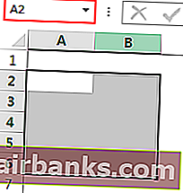
While this may sound obvious, here is something not that obvious – when you select a range of cells, even then you would only have one active cell.
For example, if I select A1:B10, although I have 20 selected cells, I still have only one single active cell.
So now, if I start typing any text or formula, it would only be entered in the active cell.
You can identify the active cell by looking at the difference in color between the active cell in all the other cells in the selection. You would notice that the active cell is of a lighter shade than the other selected cells.

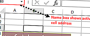
Another quick way to know which cell is the active cell is by looking at the Name box (the field that is next to the formula bar). The cell reference of the active cell would be shown in the Name Box.

Using Active Cell in VBA in Excel
Now that I’ve explained what is an active cell in a worksheet in excel, let’s learn how an Active cell can be used in Excel VBA.
Active Cell Properties and Methods
In VBA, you can use an active cell in two ways:
- To get the information about it (these are called Properties)
- To perform some action on it (these are called Methods)
Here is how you can access all the properties and methods of an active cell in VBA:
- Open a Module in Excel VBA editor
- Type the phrase ‘ActiveCell’
- Enter a dot (.) after the word ActiveCell
As soon as you do this, you would notice that a set of properties and methods appear as a drop-down (this is called an IntelliSense in Excel VBA).
In the drop-down that appears, you would see two types of options – the one that has a green icon and the one that has a gray icon (with a hand).
The one with the grey icons is the Properties, and the one with the green icons is the Methods.
Some examples of Methods would include Activate, AddComment, Cut, Delete, Clear, etc. As you can notice, these are actions that can be performed on the active cell.
Some examples of Properties would include Address, Font, HasFormula, Interior.Color. All these are properties of the active cell that gives you information about that active cell.
For example, you can use this to get the cell address of the active cell or change the interior cell color of the cell.
Now let’s have a few simple VBA code examples that you can use in your day-to-day work when working with active cell in excel
Making a Cell the Active Cell
To make any cell the active cell, you first have to make sure that it is selected.
If you only have one single cell selected, it by default becomes the active cell.
Below is the VBA code to make cell B5 the active cell:
Sub Change_ActiveCell()
Range("B5").Activate
End Sub
In the above VBA code, I have first specified the cell address of the cell that I want to activate (which is B5), and then I use the activate method to make it the active cell.
When you only want to make one single cell the active cell, you can also use the select method (code below):
Sub Change_ActiveCell()
Range("B5").Select
End Sub
As I mentioned earlier, you can only have one active cell even if you have a range of cell selected.
With VBA, you can first select a range of cells, and then make any one of those cells the active cell.
Below the VBA code that would first select range A1:B10, and then make cell A5 the active cell:
Sub Select_ActiveCell()
Range("A1:B10").Select
Range("A5").Activate
End Sub
Clear the Active Cell
Below is the VBA code that would first make cell A5 the active cell, and then clear its content (cell content as well any formatting applied to the cell).
Sub Clear_ActiveCell()
Range("A5").Activate
ActiveCell.Clear
End Sub
Note that I have shown you the above code just to show you how the clear method work with active cell. In VBA, you don’t need to always select or activate the cell to perform any method on it.
For example, you can also clear the content of cell A5 using the below code:
Sub Clear_CellB5()
Range("A5").Clear
End Sub
Get the Value from the Active Cell
Below the VBA code that could show you a message box displaying the value in the active cell:
Sub Show_ActiveCell_Value()
MsgBox ActiveCell.Value
End Sub
Similarly, you can also use a simple VBA code to show the cell address of the active cell (code below):
Sub Show_ActiveCell_Address()
MsgBox ActiveCell.Address
End Sub
The above code would show the address in absolute reference (such as $A$5).

Formating the Active Cell (Color, Border)
Below the VBA code that would make the active cell blue in color and change the font color to white.
Sub Format_ActiveCell()

'Makes the active cell blue in color
ActiveCell.Interior.Color = vbBlue

'Changes the cell font color to white
ActiveCell.Font.Color = vbWhite

End Sub
Note that I have used the inbuilt color constant (vbBlue and vbWhite). You can also use the RGB constant. For example, instead of vbRed, you can use RGB(255, 0, 0)
Offsetting From the Active Cell
VBA in Excel allows you to refer to cells relative to the position of the active cell (this is called offsetting).
For example, if my active cell is cell A1, I can use the offset property on the active cell and refer to the cell below it by specifying the position of that row corresponding to the active cell.
Let me show you an example.
Sub Offset_From_ActiveCell()

'Make cell A1 the Active Cell
Range("A1").Activate

'Goes One cell Below the Actice Cell and Enters the text Test in it
ActiveCell.Offset(1, 0).Value = "Test"

End Sub
The above code first activate cell A1 and makes it the active cell. It then uses the offset property on the active cell, to refer to the cell which is one row below it.
And in the same line in the code, I have also assigned a value “Test” to that cell which is one row below the active cell.
Let me show you another example where offsetting from the active cell could be used in a practical scenario.
Below I have a VBA code that first activates cell A1, and then uses the offset property to cover 10 cells below the active cell and enter numbers from 1 to 10 in cell A1:A10.
Sub Offset_From_ActiveCell()

'Activates cell A1
Range("A1").Activate

'Loop to go through 10 cells below the active cell and enter sequential numbers in it
For i = 1 To 10
    ActiveCell.Offset(i - 1, 0).Value = i
Next i

End Sub
The above code uses a For Next loop that runs 10 times (and each time the value of the variable ‘i’ increases by 1). And since I am also using ‘i’ in the offset property, it keeps going one cell down with each iteration.
Get ActiveCell Row or Column Number
Below the VBA code that will show you the row number of the active cell in message box:
Sub ActiveCell_RowNumber()
MsgBox ActiveCell.Row
End Sub
And the below code will show you the column number in a message box:
Sub ActiveCell_ColumnNumber()
MsgBox ActiveCell.Column
End Sub
Assign Active Cell Value to a Variable
You can also use VBA to assign the active cell to a variable. Once this is done, you can use this variable instead of the active cell in your code.
And how does this help? Good Question!
When you assign the active cell to a variable, you can continue to use this variable instead of the active cell. The benefit here is that unlike the active cell (which can change when other sheets or workbooks are activated) your variable would continue to refer to the original active cell it was assigned to.
So if you are writing a VBA code that cycles through each worksheet and activates these worksheets, while your active cell would change as new sheets are activated, the variable to which you assigned the active cell initially wouldn’t change.
Below is an example code that defines a variable ‘varcell’ and assigns the active cell to this variable.
Sub Assign_ActiveCell()
Dim varcell As Range
Set varcell = ActiveCell
MsgBox varcell.Value
End Sub
Select a Range of Cells Starting from the Active Cell
And the final thing I want to show you about using active cell in Excel VBA is to select an entire range of cells starting from the active cell.
A practical use case of this could be when you want to quickly format a set of cells in every sheet in your workbook.
Below is the VBA code that would select cells in 10 rows and 10 columns starting from the active cell:
Sub Select_from_Activecell()
Range(ActiveCell, ActiveCell.Offset(10, 10)).Select
End Sub
When we specify two cell references inside the Range property, VBA refers to the entire range covered between there two references.
For example, Range(Range(“A1”), Range(“A10”)).Select would select cell A1:A10.
Similarly, I have used it with active cell, Where the first reference is the active cell itself, and the second reference offsets the active cell by 10 rows and 10 columns.
I hope this tutorial has been useful for you in understanding how active cell works in Excel VBA.
Other Excel tutorials you may also find useful:
- Highlight the Active Row and Column in a Data Range in Excel
- 24 Useful Excel Macro Examples for VBA Beginners (Ready-to-use)
- How to Filter Cells with Bold Font Formatting in Excel (An Easy Guide)
- How to Delete Entire Row in Excel Using VBA
- Copy and Paste Multiple Cells in Excel (Adjacent & Non-Adjacent)
- Working with Worksheets using Excel VBA (Explained with Examples)
- Using Workbook Object in Excel VBA (Open, Close, Save, Set)
- Excel VBA Events – An Easy (and Complete) Guide
- How to Edit Cells in Excel? (Shortcuts)
Active Cell in Excel VBA
The active cell is the currently selected cell in a worksheet. The active cell in VBA can be used as a reference to move to another cell or change the properties of the same active cell or the cell reference provided by the active cell. We can access an active cell in VBA by using the application.property method with the keyword active cell.
Understanding the concept of range object and cell properties in VBACells are cells of the worksheet, and in VBA, when we refer to cells as a range property, we refer to the same cells. In VBA concepts, cells are also the same, no different from normal excel cells.read more is important to work efficiently with VBA codingVBA code refers to a set of instructions written by the user in the Visual Basic Applications programming language on a Visual Basic Editor (VBE) to perform a specific task.read more. One more concept you need to look into in these concepts is “VBA Active Cell.”
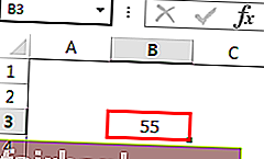
In Excel, there are millions of cells, and you are unsure which one is an active cell. For example, look at the below image.

In the above pic, we have many cells. Finding which one is an active cell is very simple; whichever cell is selected. It is called an “active cell” in VBA.
Look at the name boxIn Excel, the name box is located on the left side of the window and is used to give a name to a table or a cell. The name is usually the row character followed by the column number, such as cell A1.read more if your active cell is not visible in your window. It will show you the active cell address. For example, in the above image, the active cell address is B3.
Even when many cells are selected as a range of cells, whatever the first cell is in, the selection becomes the active cell. For example, look at the below image.

Table of contents
- Active Cell in Excel VBA
- #1 – Referencing in Excel VBA
- #2 – Active Cell Address, Value, Row, and Column Number
- #3 – Parameters of Active Cell in Excel VBA
- Recommended Articles
#1 – Referencing in Excel VBA
In our earlier articles, we have seen how to reference the cellsCell reference in excel is referring the other cells to a cell to use its values or properties. For instance, if we have data in cell A2 and want to use that in cell A1, use =A2 in cell A1, and this will copy the A2 value in A1.read more in VBA. By active cell property, we can refer to the cell.
For example, if we want to select cell A1 and insert the value “Hello,” we can write it in two ways. Below is the way of selecting the cell and inserting the value using the VBA “RANGE” object
Code:
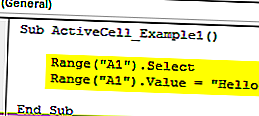
Sub ActiveCell_Example1()

    Range("A1").Select
    Range("A1").Value = "Hello"

End Sub

It will first select the cell A1 “Range(“A1″). Select”
Then, it will insert the value “Hello” in cell A1 Range(“A1”).Value = “Hello”
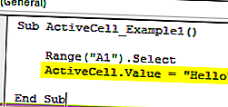
Now, we will remove the line Range(“A1”). Value = “Hello” and use the active cell property to insert the value.
Code:
Sub ActiveCell_Example1()

    Range("A1").Select
    ActiveCell.Value = "Hello"

End Sub

Similarly, first, it will select the cell A1 “Range(“A1”). Select.“
But here, we have used ActiveCell.Value = “Hello” instead of Range(“A1”).Value = “Hello”
We have used the active cell property because the moment we select cell A1 it becomes an active cell. So, we can use the Excel VBA active cell property to insert the value.
#2 – Active Cell Address, Value, Row, and Column Number
Let’s show the active cell’s address in the message box to understand it better. Now, look at the below image.

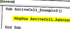
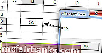
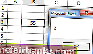
In the above image, the active cell is “B3,” and the value is 55. So, let us write code in VBA to get the active cell’s address.
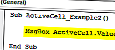
Code:
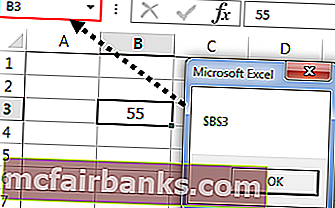
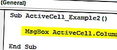
Sub ActiveCell_Example2()

    MsgBox ActiveCell.Address

End Sub

Run this code using the F5 key or manually. Then, it will show the active cell’s address in a message box.
Output:

Similarly, the below code will show the value of the active cell.
Code:
Sub ActiveCell_Example2()

    MsgBox ActiveCell.Value

End Sub

Output:

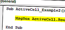
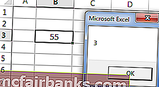
The below code will show the row number of the active cell.
Code:
Sub ActiveCell_Example2()

  MsgBox ActiveCell.Row

End Sub

Output:

The below code will show the column number of the active cell.
Code:
Sub ActiveCell_Example2()

MsgBox ActiveCell.Column

End Sub

Output:

#3 – Parameters of Active Cell in Excel VBA
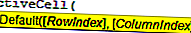
The active cell property has parameters as well. After entering the property, the active cell opens parenthesis to see the parameters.
![]()
Using this parameter, we can refer to another cell as well.
For example, ActiveCell (1,1) means whichever cell is active. If you want to move down one row to the bottom, you can use ActiveCell (2,1). Here 2 does not mean moving down two rows but rather just one row down. Similarly, if you want to move one column to the right, then this is the code ActiveCell (2,2)
Look at the below image.

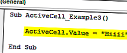
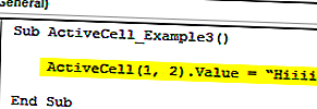
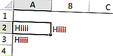
In the above image, the active cell is A2. To insert value to the active cell, you write this code.
Code:
ActiveCell.Value = “Hiiii” or ActiveCell (1,1).Value = “Hiiii”

Run this code manually or through the F5 key. It will insert the value “Hiiii” into the cell.

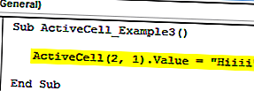
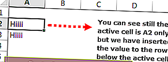
If you want to insert the same value to the below cell, you can use this code.
Code:
ActiveCell (2,1).Value = “Hiiii”

It will insert the value to the cell below the active cell.

You can use this code if you want to insert the value to one column right then.
Code:
ActiveCell (1,2).Value = “Hiiii”

It will insert “Hiiii” to the next column cell of the active cell.

Like this, we can reference the cells in VBA using the active cell property.
We hope you have enjoyed it. Thanks for your time with us.
You can download the VBA Active Cell Excel Template here:- VBA Active Cell Template
Recommended Articles
This article has been a guide to VBA Active Cell. Here, we learned the concept of an active cell to find the address of a cell. Also, we learned the parameters of the active cell in Excel VBA along with practical examples and a downloadable template. Below you can find some useful Excel VBA articles: –
- VBA Selection
- Excel Edit Cell Shortcut
- Excel VBA Range Cells
- Get Cell Value with Excel VBA
Return to VBA Code Examples
This tutorial will demonstrate how to set (and work with) the ActiveCell using VBA.
The ActiveCell property in VBA returns the address of the cell that is selected (active) in your worksheet. We can move the cell pointer to a specific cell using VBA by setting the ActiveCell property to a specific cell, and we can also read the values of the currently active cell with VBA.
Set ActiveCell
Setting the active cell in VBA is very simple – you just refer to a range as the active cell.
Sub Macro1()
   ActiveCell = Range("F2")
End Sub
This will move your cell pointer to cell F2.
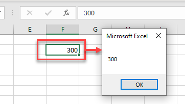
Get Value of ActiveCell
We can get the value of an active cell by populating a variable.
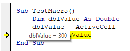
For example, if the value in F2 if 300, we can return this value to a declared variable.
Sub TestMacro()
 Dim dblValue As Double
 dblValue = ActiveCell
 MsgBox dblValue
End Sub
when we run the code, the variable dblValue will be populated with the value in the ActiveCell.
If we then allow the code to continue, a message box will pop up with the value.
Get ActiveCell in Worksheet_Change Event
When you change any data in your worksheet, the Worksheet_Change Event is fired.
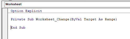
The Change event contains one argument – (ByVal Target as Range). The Range referred to in this variable Target is either a range of cells or a single cell that is currently selected in your worksheet. If you have only one cell selected in the worksheet, then the Target variable is equal to the ActiveCell.
Private Sub Worksheet_Change(ByVal Target As Range)
  If Target = Range("F2") Then
    MsgBox "The Active cell is F2!"
  End If
End Sub
Note that this event only fires when you amend the data in your worksheet – so when you add or change data, it does not fire by moving your cell pointer around the worksheet.
VBA Active Cell
Active cell means the specific cell which is active in the current active worksheet. For example, if in sheet 2 cell B4 is selected means the active cell is B4 in sheet 2. In VBA we use a reference of active cell to change the properties or values of the active cell. OR we use this function in certain situations when we need to make some changes in the active cell on some certain conditions which meet the requirements.
The active cell is a property in VBA. We use it in different situations in VBA. We can assign values to an active cell using VBA Active Cell function or fetch the address of the active cell. What did these functions return? Active cell Function returns the range property of the active cell in the active worksheet. As explained in the above statement in the definition if sheet 2 is active and cell B4 is active cell the active cell function in VBA will fetch the range properties of the cell B4 in sheet 2.
Syntax of Active Cell in Excel VBA
Below is the syntax of Active Cell in Excel VBA
The syntax is used to assign a certain value to the active cell.
Activecell.Value= “ “
The syntax will select the value or the property of the active cell in the active worksheet.
Application.Activecell
If we need to change the font of the active cell then the syntax will be as follows
Activecell.Font.(The font we want) = True
We can also display the rows and column of the active cell using the following syntax
Application.Activecell
Let us use the above syntax explained in a few examples and learn how to play with the active cells.
Note: In order to use VBA make sure to have developer’s tab enabled from File Tab from the options section.
Examples of Excel VBA Active Cell
Below are the different examples of VBA Active Cell in Excel:
You can download this VBA Active Cell Excel Template here – VBA Active Cell Excel Template
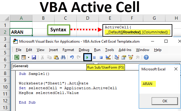
VBA Active Cell – Example #1
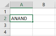
In this example, we want to change the value of the current cell with something cell. For example in sheet 1, select cell A2 and insert value as ANAND and we want to change the value for that active cell as ARAN.
Follow the below steps to use VBA Active Cell in Excel.
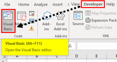
Step 1: Go to Developer’s tab and click on Visual Basic to open VB Editor.
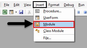
Step 2: Click on Insert tab and click on modules to insert a new module.
Step 3: Declare a sub-function to start writing the code.
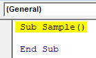
Code:
Sub Sample()

End Sub
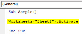
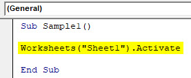
Step 4: Activate the worksheet 1 by using the below function.
Code:
Sub Sample()

Worksheets("Sheet1").Activate

End Sub
Step 5: We can check that in cell A2 in sheet 1 we have the value as ANAND and it is the active cell.
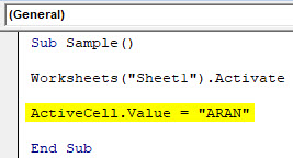
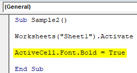
Step 6: Now use the following statement to change the value of the active cell.
Code:
Sub Sample()

Worksheets("Sheet1").Activate

ActiveCell.Value = "ARAN"

End Sub
Step 7: Run the above code from the run button provided or press F5.
We can see that the value in cell A2 has been changed.
VBA Active Cell – Example #2
Now we have changed the active cell Value from ANAND to ARAN. How do we display the current value of the active cell? This we will learn in this example.
Follow the below steps to use VBA Active Cell in Excel.
Step 1: Go to the developer’s Tab and click on Visual Basic to Open VB Editor.
Step 2: In the same module declare a sub-function to start writing the code.
Code:
Sub Sample1()

End Sub
Step 3: Activate the worksheet 1 by the following code.
Code:
Sub Sample1()

Worksheets("Sheet1").Activate

End Sub
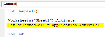
Step 4: Now let us select the active cell by the following code.
Code:
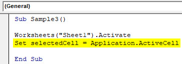
Sub Sample1()

Worksheets("Sheet1").Activate
Set selectedCell = Application.ActiveCell

End Sub
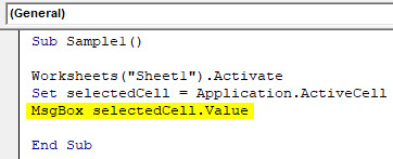
Step 5: Now let us display the value of the selected cell by the following code.
Code:
Sub Sample1()

Worksheets("Sheet1").Activate
Set selectedCell = Application.ActiveCell
MsgBox selectedCell.Value

End Sub
Step 6: Run the above code by pressing F5 or by the run button provided and see the following result.
The active cell was A2 and it has the value as ARAN so the displayed property is ARAN.
VBA Active Cell – Example #3
Let us change the font of the cell A2 which was the selected cell. Let us make the font as BOLD. Initially, there was no font selected.
For this, Follow the below steps to use VBA Active Cell in Excel.
Step 1: Go to the Developer’s Tab and click on Visual Basic to open VB Editor.
Step 2: In the same module declare a sub-function to start writing the code.
Code:
Sub Sample2()

End Sub
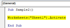
Step 3: Let us activate the worksheet first in order to use the active cell.
Code:
Sub Sample2()

Worksheets("Sheet1").Activate

End Sub
Step 4: Let us change the font of the selected cell by the following code.
Code:
Sub Sample2()

Worksheets("Sheet1").Activate

ActiveCell.Font.Bold = True

End Sub
Step 5: Run the above code by pressing F5 or by the run button provided and see the result.
The font of the active cell is changed to BOLD.
VBA Active Cell – Example #4
Now we want to know what row or what column the currently active cell is in. How to do this is what we will learn in this example.
For this, Follow the below steps to use VBA Active Cell in Excel.
Step 1: Go to Developer’s Tab and click on Visual Basic to Open the VB Editor.
Step 2: In the same module declare a sub-function to start writing the code.
Code:
Sub Sample3()

End Sub
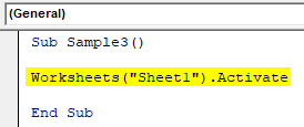
Step 3: Let us activate the worksheet first in order to use the active cell properties.
Code:
Sub Sample3()

Worksheets("Sheet1").Activate

End Sub
Step 4: Now we select the active cell by the following code.
Code:
Sub Sample3()

Worksheets("Sheet1").Activate
Set selectedCell = Application.ActiveCell

End Sub
Step 5: Now we can display the current row of the active cell by the following code.
Code:
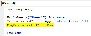
Sub Sample3()

Worksheets("Sheet1").Activate
Set selectedCell = Application.ActiveCell
MsgBox selectedCell.Row

End Sub
Step 6: We can also get the current column of the active cell by the following code.
Code:
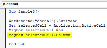
Sub Sample3()

Worksheets("Sheet1").Activate
Set selectedCell = Application.ActiveCell
MsgBox selectedCell.Row
MsgBox selectedCell.Column

End Sub
Step 7: Now press F5 or the run button provided to run the above code and see the following result.
The above result was the row of the active cell. Press ok to see the column of the active cell.
Things to Remember
There are few things which we need to remember about Active cell in VBA:
- The active cell is the currently active or selected cell in any worksheet.
- We can display or change the properties of the active cell address in VBA.
- In order to use the properties of the active cell, we must need to activate the current worksheet first.
Recommended Articles
This has been a guide to Excel VBA Active Cell. Here we discussed how to use VBA Active Cell property to assign value or fetch the address of the active cell in Excel along with some practical examples and downloadable excel template. You can also go through our other suggested articles –
- VBA IFError
- VBA XML
- VBA Paste
- VBA RGB
Активная ячейка в Excel VBA
Активная ячейка — это текущая выбранная ячейка на листе, активная ячейка в VBA может использоваться как ссылка для перехода к другой ячейке или изменения свойств той же активной ячейки или ссылки на ячейки, предоставленной из активной ячейки, активная ячейка в VBA может можно получить с помощью метода application.property с ключевым словом active cell.
Для эффективной работы с кодированием VBA важно понимать концепцию объекта диапазона и свойств ячеек в VBA. В этих концепциях есть еще одна концепция, которую вам нужно изучить, это «активная ячейка VBA».
В Excel есть миллионы ячеек, и вы наверняка сомневаетесь, какая из них является активной. Для примера посмотрите на изображение ниже.
На самом изображении выше у нас есть много ячеек, чтобы определить, какая из них является активной ячейкой, очень просто, какая бы ячейка не была выбрана прямо сейчас, она называется «Активная ячейка» в VBA.
Если ваша активная ячейка не видна в вашем окне, посмотрите на поле имени, оно покажет вам адрес активной ячейки, на приведенном выше изображении адрес активной ячейки — B3.
Даже когда в качестве диапазона ячеек выбрано множество ячеек, любая первая ячейка в выделении становится активной ячейкой. Например, посмотрите на изображение ниже.
# 1 — Ссылки в Excel VBA
В наших предыдущих статьях мы видели, как ссылаться на ячейки в VBA. По свойству Active Cell мы можем ссылаться на ячейку.
Например, если мы хотим выбрать ячейку A1 и вставить значение «Hello», мы можем записать его двумя способами. Ниже приведен способ выбора ячейки и вставки значения с помощью объекта VBA «RANGE».
Код:
Sub ActiveCell_Example1 () Диапазон ("A1"). Выберите диапазон ("A1"). Value = "Hello" End Sub
Сначала будет выбрана ячейка A1 « Диапазон (« A1 »). Выбрать»
Затем он вставит значение «Hello» в диапазон ячейки A1 («A1»). Value = «Hello»
Теперь я удалю строку Range («A1»). Value = «Hello» и использую свойство Active Cell для вставки значения.
Код:
Sub ActiveCell_Example1 () Диапазон ("A1"). Выберите ActiveCell.Value = "Hello" End Sub
Точно так же сначала он выберет ячейку A1 « Диапазон (« A1 »). Выбрать»
Но здесь я использовал ActiveCell.Value = «Hello» вместо Range («A1»). Value = «Hello»
Причина, по которой я использовал свойство Active Cell, потому что в тот момент, когда я выбираю ячейку A1, она становится активной ячейкой. Таким образом, мы можем использовать свойство Excel VBA Active Cell для вставки значения.
# 2 — Активный адрес ячейки, значение, строка и номер столбца
Чтобы понять это еще лучше, давайте покажем адрес активной ячейки в окне сообщения. Теперь посмотрите на изображение ниже.
На изображении выше активной ячейкой является «B3», а значение — 55. Давайте напишем код на VBA, чтобы получить адрес активной ячейки.
Код:
Sub ActiveCell_Example2 () MsgBox ActiveCell.Address End Sub
Запустите этот код с помощью клавиши F5 или вручную, тогда он покажет адрес активной ячейки в окне сообщения.
Выход:
Точно так же код ниже покажет значение активной ячейки.
Код:
Sub ActiveCell_Example2 () MsgBox ActiveCell.Value End Sub
Выход:
Код ниже покажет номер строки активной ячейки.
Код:
Sub ActiveCell_Example2 () MsgBox ActiveCell.Row End Sub
Выход:
Код ниже покажет номер столбца активной ячейки.
Код:
Подложка ActiveCell_Example2 () MsgBox ActiveCell.Column End Sub
Выход:
# 3 — Параметры активной ячейки в Excel VBA
Свойство Active Cell также имеет параметры. После ввода свойства ActiveCell откройте скобку, чтобы увидеть параметры.
Используя этот параметр, мы также можем ссылаться на другую ячейку.
Например, ActiveCell (1,1) означает, какая ячейка активна. Если вы хотите переместиться на одну строку ниже, вы можете использовать ActiveCell (2,1), здесь 2 не означает, что нужно переместиться на две строки вниз, а не только на одну строку вниз. Аналогично, если вы хотите переместить один столбец вправо, тогда это код ActiveCell (2,2)
Для примера посмотрите на изображение ниже.
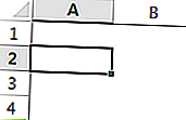
На изображении выше активной ячейкой является A2, чтобы вставить значение в активную ячейку, вы пишете этот код.
Код:
ActiveCell.Value = «Hiiii» или ActiveCell (1,1) .Value = «Hiiii»
Запустите этот код вручную или с помощью клавиши F5, это вставит значение «Hiiii» в ячейку.
Теперь, если вы хотите вставить то же значение в ячейку ниже, вы можете использовать этот код.
Код:
ActiveCell (2,1) .Value = «Hiiii»
Это вставит значение в ячейку под активной ячейкой.
Если вы хотите вставить значение в один столбец справа, вы можете использовать этот код.
Код:
ActiveCell (1,2) .Value = «Hiiii»
Это вставит «Hiiii» в следующую ячейку столбца активной ячейки.
Таким образом, мы можем ссылаться на ячейки в VBA, используя свойство Active Cell.
Надеюсь, вам понравилось. Спасибо, что уделили нам время.
Вы можете скачать шаблон VBA Active Cell Excel здесь: — VBA Active Cell Template
Всё о работе с ячейками в Excel-VBA: обращение, перебор, удаление, вставка, скрытие, смена имени.
Содержание:
Table of Contents:
- Что такое ячейка Excel?
- Способы обращения к ячейкам
- Выбор и активация
- Получение и изменение значений ячеек
- Ячейки открытой книги
- Ячейки закрытой книги
- Перебор ячеек
- Перебор в произвольном диапазоне
- Свойства и методы ячеек
- Имя ячейки
- Адрес ячейки
- Размеры ячейки
- Запуск макроса активацией ячейки
2 нюанса:
- Я почти везде стараюсь использовать ThisWorkbook (а не, например, ActiveWorkbook) для обращения к текущей книге, в которой написан этот код (считаю это наиболее безопасным для новичков способом обращения к книгам, чтобы случайно не внести изменения в другие книги). Для экспериментов можете вставлять этот код в модули, коды книги, либо листа, и он будет работать только в пределах этой книги.
- Я использую английский эксель и у меня по стандарту листы называются Sheet1, Sheet2 и т.д. Если вы работаете в русском экселе, то замените Thisworkbook.Sheets(«Sheet1») на Thisworkbook.Sheets(«Лист1»). Если этого не сделать, то вы получите ошибку в связи с тем, что пытаетесь обратиться к несуществующему объекту. Можно также заменить на Thisworkbook.Sheets(1), но это менее безопасно.
Что такое ячейка Excel?
В большинстве мест пишут: «элемент, образованный пересечением столбца и строки». Это определение полезно для людей, которые не знакомы с понятием «таблица». Для того, чтобы понять чем на самом деле является ячейка Excel, необходимо заглянуть в объектную модель Excel. При этом определения объектов «ряд», «столбец» и «ячейка» будут отличаться в зависимости от того, как мы работаем с файлом.
Объекты в Excel-VBA. Пока мы работаем в Excel без углубления в VBA определение ячейки как «пересечения» строк и столбцов нам вполне хватает, но если мы решаем как-то автоматизировать процесс в VBA, то о нём лучше забыть и просто воспринимать лист как «мешок» ячеек, с каждой из которых VBA позволяет работать как минимум тремя способами:
- по цифровым координатам (ряд, столбец),
- по адресам формата А1, B2 и т.д. (сценарий целесообразности данного способа обращения в VBA мне сложно представить)
- по уникальному имени (во втором и третьем вариантах мы будем иметь дело не совсем с ячейкой, а с объектом VBA range, который может состоять из одной или нескольких ячеек). Функции и методы объектов Cells и Range отличаются. Новичкам я бы порекомендовал работать с ячейками VBA только с помощью Cells и по их цифровым координатам и использовать Range только по необходимости.
Все три способа обращения описаны далее
Как это хранится на диске и как с этим работать вне Excel? С точки зрения хранения и обработки вне Excel и VBA. Сделать это можно, например, сменив расширение файла с .xls(x) на .zip и открыв этот архив.
Пример содержимого файла Excel:
Далее xl -> worksheets и мы видим файл листа
Содержимое файла:
То же, но более наглядно:
<?xml version="1.0" encoding="UTF-8" standalone="yes"?>
<worksheet xmlns="http://schemas.openxmlformats.org/spreadsheetml/2006/main" xmlns:r="http://schemas.openxmlformats.org/officeDocument/2006/relationships" xmlns:mc="http://schemas.openxmlformats.org/markup-compatibility/2006" mc:Ignorable="x14ac xr xr2 xr3" xmlns:x14ac="http://schemas.microsoft.com/office/spreadsheetml/2009/9/ac" xmlns:xr="http://schemas.microsoft.com/office/spreadsheetml/2014/revision" xmlns:xr2="http://schemas.microsoft.com/office/spreadsheetml/2015/revision2" xmlns:xr3="http://schemas.microsoft.com/office/spreadsheetml/2016/revision3" xr:uid="{00000000-0001-0000-0000-000000000000}">
	<dimension ref="B2:F6"/>
	<sheetViews>
		<sheetView tabSelected="1" workbookViewId="0">
			<selection activeCell="D12" sqref="D12"/>
		</sheetView>
	</sheetViews>
	<sheetFormatPr defaultRowHeight="14.4" x14ac:dyDescent="0.3"/>
	<sheetData>
		<row r="2" spans="2:6" x14ac:dyDescent="0.3">
			<c r="B2" t="s">
				<v>0</v>
			</c>
		</row>
		<row r="3" spans="2:6" x14ac:dyDescent="0.3">
			<c r="C3" t="s">
				<v>1</v>
			</c>
		</row>
		<row r="4" spans="2:6" x14ac:dyDescent="0.3">
			<c r="D4" t="s">
				<v>2</v>
			</c>
		</row>
		<row r="5" spans="2:6" x14ac:dyDescent="0.3">
			<c r="E5" t="s">
				<v>0</v></c>
		</row>
		<row r="6" spans="2:6" x14ac:dyDescent="0.3">
			<c r="F6" t="s"><v>3</v>
		</c></row>
	</sheetData>
	<pageMargins left="0.7" right="0.7" top="0.75" bottom="0.75" header="0.3" footer="0.3"/>
</worksheet>
Как мы видим, в структуре объектной модели нет никаких «пересечений». Строго говоря рабочая книга — это архив структурированных данных в формате XML. При этом в каждую «строку» входит «столбец», и в нём в свою очередь прописан номер значения данного столбца, по которому оно подтягивается из другого XML файла при открытии книги для экономии места за счёт отсутствия повторяющихся значений. Почему это важно. Если мы захотим написать какой-то обработчик таких файлов, который будет напрямую редактировать данные в этих XML, то ориентироваться надо на такую модель и структуру данных. И правильное определение будет примерно таким: ячейка — это объект внутри столбца, который в свою очередь находится внутри строки в файле xml, в котором хранятся данные о содержимом листа.
Способы обращения к ячейкам
Выбор и активация
Почти во всех случаях можно и стоит избегать использования методов Select и Activate. На это есть две причины:
- Это лишь имитация действий пользователя, которая замедляет выполнение программы. Работать с объектами книги можно напрямую без использования методов Select и Activate.
- Это усложняет код и может приводить к неожиданным последствиям. Каждый раз перед использованием Select необходимо помнить, какие ещё объекты были выбраны до этого и не забывать при необходимости снимать выбор. Либо, например, в случае использования метода Select в самом начале программы может быть выбрано два листа вместо одного потому что пользователь запустил программу, выбрав другой лист.
Можно выбирать и активировать книги, листы, ячейки, фигуры, диаграммы, срезы, таблицы и т.д.
Отменить выбор ячеек можно методом Unselect:
Selection.UnselectОтличие выбора от активации — активировать можно только один объект из раннее выбранных. Выбрать можно несколько объектов.
Если вы записали и редактируете код макроса, то лучше всего заменить Select и Activate на конструкцию With … End With. Например, предположим, что мы записали вот такой макрос:
Sub Macro1()
' Macro1 Macro
    Range("F4:F10,H6:H10").Select 'выбрали два несмежных диапазона зажав ctrl
    Range("H6").Activate          'показывает только то, что я начал выбирать второй диапазон с этой ячейки (она осталась белой). Это действие ни на что не влияет
    With Selection.Interior
        .Pattern = xlSolid
        .PatternColorIndex = xlAutomatic
        .Color = 65535            'залили желтым цветом, нажав на кнопку заливки на верхней панели
        .TintAndShade = 0
        .PatternTintAndShade = 0
    End With
End Sub
Почему макрос записался таким неэффективным образом? Потому что в каждый момент времени (в каждой строке) программа не знает, что вы будете делать дальше. Поэтому в записи выбор ячеек и действия с ними — это два отдельных действия. Этот код лучше всего оптимизировать (особенно если вы хотите скопировать его внутрь какого-нибудь цикла, который должен будет исполняться много раз и перебирать много объектов). Например, так:
Sub Macro11()
'
' Macro1 Macro
    Range("F4:F10,H6:H10").Select '1. смотрим, что за объект выбран (что идёт до .Select)
    Range("H6").Activate
    With Selection.Interior       '2. понимаем, что у выбранного объекта есть свойство interior, с которым далее идёт работа
        .Pattern = xlSolid
        .PatternColorIndex = xlAutomatic
        .Color = 65535
        .TintAndShade = 0
        .PatternTintAndShade = 0
    End With
End Sub


Sub Optimized_Macro()
    With Range("F4:F10,H6:H10").Interior '3. переносим объект напрямую в конструкцию With вместо Selection
' ////// Здесь я для надёжности прописал бы ещё Thisworkbook.Sheet("ИмяЛиста") перед Range,
' ////// чтобы минимизировать риск любых случайных изменений других листов и книг
' ////// With Thisworkbook.Sheet("ИмяЛиста").Range("F4:F10,H6:H10").Interior
        .Pattern = xlSolid               '4. полностью копируем всё, что было записано рекордером внутрь блока with
        .PatternColorIndex = xlAutomatic
        .Color = 55555                   '5. здесь я поменял цвет на зеленый, чтобы было видно, работает ли код при поочерёдном запуске двух макросов
        .TintAndShade = 0
        .PatternTintAndShade = 0
    End With
End Sub
Пример сценария, когда использование Select и Activate оправдано:
Допустим, мы хотим, чтобы во время исполнения программы мы одновременно изменяли несколько листов одним действием и пользователь видел какой-то определённый лист. Это можно сделать примерно так:
Sub Select_Activate_is_OK()
Thisworkbook.Worksheets(Array("Sheet1", "Sheet3")).Select 'Выбираем несколько листов по именам
Thisworkbook.Worksheets("Sheet3").Activate 'Показываем пользователю третий лист
'Далее все действия с выбранными ячейками через Select будут одновременно вносить изменения в оба выбранных листа

'Допустим, что тут мы решили покрасить те же два диапазона:
Range("F4:F10,H6:H10").Select
    Range("H6").Activate
    With Selection.Interior
        .Pattern = xlSolid
        .PatternColorIndex = xlAutomatic
        .Color = 65535
        .TintAndShade = 0
        .PatternTintAndShade = 0
    End With

End Sub
Единственной причиной использовать этот код по моему мнению может быть желание зачем-то показать пользователю определённую страницу книги в какой-то момент исполнения программы. С точки зрения обработки объектов, опять же, эти действия лишние.
Получение и изменение значений ячеек
Значение ячеек можно получать/изменять с помощью свойства value.
'Если нужно прочитать / записать значение ячейки, то используется свойство Value
a = ThisWorkbook.Sheets("Sheet1").Cells (1,1).Value 'записать значение ячейки А1 листа "Sheet1" в переменную "a"
ThisWorkbook.Sheets("Sheet1").Cells (1,1).Value = 1  'задать значение ячейки А1 (первый ряд, первый столбец) листа "Sheet1"

'Если нужно прочитать текст как есть (с форматированием), то можно использовать свойство .text:
ThisWorkbook.Sheets("Sheet1").Cells (1,1).Text = "1"
a = ThisWorkbook.Sheets("Sheet1").Cells (1,1).Text

'Когда проявится разница:
'Например, если мы считываем дату в формате "31 декабря 2021 г.", хранящуюся как дата
a = ThisWorkbook.Sheets("Sheet1").Cells (1,1).Value 'эапишет как "31.12.2021"
a = ThisWorkbook.Sheets("Sheet1").Cells (1,1).Text  'запишет как "31 декабря 2021 г."
Ячейки открытой книги
К ячейкам можно обращаться:
'В книге, в которой хранится макрос (на каком-то из листов, либо в отдельном модуле или форме)
ThisWorkbook.Sheets("Sheet1").Cells(1,1).Value        'По номерам строки и столбца
ThisWorkbook.Sheets("Sheet1").Cells(1,"A").Value      'По номерам строки и букве столбца
ThisWorkbook.Sheets("Sheet1").Range("A1").Value       'По адресу - вариант 1
ThisWorkbook.Sheets("Sheet1").[A1].Value              'По адресу - вариант 2
ThisWorkbook.Sheets("Sheet1").Range("CellName").Value 'По имени ячейки (для этого ей предварительно нужно его присвоить)

'Те же действия, но с использованием полного названия рабочей книги (книга должна быть открыта)
Workbooks("workbook.xlsm").Sheets("Sheet1").Cells(1,1).Value 'По номерам строки и столбца
Workbooks("workbook.xlsm").Sheets("Sheet1").Cells(1,"A").Value                'По номерам строки и букве столбца
Workbooks("workbook.xlsm").Sheets("Sheet1").Range("A1").Value                 'По адресу - вариант 1
Workbooks("workbook.xlsm").Sheets("Sheet1").[A1].Value                        'По адресу - вариант 2
Workbooks("workbook.xlsm").Sheets("Sheet1").Range("CellName").Value           'По имени ячейки (для этого ей предварительно нужно его присвоить)
Ячейки закрытой книги
Если нужно достать или изменить данные в другой закрытой книге, то необходимо прописать открытие и закрытие книги. Непосредственно работать с закрытой книгой не получится, потому что данные в ней хранятся отдельно от структуры и при открытии Excel каждый раз производит расстановку значений по соответствующим «слотам» в структуре. Подробнее о том, как хранятся данные в xlsx см выше.
Workbooks.Open Filename:="С:closed_workbook.xlsx"    'открыть книгу (она становится активной)
a = ActiveWorkbook.Sheets("Sheet1").Cells(1,1).Value  'достать значение ячейки 1,1
ActiveWorkbook.Close False                            'закрыть книгу (False => без сохранения)
Скачать пример, в котором можно посмотреть, как доставать и как записывать значения в закрытую книгу.
Код из файла:
Option Explicit
Sub get_value_from_closed_wb() 'достать значение из закрытой книги
Dim a, wb_path, wsh As String
wb_path = ThisWorkbook.Sheets("Sheet1").Cells(2, 3).Value 'get path to workbook from sheet1
wsh = ThisWorkbook.Sheets("Sheet1").Cells(3, 3).Value
Workbooks.Open Filename:=wb_path
a = ActiveWorkbook.Sheets(wsh).Cells(3, 3).Value
ActiveWorkbook.Close False
ThisWorkbook.Sheets("Sheet1").Cells(4, 3).Value = a
End Sub

Sub record_value_to_closed_wb() 'записать значение в закрытую книгу
Dim wb_path, b, wsh As String
wsh = ThisWorkbook.Sheets("Sheet1").Cells(3, 3).Value
wb_path = ThisWorkbook.Sheets("Sheet1").Cells(2, 3).Value 'get path to workbook from sheet1
b = ThisWorkbook.Sheets("Sheet1").Cells(5, 3).Value 'get value to record in the target workbook
Workbooks.Open Filename:=wb_path
ActiveWorkbook.Sheets(wsh).Cells(4, 4).Value = b 'add new value to cell D4 of the target workbook
ActiveWorkbook.Close True
End Sub
Перебор ячеек
Перебор в произвольном диапазоне
Скачать файл со всеми примерами
Пройтись по всем ячейкам в нужном диапазоне можно разными способами. Основные:
- Цикл For Each. Пример:
Sub iterate_over_cells() For Each c In ThisWorkbook.Sheets("Sheet1").Range("B2:D4").Cells MsgBox (c) Next c End SubЭтот цикл выведет в виде сообщений значения ячеек в диапазоне B2:D4 по порядку по строкам слева направо и по столбцам — сверху вниз. Данный способ можно использовать для действий, в который вам не важны номера ячеек (закрашивание, изменение форматирования, пересчёт чего-то и т.д.).
- Ту же задачу можно решить с помощью двух вложенных циклов — внешний будет перебирать ряды, а вложенный — ячейки в рядах. Этот способ я использую чаще всего, потому что он позволяет получить больше контроля над исполнением: на каждой итерации цикла нам доступны координаты ячеек. Для перебора всех ячеек на листе этим методом потребуется найти последнюю заполненную ячейку. Пример кода:
Sub iterate_over_cells() Dim cl, rw As Integer Dim x As Variant 'перебор области 3x3 For rw = 1 To 3 ' цикл для перебора рядов 1-3 For cl = 1 To 3 'цикл для перебора столбцов 1-3 x = ThisWorkbook.Sheets("Sheet1").Cells(rw + 1, cl + 1).Value MsgBox (x) Next cl Next rw 'перебор всех ячеек на листе. Последняя ячейка определена с помощью UsedRange 'LastRow = ActiveSheet.UsedRange.Row + ActiveSheet.UsedRange.Rows.Count - 1 'LastCol = ActiveSheet.UsedRange.Column + ActiveSheet.UsedRange.Columns.Count - 1 'For rw = 1 To LastRow 'цикл перебора всех рядов ' For cl = 1 To LastCol 'цикл для перебора всех столбцов ' Действия ' Next cl 'Next rw End Sub - Если нужно перебрать все ячейки в выделенном диапазоне на активном листе, то код будет выглядеть так:
Sub iterate_cell_by_cell_over_selection() Dim ActSheet As Worksheet Dim SelRange As Range Dim cell As Range Set ActSheet = ActiveSheet Set SelRange = Selection 'if we want to do it in every cell of the selected range For Each cell In Selection MsgBox (cell.Value) Next cell End SubДанный метод подходит для интерактивных макросов, которые выполняют действия над выбранными пользователем областями.
- Перебор ячеек в ряду
Sub iterate_cells_in_row() Dim i, RowNum, StartCell As Long RowNum = 3 'какой ряд StartCell = 0 ' номер начальной ячейки (минус 1, т.к. в цикле мы прибавляем i) For i = 1 To 10 ' 10 ячеек в выбранном ряду ThisWorkbook.Sheets("Sheet1").Cells(RowNum, i + StartCell).Value = i '(i + StartCell) добавляет 1 к номеру столбца при каждом повторении Next i End Sub - Перебор ячеек в столбце
Sub iterate_cells_in_column() Dim i, ColNum, StartCell As Long ColNum = 3 'какой столбец StartCell = 0 ' номер начальной ячейки (минус 1, т.к. в цикле мы прибавляем i) For i = 1 To 10 ' 10 ячеек ThisWorkbook.Sheets("Sheet1").Cells(i + StartCell, ColNum).Value = i ' (i + StartCell) добавляет 1 к номеру ряда при каждом повторении Next i End Sub
Свойства и методы ячеек
Имя ячейки
Присвоить новое имя можно так:
Thisworkbook.Sheets(1).Cells(1,1).name = "Новое_Имя"Для того, чтобы сменить имя ячейки нужно сначала удалить существующее имя, а затем присвоить новое. Удалить имя можно так:
ActiveWorkbook.Names("Старое_Имя").DeleteПример кода для переименования ячеек:
Sub rename_cell()

old_name = "Cell_Old_Name"
new_name = "Cell_New_Name"

ActiveWorkbook.Names(old_name).Delete
ThisWorkbook.Sheets(1).Cells(2, 1).Name = new_name
End Sub

Sub rename_cell_reverse()

old_name = "Cell_New_Name"
new_name = "Cell_Old_Name"

ActiveWorkbook.Names(old_name).Delete
ThisWorkbook.Sheets(1).Cells(2, 1).Name = new_name
End Sub
Адрес ячейки
Sub get_cell_address() ' вывести адрес ячейки в формате буква столбца, номер ряда
  '$A$1 style
  txt_address = ThisWorkbook.Sheets(1).Cells(3, 2).Address
  MsgBox (txt_address)
End Sub

Sub get_cell_address_R1C1()' получить адрес столбца в формате номер ряда, номер столбца
  'R1C1 style
  txt_address = ThisWorkbook.Sheets(1).Cells(3, 2).Address(ReferenceStyle:=xlR1C1)
  MsgBox (txt_address)
End Sub

  'пример функции, которая принимает 2 аргумента: название именованного диапазона и тип желаемого адреса
  '(1- тип $A$1 2- R1C1 - номер ряда, столбца)
Function get_cell_address_by_name(str As String, address_type As Integer)
  '$A$1 style
  Select Case address_type
    Case 1
      txt_address = Range(str).Address
    Case 2
      txt_address = Range(str).Address(ReferenceStyle:=xlR1C1)
    Case Else
      txt_address = "Wrong address type selected. 1,2 available"
    End Select
  get_cell_address_by_name = txt_address
End Function

'перед запуском нужно убедиться, что в книге есть диапазон с названием,
'адрес которого мы хотим получить, иначе будет ошибка
Sub test_function() 'запустите эту программу, чтобы увидеть, как работает функция
  x = get_cell_address_by_name("MyValue", 2)
  MsgBox (x)
End Sub
Размеры ячейки
Ширина и длина ячейки в VBA меняется, например, так:
Sub change_size()
Dim x, y As Integer
Dim w, h As Double

'получить координаты целевой ячейки
x = ThisWorkbook.Sheets("Sheet1").Cells(2, 2).Value
y = ThisWorkbook.Sheets("Sheet1").Cells(3, 2).Value

'получить желаемую ширину и высоту ячейки
w = ThisWorkbook.Sheets("Sheet1").Cells(6, 2).Value
h = ThisWorkbook.Sheets("Sheet1").Cells(7, 2).Value

'сменить высоту и ширину ячейки с координатами x,y
ThisWorkbook.Sheets("Sheet1").Cells(x, y).RowHeight = h
ThisWorkbook.Sheets("Sheet1").Cells(x, y).ColumnWidth = w


End Sub
Прочитать значения ширины и высоты ячеек можно двумя способами (однако результаты будут в разных единицах измерения). Если написать просто Cells(x,y).Width или Cells(x,y).Height, то будет получен результат в pt (привязка к размеру шрифта).
Sub get_size()
Dim x, y As Integer
'получить координаты ячейки, с которой мы будем работать
x = ThisWorkbook.Sheets("Sheet1").Cells(2, 2).Value
y = ThisWorkbook.Sheets("Sheet1").Cells(3, 2).Value

'получить длину и ширину выбранной ячейки в тех же единицах измерения, в которых мы их задавали
ThisWorkbook.Sheets("Sheet1").Cells(2, 6).Value = ThisWorkbook.Sheets("Sheet1").Cells(x, y).ColumnWidth
ThisWorkbook.Sheets("Sheet1").Cells(3, 6).Value = ThisWorkbook.Sheets("Sheet1").Cells(x, y).RowHeight

'получить длину и ширину с помощью свойств ячейки (только для чтения) в поинтах (pt)
ThisWorkbook.Sheets("Sheet1").Cells(7, 9).Value = ThisWorkbook.Sheets("Sheet1").Cells(x, y).Width
ThisWorkbook.Sheets("Sheet1").Cells(8, 9).Value = ThisWorkbook.Sheets("Sheet1").Cells(x, y).Height

End Sub
Скачать файл с примерами изменения и чтения размера ячеек
Запуск макроса активацией ячейки
Для запуска кода VBA при активации ячейки необходимо вставить в код листа нечто подобное:
3 важных момента, чтобы это работало:
1. Этот код должен быть вставлен в код листа (здесь контролируется диапазон D4)
2-3. Программа, ответственная за запуск кода при выборе ячейки, должна называться Worksheet_SelectionChange и должна принимать значение переменной Target, относящейся к триггеру SelectionChange. Другие доступные триггеры можно посмотреть в правом верхнем углу (2).
Скачать файл с базовым примером (как на картинке)
Скачать файл с расширенным примером (код ниже)
Option Explicit

Private Sub Worksheet_SelectionChange(ByVal Target As Range)

        ' имеем в виду, что триггер SelectionChange будет запускать эту Sub после каждого клика мышью (после каждого клика будет проверяться:
          '1. количество выделенных ячеек и
          '2. не пересекается ли выбранный диапазон с заданным в этой программе диапазоном.
        ' поэтому в эту программу не стоит без необходимости писать никаких других тяжелых операций

    If Selection.Count = 1 Then 'запускаем программу только если выбрано не более 1 ячейки


    'вариант модификации - брать адрес ячейки из другой ячейки:
    'Dim CellName as String
    'CellName = Activesheet.Cells(1,1).value 'брать текстовое имя контролируемой ячейки из A1 (должно быть в формате Буква столбца + номер строки)
    'If Not Intersect(Range(CellName), Target) Is Nothing Then
    'для работы этой модификации следующую строку надо закомментировать/удалить


        If Not Intersect(Range("D4"), Target) Is Nothing Then
        'если заданный (D4) и выбранный диапазон пересекаются
        '(пересечение диапазонов НЕ равно Nothing)

        'можно прописать диапазон из нескольких ячеек:
        'If Not Intersect(Range("D4:E10"), Target) Is Nothing Then
        'можно прописать несколько диапазонов:
        'If Not Intersect(Range("D4:E10"), Target) Is Nothing or Not Intersect(Range("A4:A10"), Target) Is Nothing Then

            Call program 'выполняем программу
        End If
    End If
End Sub

Sub program()

MsgBox ("Program Is running") 'здесь пишем код того, что произойдёт при выборе нужной ячейки


End Sub