
| title | keywords | f1_keywords | ms.prod | api_name | ms.assetid | ms.date | ms.localizationpriority |
|---|---|---|---|---|---|---|---|
|
Worksheet.Range property (Excel) |
vbaxl10.chm175120 |
vbaxl10.chm175120 |
excel |
Excel.Worksheet.Range |
9a323305-c822-ef9e-1cc8-ec077a976834 |
05/30/2019 |
medium |
Worksheet.Range property (Excel)
Returns a Range object that represents a cell or a range of cells.
Syntax
expression.Range (Cell1, Cell2)
expression A variable that represents a Worksheet object.
Parameters
| Name | Required/Optional | Data type | Description |
|---|---|---|---|
| Cell1 | Required | Variant | A String that is a range reference when one argument is used. Either a String that is a range reference or a Range object when two arguments are used. |
| Cell2 | Optional | Variant | Either a String that is a range reference or a Range object. Cell2 defines another extremity of the range returned by the property. |
Remarks
Cell1 and Cell2 can be A1-style references in the language of the macro. The range references can include the range operator (a colon), intersection operator (a space), or union operator (a comma). They can also include dollar signs, which are ignored. A local defined name can be a range reference. If you use a name, the name is assumed to be in the language of the macro.
Cell1 and Cell2 can be Range objects that contain a single cell, column, row, or any other range of cells.
Often, Cell1 and Cell2 are single cells in the upper-left and lower-right corners of the range returned.
When used without an object qualifier, this property is a shortcut for ActiveSheet.Range (it returns a range from the active sheet; if the active sheet isn’t a worksheet, the property fails).
When applied to a Range object, the property is relative to the Range object. For example, if the selection is cell C3, Selection.Range("B1") returns cell D3 because it is relative to the Range object returned by the Selection property. On the other hand, the code ActiveSheet.Range("B1") always returns cell B1.
Examples
This example sets the value of cell A1 on Sheet1 to 3.14159.
Worksheets("Sheet1").Range("A1").Value = 3.14159
This example creates a formula in cell A1 on Sheet1.
Worksheets("Sheet1").Range("A1").Formula = "=10*RAND()"
This example loops on cells A1:D10 on Sheet1 of the active workbook. If one of the cells has a value less than 0.001, the code replaces that value with 0 (zero).
For Each c in Worksheets("Sheet1").Range("A1:D10")
 If c.Value < .001 Then
 c.Value = 0
 End If
Next c
This example loops on the range named TestRange and displays the number of empty cells in the range.
numBlanks = 0
For Each c In Range("TestRange")
 If c.Value = "" Then
 numBlanks = numBlanks + 1
 End If
Next c
MsgBox "There are " & numBlanks & " empty cells in this range"
This example sets the font style in cells A1:C5 on Sheet1 of the active workbook to italic. The example uses Syntax 2 of the Range property.
With Worksheets("Sheet1")
	.Range(.Cells(1, 1), .Cells(5, 3)).Font.Italic = True
End With
This example compares the Worksheet.Range property, the Application.Union method, and the Application.Intersect method.
Range("A1:A10").Select                            'Selects cells A1 to A10.
Range(Range("A1"), Range("A10")).Select           'Selects cells A1 to A10.
 Range("A1, A10").Select                          'Selects cells A1 and A10.
Union(Range("A1"), Range("A10")).Select           'Selects cells A1 and A10.
 Range("A1:A5 A5:A10").Select                     'Selects cell A5.
Intersect(Range("A1:A5"), Range("A5:A10")).Select 'Selects cell A5.
[!includeSupport and feedback]
“It is a capital mistake to theorize before one has data”- Sir Arthur Conan Doyle
This post covers everything you need to know about using Cells and Ranges in VBA. You can read it from start to finish as it is laid out in a logical order. If you prefer you can use the table of contents below to go to a section of your choice.
Topics covered include Offset property, reading values between cells, reading values to arrays and formatting cells.
A Quick Guide to Ranges and Cells
| Function | Takes | Returns | Example | Gives |
|---|---|---|---|---|
|
Range |
cell address | multiple cells | .Range(«A1:A4») | $A$1:$A$4 |
| Cells | row, column | one cell | .Cells(1,5) | $E$1 |
| Offset | row, column | multiple cells | Range(«A1:A2») .Offset(1,2) |
$C$2:$C$3 |
| Rows | row(s) | one or more rows | .Rows(4) .Rows(«2:4») |
$4:$4 $2:$4 |
| Columns | column(s) | one or more columns | .Columns(4) .Columns(«B:D») |
$D:$D $B:$D |
Download the Code
The Webinar
If you are a member of the VBA Vault, then click on the image below to access the webinar and the associated source code.
(Note: Website members have access to the full webinar archive.)

Introduction
This is the third post dealing with the three main elements of VBA. These three elements are the Workbooks, Worksheets and Ranges/Cells. Cells are by far the most important part of Excel. Almost everything you do in Excel starts and ends with Cells.
Generally speaking, you do three main things with Cells
- Read from a cell.
- Write to a cell.
- Change the format of a cell.
Excel has a number of methods for accessing cells such as Range, Cells and Offset.These can cause confusion as they do similar things and can lead to confusion
In this post I will tackle each one, explain why you need it and when you should use it.
Let’s start with the simplest method of accessing cells – using the Range property of the worksheet.
Important Notes
I have recently updated this article so that is uses Value2.
You may be wondering what is the difference between Value, Value2 and the default:
' Value2
Range("A1").Value2 = 56

' Value
Range("A1").Value = 56

' Default uses value
Range("A1") = 56
Using Value may truncate number if the cell is formatted as currency. If you don’t use any property then the default is Value.
It is better to use Value2 as it will always return the actual cell value(see this article from Charle Williams.)
The Range Property
The worksheet has a Range property which you can use to access cells in VBA. The Range property takes the same argument that most Excel Worksheet functions take e.g. “A1”, “A3:C6” etc.
The following example shows you how to place a value in a cell using the Range property.
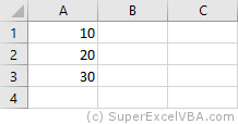
' https://excelmacromastery.com/
Public Sub WriteToCell()

    ' Write number to cell A1 in sheet1 of this workbook
    ThisWorkbook.Worksheets("Sheet1").Range("A1").Value2 = 67

    ' Write text to cell A2 in sheet1 of this workbook
    ThisWorkbook.Worksheets("Sheet1").Range("A2").Value2 = "John Smith"

    ' Write date to cell A3 in sheet1 of this workbook
    ThisWorkbook.Worksheets("Sheet1").Range("A3").Value2 = #11/21/2017#

End Sub
As you can see Range is a member of the worksheet which in turn is a member of the Workbook. This follows the same hierarchy as in Excel so should be easy to understand. To do something with Range you must first specify the workbook and worksheet it belongs to.
For the rest of this post I will use the code name to reference the worksheet.

The following code shows the above example using the code name of the worksheet i.e. Sheet1 instead of ThisWorkbook.Worksheets(“Sheet1”).
' https://excelmacromastery.com/
Public Sub UsingCodeName()

    ' Write number to cell A1 in sheet1 of this workbook
    Sheet1.Range("A1").Value2 = 67

    ' Write text to cell A2 in sheet1 of this workbook
    Sheet1.Range("A2").Value2 = "John Smith"

    ' Write date to cell A3 in sheet1 of this workbook
    Sheet1.Range("A3").Value2 = #11/21/2017#

End Sub
You can also write to multiple cells using the Range property
' https://excelmacromastery.com/
Public Sub WriteToMulti()

    ' Write number to a range of cells
    Sheet1.Range("A1:A10").Value2 = 67

    ' Write text to multiple ranges of cells
    Sheet1.Range("B2:B5,B7:B9").Value2 = "John Smith"

End Sub
You can download working examples of all the code from this post from the top of this article.
The Cells Property of the Worksheet
The worksheet object has another property called Cells which is very similar to range. There are two differences
- Cells returns a range of one cell only.
- Cells takes row and column as arguments.
The example below shows you how to write values to cells using both the Range and Cells property
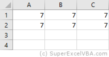
' https://excelmacromastery.com/
Public Sub UsingCells()

    ' Write to A1
    Sheet1.Range("A1").Value2 = 10
    Sheet1.Cells(1, 1).Value2  = 10

    ' Write to A10
    Sheet1.Range("A10").Value2 = 10
    Sheet1.Cells(10, 1).Value2  = 10

    ' Write to E1
    Sheet1.Range("E1").Value2 = 10
    Sheet1.Cells(1, 5).Value2  = 10

End Sub
You may be wondering when you should use Cells and when you should use Range. Using Range is useful for accessing the same cells each time the Macro runs.
For example, if you were using a Macro to calculate a total and write it to cell A10 every time then Range would be suitable for this task.
Using the Cells property is useful if you are accessing a cell based on a number that may vary. It is easier to explain this with an example.
In the following code, we ask the user to specify the column number. Using Cells gives us the flexibility to use a variable number for the column.
' https://excelmacromastery.com/
Public Sub WriteToColumn()

    Dim UserCol As Integer

    ' Get the column number from the user
    UserCol = Application.InputBox(" Please enter the column...", Type:=1)

    ' Write text to user selected column
    Sheet1.Cells(1, UserCol).Value2 = "John Smith"

End Sub
In the above example, we are using a number for the column rather than a letter.
To use Range here would require us to convert these values to the letter/number cell reference e.g. “C1”. Using the Cells property allows us to provide a row and a column number to access a cell.
Sometimes you may want to return more than one cell using row and column numbers. The next section shows you how to do this.
Using Cells and Range together
As you have seen you can only access one cell using the Cells property. If you want to return a range of cells then you can use Cells with Ranges as follows
' https://excelmacromastery.com/
Public Sub UsingCellsWithRange()

    With Sheet1
        ' Write 5 to Range A1:A10 using Cells property
        .Range(.Cells(1, 1), .Cells(10, 1)).Value2 = 5

        ' Format Range B1:Z1 to be bold
        .Range(.Cells(1, 2), .Cells(1, 26)).Font.Bold = True

    End With

End Sub
As you can see, you provide the start and end cell of the Range. Sometimes it can be tricky to see which range you are dealing with when the value are all numbers. Range has a property called Address which displays the letter/ number cell reference of any range. This can come in very handy when you are debugging or writing code for the first time.
In the following example we print out the address of the ranges we are using:
' https://excelmacromastery.com/
Public Sub ShowRangeAddress()

    ' Note: Using underscore allows you to split up lines of code
    With Sheet1

        ' Write 5 to Range A1:A10 using Cells property
        .Range(.Cells(1, 1), .Cells(10, 1)).Value2 = 5
        Debug.Print "First address is : " _
            + .Range(.Cells(1, 1), .Cells(10, 1)).Address

        ' Format Range B1:Z1 to be bold
        .Range(.Cells(1, 2), .Cells(1, 26)).Font.Bold = True
        Debug.Print "Second address is : " _
            + .Range(.Cells(1, 2), .Cells(1, 26)).Address

    End With

End Sub
In the example I used Debug.Print to print to the Immediate Window. To view this window select View->Immediate Window(or Ctrl G)


You can download all the code for this post from the top of this article.
The Offset Property of Range
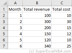
Range has a property called Offset. The term Offset refers to a count from the original position. It is used a lot in certain areas of programming. With the Offset property you can get a Range of cells the same size and a certain distance from the current range. The reason this is useful is that sometimes you may want to select a Range based on a certain condition. For example in the screenshot below there is a column for each day of the week. Given the day number(i.e. Monday=1, Tuesday=2 etc.) we need to write the value to the correct column.

We will first attempt to do this without using Offset.
' https://excelmacromastery.com/
' This sub tests with different values
Public Sub TestSelect()

    ' Monday
    SetValueSelect 1, 111.21
    ' Wednesday
    SetValueSelect 3, 456.99
    ' Friday
    SetValueSelect 5, 432.25
    ' Sunday
    SetValueSelect 7, 710.17

End Sub

' Writes the value to a column based on the day
Public Sub SetValueSelect(lDay As Long, lValue As Currency)

    Select Case lDay
        Case 1: Sheet1.Range("H3").Value2 = lValue
        Case 2: Sheet1.Range("I3").Value2 = lValue
        Case 3: Sheet1.Range("J3").Value2 = lValue
        Case 4: Sheet1.Range("K3").Value2 = lValue
        Case 5: Sheet1.Range("L3").Value2 = lValue
        Case 6: Sheet1.Range("M3").Value2 = lValue
        Case 7: Sheet1.Range("N3").Value2 = lValue
    End Select

End Sub
As you can see in the example, we need to add a line for each possible option. This is not an ideal situation. Using the Offset Property provides a much cleaner solution
' https://excelmacromastery.com/
' This sub tests with different values
Public Sub TestOffset()

    DayOffSet 1, 111.01
    DayOffSet 3, 456.99
    DayOffSet 5, 432.25
    DayOffSet 7, 710.17

End Sub

Public Sub DayOffSet(lDay As Long, lValue As Currency)

    ' We use the day value with offset specify the correct column
    Sheet1.Range("G3").Offset(, lDay).Value2 = lValue

End Sub
As you can see this solution is much better. If the number of days in increased then we do not need to add any more code. For Offset to be useful there needs to be some kind of relationship between the positions of the cells. If the Day columns in the above example were random then we could not use Offset. We would have to use the first solution.
One thing to keep in mind is that Offset retains the size of the range. So .Range(“A1:A3”).Offset(1,1) returns the range B2:B4. Below are some more examples of using Offset
' https://excelmacromastery.com/
Public Sub UsingOffset()

    ' Write to B2 - no offset
    Sheet1.Range("B2").Offset().Value2 = "Cell B2"

    ' Write to C2 - 1 column to the right
    Sheet1.Range("B2").Offset(, 1).Value2 = "Cell C2"

    ' Write to B3 - 1 row down
    Sheet1.Range("B2").Offset(1).Value2 = "Cell B3"

    ' Write to C3 - 1 column right and 1 row down
    Sheet1.Range("B2").Offset(1, 1).Value2 = "Cell C3"

    ' Write to A1 - 1 column left and 1 row up
    Sheet1.Range("B2").Offset(-1, -1).Value2 = "Cell A1"

    ' Write to range E3:G13 - 1 column right and 1 row down
    Sheet1.Range("D2:F12").Offset(1, 1).Value2 = "Cells E3:G13"

End Sub
Using the Range CurrentRegion
CurrentRegion returns a range of all the adjacent cells to the given range.
In the screenshot below you can see the two current regions. I have added borders to make the current regions clear.

A row or column of blank cells signifies the end of a current region.
You can manually check the CurrentRegion in Excel by selecting a range and pressing Ctrl + Shift + *.
If we take any range of cells within the border and apply CurrentRegion, we will get back the range of cells in the entire area.
For example
Range(“B3”).CurrentRegion will return the range B3:D14
Range(“D14”).CurrentRegion will return the range B3:D14
Range(“C8:C9”).CurrentRegion will return the range B3:D14
and so on
How to Use
We get the CurrentRegion as follows
' Current region will return B3:D14 from above example
Dim rg As Range
Set rg = Sheet1.Range("B3").CurrentRegion
Read Data Rows Only
Read through the range from the second row i.e.skipping the header row
' Current region will return B3:D14 from above example
Dim rg As Range
Set rg = Sheet1.Range("B3").CurrentRegion

' Start at row 2 - row after header
Dim i As Long
For i = 2 To rg.Rows.Count
    ' current row, column 1 of range
    Debug.Print rg.Cells(i, 1).Value2
Next i
Remove Header
Remove header row(i.e. first row) from the range. For example if range is A1:D4 this will return A2:D4
' Current region will return B3:D14 from above example
Dim rg As Range
Set rg = Sheet1.Range("B3").CurrentRegion

' Remove Header
Set rg = rg.Resize(rg.Rows.Count - 1).Offset(1)

' Start at row 1 as no header row
Dim i As Long
For i = 1 To rg.Rows.Count
    ' current row, column 1 of range
    Debug.Print rg.Cells(i, 1).Value2
Next i
Using Rows and Columns as Ranges
If you want to do something with an entire Row or Column you can use the Rows or Columns property of the Worksheet. They both take one parameter which is the row or column number you wish to access
' https://excelmacromastery.com/
Public Sub UseRowAndColumns()

    ' Set the font size of column B to 9
    Sheet1.Columns(2).Font.Size = 9

    ' Set the width of columns D to F
    Sheet1.Columns("D:F").ColumnWidth = 4

    ' Set the font size of row 5 to 18
    Sheet1.Rows(5).Font.Size = 18

End Sub
Using Range in place of Worksheet
You can also use Cells, Rows and Columns as part of a Range rather than part of a Worksheet. You may have a specific need to do this but otherwise I would avoid the practice. It makes the code more complex. Simple code is your friend. It reduces the possibility of errors.
The code below will set the second column of the range to bold. As the range has only two rows the entire column is considered B1:B2
' https://excelmacromastery.com/
Public Sub UseColumnsInRange()

    ' This will set B1 and B2 to be bold
    Sheet1.Range("A1:C2").Columns(2).Font.Bold = True

End Sub
You can download all the code for this post from the top of this article.
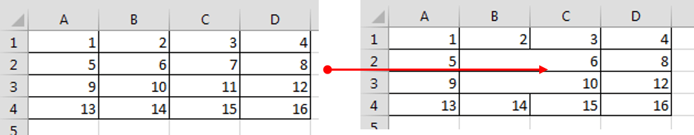
Reading Values from one Cell to another
In most of the examples so far we have written values to a cell. We do this by placing the range on the left of the equals sign and the value to place in the cell on the right. To write data from one cell to another we do the same. The destination range goes on the left and the source range goes on the right.
The following example shows you how to do this:
' https://excelmacromastery.com/
Public Sub ReadValues()

    ' Place value from B1 in A1
    Sheet1.Range("A1").Value2 = Sheet1.Range("B1").Value2

    ' Place value from B3 in sheet2 to cell A1
    Sheet1.Range("A1").Value2 = Sheet2.Range("B3").Value2

    ' Place value from B1 in cells A1 to A5
    Sheet1.Range("A1:A5").Value2 = Sheet1.Range("B1").Value2

    ' You need to use the "Value" property to read multiple cells
    Sheet1.Range("A1:A5").Value2 = Sheet1.Range("B1:B5").Value2

End Sub
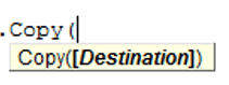
As you can see from this example it is not possible to read from multiple cells. If you want to do this you can use the Copy function of Range with the Destination parameter
' https://excelmacromastery.com/
Public Sub CopyValues()

    ' Store the copy range in a variable
    Dim rgCopy As Range
    Set rgCopy = Sheet1.Range("B1:B5")

    ' Use this to copy from more than one cell
    rgCopy.Copy Destination:=Sheet1.Range("A1:A5")

    ' You can paste to multiple destinations
    rgCopy.Copy Destination:=Sheet1.Range("A1:A5,C2:C6")

End Sub
The Copy function copies everything including the format of the cells. It is the same result as manually copying and pasting a selection. You can see more about it in the Copying and Pasting Cells section.
Using the Range.Resize Method
When copying from one range to another using assignment(i.e. the equals sign), the destination range must be the same size as the source range.
Using the Resize function allows us to resize a range to a given number of rows and columns.
For example:
' https://excelmacromastery.com/
Sub ResizeExamples()

    ' Prints A1
    Debug.Print Sheet1.Range("A1").Address

    ' Prints A1:A2
    Debug.Print Sheet1.Range("A1").Resize(2, 1).Address

    ' Prints A1:A5
    Debug.Print Sheet1.Range("A1").Resize(5, 1).Address

    ' Prints A1:D1
    Debug.Print Sheet1.Range("A1").Resize(1, 4).Address

    ' Prints A1:C3
    Debug.Print Sheet1.Range("A1").Resize(3, 3).Address

End Sub
When we want to resize our destination range we can simply use the source range size.
In other words, we use the row and column count of the source range as the parameters for resizing:
' https://excelmacromastery.com/
Sub Resize()

    Dim rgSrc As Range, rgDest As Range

    ' Get all the data in the current region
    Set rgSrc = Sheet1.Range("A1").CurrentRegion

      ' Get the range destination
    Set rgDest = Sheet2.Range("A1")
    Set rgDest = rgDest.Resize(rgSrc.Rows.Count, rgSrc.Columns.Count)

    rgDest.Value2 = rgSrc.Value2

End Sub
We can do the resize in one line if we prefer:
' https://excelmacromastery.com/
Sub ResizeOneLine()

    Dim rgSrc As Range

    ' Get all the data in the current region
    Set rgSrc = Sheet1.Range("A1").CurrentRegion

    With rgSrc
        Sheet2.Range("A1").Resize(.Rows.Count, .Columns.Count).Value2 = .Value2
    End With

End Sub
Reading Values to variables
We looked at how to read from one cell to another. You can also read from a cell to a variable. A variable is used to store values while a Macro is running. You normally do this when you want to manipulate the data before writing it somewhere. The following is a simple example using a variable. As you can see the value of the item to the right of the equals is written to the item to the left of the equals.
' https://excelmacromastery.com/
Public Sub UseVariables()

    ' Create
    Dim number As Long

    ' Read number from cell
    number = Sheet1.Range("A1").Value2

    ' Add 1 to value
    number = number + 1

    ' Write new value to cell
    Sheet1.Range("A2").Value2 = number

End Sub
To read text to a variable you use a variable of type String:
' https://excelmacromastery.com/
Public Sub UseVariableText()

    ' Declare a variable of type string
    Dim text As String

    ' Read value from cell
    text = Sheet1.Range("A1").Value2

    ' Write value to cell
    Sheet1.Range("A2").Value2 = text

End Sub
You can write a variable to a range of cells. You just specify the range on the left and the value will be written to all cells in the range.
' https://excelmacromastery.com/
Public Sub VarToMulti()

    ' Read value from cell
    Sheet1.Range("A1:B10").Value2 = 66

End Sub
You cannot read from multiple cells to a variable. However you can read to an array which is a collection of variables. We will look at doing this in the next section.
How to Copy and Paste Cells
If you want to copy and paste a range of cells then you do not need to select them. This is a common error made by new VBA users.
Note: We normally use Range.Copy when we want to copy formats, formulas, validation. If we want to copy values it is not the most efficient method.
I have written a complete guide to copying data in Excel VBA here.
You can simply copy a range of cells like this:
Range("A1:B4").Copy Destination:=Range("C5")
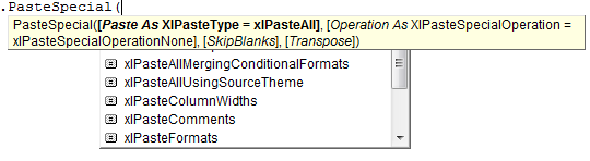
Using this method copies everything – values, formats, formulas and so on. If you want to copy individual items you can use the PasteSpecial property of range.
It works like this
Range("A1:B4").Copy
Range("F3").PasteSpecial Paste:=xlPasteValues
Range("F3").PasteSpecial Paste:=xlPasteFormats
Range("F3").PasteSpecial Paste:=xlPasteFormulas
The following table shows a full list of all the paste types
| Paste Type |
|---|
| xlPasteAll |
| xlPasteAllExceptBorders |
| xlPasteAllMergingConditionalFormats |
| xlPasteAllUsingSourceTheme |
| xlPasteColumnWidths |
| xlPasteComments |
| xlPasteFormats |
| xlPasteFormulas |
| xlPasteFormulasAndNumberFormats |
| xlPasteValidation |
| xlPasteValues |
| xlPasteValuesAndNumberFormats |
Reading a Range of Cells to an Array
You can also copy values by assigning the value of one range to another.
Range("A3:Z3").Value2 = Range("A1:Z1").Value2
The value of range in this example is considered to be a variant array. What this means is that you can easily read from a range of cells to an array. You can also write from an array to a range of cells. If you are not familiar with arrays you can check them out in this post.
The following code shows an example of using an array with a range:
' https://excelmacromastery.com/
Public Sub ReadToArray()

    ' Create dynamic array
    Dim StudentMarks() As Variant

    ' Read 26 values into array from the first row
    StudentMarks = Range("A1:Z1").Value2

    ' Do something with array here

    ' Write the 26 values to the third row
    Range("A3:Z3").Value2 = StudentMarks

End Sub
Keep in mind that the array created by the read is a 2 dimensional array. This is because a spreadsheet stores values in two dimensions i.e. rows and columns
Going through all the cells in a Range
Sometimes you may want to go through each cell one at a time to check value.
You can do this using a For Each loop shown in the following code
' https://excelmacromastery.com/
Public Sub TraversingCells()

    ' Go through each cells in the range
    Dim rg As Range
    For Each rg In Sheet1.Range("A1:A10,A20")
        ' Print address of cells that are negative
        If rg.Value < 0 Then
            Debug.Print rg.Address + " is negative."
        End If
    Next

End Sub
You can also go through consecutive Cells using the Cells property and a standard For loop.
The standard loop is more flexible about the order you use but it is slower than a For Each loop.
' https://excelmacromastery.com/
Public Sub TraverseCells()

    ' Go through cells from A1 to A10
    Dim i As Long
    For i = 1 To 10
        ' Print address of cells that are negative
        If Range("A" & i).Value < 0 Then
            Debug.Print Range("A" & i).Address + " is negative."
        End If
    Next

    ' Go through cells in reverse i.e. from A10 to A1
    For i = 10 To 1 Step -1
        ' Print address of cells that are negative
        If Range("A" & i) < 0 Then
            Debug.Print Range("A" & i).Address + " is negative."
        End If
    Next

End Sub
Formatting Cells
Sometimes you will need to format the cells the in spreadsheet. This is actually very straightforward. The following example shows you various formatting you can add to any range of cells
' https://excelmacromastery.com/
Public Sub FormattingCells()

    With Sheet1

        ' Format the font
        .Range("A1").Font.Bold = True
        .Range("A1").Font.Underline = True
        .Range("A1").Font.Color = rgbNavy

        ' Set the number format to 2 decimal places
        .Range("B2").NumberFormat = "0.00"
        ' Set the number format to a date
        .Range("C2").NumberFormat = "dd/mm/yyyy"
        ' Set the number format to general
        .Range("C3").NumberFormat = "General"
        ' Set the number format to text
        .Range("C4").NumberFormat = "Text"

        ' Set the fill color of the cell
        .Range("B3").Interior.Color = rgbSandyBrown

        ' Format the borders
        .Range("B4").Borders.LineStyle = xlDash
        .Range("B4").Borders.Color = rgbBlueViolet

    End With

End Sub
Main Points
The following is a summary of the main points
- Range returns a range of cells
- Cells returns one cells only
- You can read from one cell to another
- You can read from a range of cells to another range of cells.
- You can read values from cells to variables and vice versa.
- You can read values from ranges to arrays and vice versa
- You can use a For Each or For loop to run through every cell in a range.
- The properties Rows and Columns allow you to access a range of cells of these types
What’s Next?
Free VBA Tutorial If you are new to VBA or you want to sharpen your existing VBA skills then why not try out the The Ultimate VBA Tutorial.
Related Training: Get full access to the Excel VBA training webinars and all the tutorials.
(NOTE: Planning to build or manage a VBA Application? Learn how to build 10 Excel VBA applications from scratch.)
The VBA Range Object
The Excel Range Object is an object in Excel VBA that represents a cell, row, column, a selection of cells or a 3 dimensional range. The Excel Range is also a Worksheet property that returns a subset of its cells.
Worksheet Range
The Range is a Worksheet property which allows you to select any subset of cells, rows, columns etc.
Dim r as Range 'Declared Range variable
Set r = Range("A1") 'Range of A1 cell
Set r = Range("A1:B2") 'Square Range of 4 cells - A1,A2,B1,B2
Set r= Range(Range("A1"), Range ("B1")) 'Range of 2 cells A1 and B1
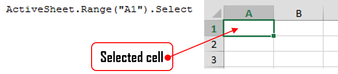
Range("A1:B2").Select 'Select the Cells A1:B2 in your Excel Worksheet
Range("A1:B2").Activate 'Activate the cells and show them on your screen (will switch to Worksheet and/or scroll to this range.
Select a cell or Range of cells using the Select method. It will be visibly marked in Excel:
Working with Range variables
The Range is a separate object variable and can be declared as other variables. As the VBA Range is an object you need to use the Set statement:
Dim myRange as Range
'...
Set myRange = Range("A1") 'Need to use Set to define myRange
The Range object defaults to your ActiveWorksheet. So beware as depending on your ActiveWorksheet the Range object will return values local to your worksheet:
Range("A1").Select
'...is the same as...
ActiveSheet.Range("A1").Select
You might want to define the Worksheet reference by Range if you want your reference values from a specifc Worksheet:
Sheets("Sheet1").Range("A1").Select 'Will always select items from Worksheet named Sheet1
The ActiveWorkbook is not same to ThisWorkbook. Same goes for the ActiveSheet. This may reference a Worksheet from within a Workbook external to the Workbook in which the macro is executed as Active references simply the currently top-most worksheet. Read more here
Range properties
The Range object contains a variety of properties with the main one being it’s Value and an the second one being its Formula.
A Range Value is the evaluated property of a cell or a range of cells. For example a cell with the formula =10+20 has an evaluated value of 20.
A Range Formula is the formula provided in the cell or range of cells. For example a cell with a formula of =10+20 will have the same Formula property.
'Let us assume A1 contains the formula "=10+20"

Debug.Print Range("A1").Value 'Returns: 30

Debug.Print Range("A1").Formula 'Returns: =10+20
Other Range properties include:
Work in progress
Worksheet Cells
A Worksheet Cells property is similar to the Range property but allows you to obtain only a SINGLE CELL, based on its row and column index. Numbering starts at 1:

The Cells property is in fact a Range object not a separate data type.
Excel facilitates a Cells function that allows you to obtain a cell from within the ActiveSheet, current top-most worksheet.
Cells(2,2).Select 'Selects B2
'...is the same as...
ActiveSheet.Cells(2,2).Select 'Select B2
Cells are Ranges which means they are not a separate data type:
Dim myRange as Range
Set myRange = Cells(1,1) 'Cell A1
Range Rows and Columns
As we all know an Excel Worksheet is divided into Rows and Columns. The Excel VBA Range object allows you to select single or multiple rows as well as single or multiple columns. There are a couple of ways to obtain Worksheet rows in VBA:
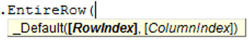
Getting an entire row or column
 To get and entire row of a specified Range you need to use the EntireRow property. Although, the function’s parameters suggest taking both a RowIndex and ColumnIndex it is enough just to provide the row number. Row indexing starts at 1.
 To get and entire column of a specified Range you need to use the EntireColumn property. Although, the function’s parameters suggest taking both a RowIndex and ColumnIndex it is enough just to provide the column number. Column indexing starts at 1.
Range("B2").EntireRows(1).Hidden = True 'Gets and hides the entire row 2

Range("B2").EntireColumns(1).Hidden = True 'Gets and hides the entire column 2
The three properties EntireRow/EntireColumn, Rows/Columns and Row/Column are often misunderstood so read through to understand the differences.
Get a row/column of a specified range
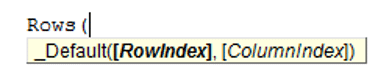 If you want to get a certain row within a Range simply use the Rows property of the Worksheet. Although, the function’s parameters suggest taking both a RowIndex and ColumnIndex it is enough just to provide the row number. Row indexing starts at 1.
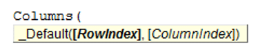 Similarly you can use the Columns function to obtain any single column within a Range. Although, the function’s parameters suggest taking both a RowIndex and ColumnIndex actually the first argument you provide will be the column index. Column indexing starts at 1.
Rows(1).Hidden = True 'Hides the first row in the ActiveSheet
'same as
ActiveSheet.Rows(1).Hidden = True

Columns(1).Hidden = True 'Hides the first column in the ActiveSheet
'same as
ActiveSheet.Columns(1).Hidden = True
To get a range of rows/columns you need to use the Range function like so:
Range(Rows(1), Rows(3)).Hidden = True 'Hides rows 1:3
'same as
Range("1:3").Hidden = True
'same as
ActiveSheet.Range("1:3").Hidden = True

Range(Columns(1), Columns(3)).Hidden = True 'Hides columns A:C
'same as
Range("A:C").Hidden = True
'same as
ActiveSheet.Range("A:C").Hidden = True
Get row/column of specified range
The above approach assumed you want to obtain only rows/columns from the ActiveSheet – the visible and top-most Worksheet. Usually however, you will want to obtain rows or columns of an existing Range. Similarly as with the Worksheet Range property, any Range facilitates the Rows and Columns property.
Dim myRange as Range
Set myRange = Range("A1:C3")

myRange.Rows.Hidden = True 'Hides rows 1:3
myRange.Columns.Hidden = True 'Hides columns A:C

Set myRange = Range("C10:F20")
myRange.Rows(2).Hidden = True 'Hides rows 11
myRange.Columns(3).Hidden = True 'Hides columns E
Getting a Ranges first row/column number
Aside from the Rows and Columns properties Ranges also facilitate a Row and Column property which provide you with the number of the Ranges first row and column.
Set myRange = Range("C10:F20")

'Get first row number
Debug.Print myRange.Row 'Result: 10
'Get first column number
Debug.Print myRange.Column 'Result: 3
Converting Column number to Excel Column
This is an often question that turns up – how to convert a column number to a string e.g. 100 to “CV”.
Function GetExcelColumn(columnNumber As Long)
    Dim div As Long, colName As String, modulo As Long
    div = columnNumber: colName = vbNullString

    Do While div > 0
        modulo = (div - 1) Mod 26
        colName = Chr(65 + modulo) & colName
        div = ((div - modulo) / 26)
    Loop

    GetExcelColumn = colName
End Function
Range Cut/Copy/Paste
Cutting and pasting rows is generally a bad practice which I heavily discourage as this is a practice that is moments can be heavily cpu-intensive and often is unaccounted for.
Copy function
 The Copy function works on a single cell, subset of cell or subset of rows/columns.
'Copy values and formatting from cell A1 to cell D1
Range("A1").Copy Range("D1")

'Copy 3x3 A1:C3 matrix to D1:F3 matrix - dimension must be same
Range("A1:C3").Copy Range("D1:F3")

'Copy rows 1:3 to rows 4:6
Range("A1:A3").EntireRow.Copy Range("A4")

'Copy columns A:C to columns D:F
Range("A1:C1").EntireColumn.Copy Range("D1")
The Copy function can also be executed without an argument. It then copies the Range to the Windows Clipboard for later Pasting.
Cut function
![]() The Cut function, similarly as the Copy function, cuts single cells, ranges of cells or rows/columns.
The Cut function, similarly as the Copy function, cuts single cells, ranges of cells or rows/columns.
'Cut A1 cell and paste it to D1
Range("A1").Cut Range("D1")

'Cut 3x3 A1:C3 matrix and paste it in D1:F3 matrix - dimension must be same
Range("A1:C3").Cut Range("D1:F3")

'Cut rows 1:3 and paste to rows 4:6
Range("A1:A3").EntireRow.Cut Range("A4")

'Cut columns A:C and paste to columns D:F
Range("A1:C1").EntireColumn.Cut Range("D1")
The Cut function can be executed without arguments. It will then cut the contents of the Range and copy it to the Windows Clipboard for pasting.
Cutting cells/rows/columns does not shift any remaining cells/rows/columns but simply leaves the cut out cells empty
PasteSpecial function
 The Range PasteSpecial function works only when preceded with either the Copy or Cut Range functions. It pastes the Range (or other data) within the Clipboard to the Range on which it was executed.
Syntax
The PasteSpecial function has the following syntax:
PasteSpecial( Paste, Operation, SkipBlanks, Transpose)
The PasteSpecial function can only be used in tandem with the Copy function (not Cut)
Parameters
Paste
The part of the Range which is to be pasted. This parameter can have the following values:
| Parameter | Constant | Description | |
|---|---|---|---|
| xlPasteSpecialOperationAdd | 2 | Copied data will be added with the value in the destination cell. | |
| xlPasteSpecialOperationDivide | 5 | Copied data will be divided with the value in the destination cell. | |
| xlPasteSpecialOperationMultiply | 4 | Copied data will be multiplied with the value in the destination cell. | |
| xlPasteSpecialOperationNone | -4142 | No calculation will be done in the paste operation. | |
| xlPasteSpecialOperationSubtract | 3 | Copied data will be subtracted with the value in the destination cell. |
Operation
The paste operation e.g. paste all, only formatting, only values, etc. This can have one of the following values:
| Name | Constant | Description |
|---|---|---|
| xlPasteAll | -4104 | Everything will be pasted. |
| xlPasteAllExceptBorders | 7 | Everything except borders will be pasted. |
| xlPasteAllMergingConditionalFormats | 14 | Everything will be pasted and conditional formats will be merged. |
| xlPasteAllUsingSourceTheme | 13 | Everything will be pasted using the source theme. |
| xlPasteColumnWidths | 8 | Copied column width is pasted. |
| xlPasteComments | -4144 | Comments are pasted. |
| xlPasteFormats | -4122 | Copied source format is pasted. |
| xlPasteFormulas | -4123 | Formulas are pasted. |
| xlPasteFormulasAndNumberFormats | 11 | Formulas and Number formats are pasted. |
| xlPasteValidation | 6 | Validations are pasted. |
| xlPasteValues | -4163 | Values are pasted. |
| xlPasteValuesAndNumberFormats | 12 | Values and Number formats are pasted. |
SkipBlanks
If True then blanks will not be pasted.
Transpose
Transpose the Range before paste (swap rows with columns).
PasteSpecial Examples
'Cut A1 cell and paste its values to D1
Range("A1").Copy
Range("D1").PasteSpecial
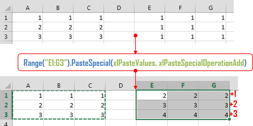
'Copy 3x3 A1:C3 matrix and add all the values to E1:G3 matrix (dimension must be same)
Range("A1:C3").Copy
Range("E1:G3").PasteSpecial xlPasteValues, xlPasteSpecialOperationAdd
Below an example where the Excel Range A1:C3 values are copied an added to the E1:G3 Range. You can also multiply, divide and run other similar operations.
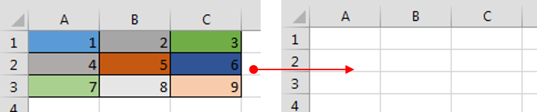
Paste
The Paste function allows you to paste data in the Clipboard to the actively selected Range. Cutting and Pasting can only be accomplished with the Paste function.
'Cut A1 cell and paste its values to D1
Range("A1").Cut
Range("D1").Select
ActiveSheet.Paste

'Cut 3x3 A1:C3 matrix and paste it in D1:F3 matrix - dimension must be same
Range("A1:C3").Cut
Range("D1:F3").Select
ActiveSheet.Paste

'Cut rows 1:3 and paste to rows 4:6
Range("A1:A3").EntireRow.Cut
Range("A4").Select
ActiveSheet.Paste

'Cut columns A:C and paste to columns D:F
Range("A1:C1").EntireColumn.Cut
Range("D1").Select
ActiveSheet.Paste
Range Clear/Delete
The Clear function
The Clear function clears the entire content and formatting from an Excel Range. It does not, however, shift (delete) the cleared cells.
Range("A1:C3").Clear
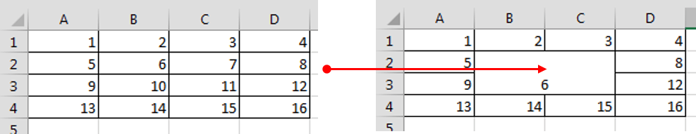
The Delete function
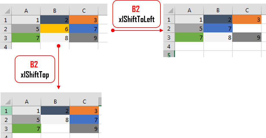
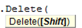 The Delete function deletes a Range of cells, removing them entirely from the Worksheet, and shifts the remaining Cells in a selected shift direction.
Although the manual Delete cell function provides 4 ways of shifting cells. The VBA Delete Shift values can only be either be xlShiftToLeft or xlShiftUp.
'If Shift omitted, Excel decides - shift up in this case
Range("B2").Delete

'Delete and Shift remaining cells left
Range("B2").Delete xlShiftToLeft

'Delete and Shift remaining cells up
Range("B2").Delete xlShiftTop

'Delete entire row 2 and shift up
Range("B2").EntireRow.Delete

'Delete entire column B and shift left
Range("B2").EntireRow.Delete
Traversing Ranges
Traversing cells is really useful when you want to run an operation on each cell within an Excel Range. Fortunately this is easily achieved in VBA using the For Each or For loops.
Dim cellRange As Range

For Each cellRange In Range("A1:C3")
  Debug.Print cellRange.Value
Next cellRange
Although this may not be obvious, beware of iterating/traversing the Excel Range using a simple For loop. For loops are not efficient on Ranges. Use a For Each loop as shown above. This is because Ranges resemble more Collections than Arrays. Read more on For vs For Each loops here
Traversing the UsedRange
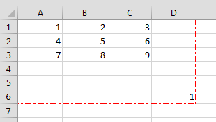 Every Worksheet has a UsedRange. This represents that smallest rectangle Range that contains all cells that have or had at some point values. In other words if the further out in the bottom, right-corner of the Worksheet there is a certain cell (e.g. E8) then the UsedRange will be as large as to include that cell starting at cell A1 (e.g. A1:E8). In Excel you can check the current UsedRange hitting CTRL+END. In VBA you get the UsedRange like this:
ActiveSheet.UsedRange
'same as
UsedRange
You can traverse through the UsedRange like this:
Dim cellRange As Range

For Each cellRange In UsedRange
  Debug.Print "Row: " & cellRange.Row & ", Column: " & cellRange.Column
Next cellRange
The UsedRange is a useful construct responsible often for bloated Excel Workbooks. Often delete unused Rows and Columns that are considered to be within the UsedRange can result in significantly reducing your file size. Read also more on the XSLB file format here
Range Addresses
The Excel Range Address property provides a string value representing the Address of the Range.
![]()
Syntax
Below the syntax of the Excel Range Address property:
Address( [RowAbsolute], [ColumnAbsolute], [ReferenceStyle], [External], [RelativeTo] )
Parameters
RowAbsolute
Optional. If True returns the row part of the reference address as an absolute reference. By default this is True.
$D$10:$G$100 'RowAbsolute is set to True
$D10:$G100 'RowAbsolute is set to False
ColumnAbsolute
Optional. If True returns the column part of the reference as an absolute reference. By default this is True.
$D$10:$G$100 'ColumnAbsolute is set to True
D$10:G$100 'ColumnAbsolute is set to False
ReferenceStyle
Optional. The reference style. The default value is xlA1. Possible values:
| Constant | Value | Description |
|---|---|---|
| xlA1 | 1 | Default. Use xlA1 to return an A1-style reference |
| xlR1C1 | -4150 | Use xlR1C1 to return an R1C1-style reference |
External
Optional. If True then property will return an external reference address, otherwise a local reference address will be returned. By default this is False.
$A$1 'Local
[Book1.xlsb]Sheet1!$A$1 'External
RelativeTo
Provided RowAbsolute and ColumnAbsolute are set to False, and the ReferenceStyle is set to xlR1C1, then you must include a starting point for the relative reference. This must be a Range variable to be set as the reference point.
Merged Ranges
![]() Merged cells are Ranges that consist of 2 or more adjacent cells. To Merge a collection of adjacent cells run Merge function on that Range.
Merged cells are Ranges that consist of 2 or more adjacent cells. To Merge a collection of adjacent cells run Merge function on that Range.
The Merge has only a single parameter – Across, a boolean which if True will merge cells in each row of the specified range as separate merged cells. Otherwise the whole Range will be merged. The default value is False.
Merge examples
To merge the entire Range:
'This will turn of any alerts warning that values may be lost
Application.DisplayAlerts = False

Range("B2:C3").Merge
This will result in the following:
To merge just the rows set Across to True.
'This will turn of any alerts warning that values may be lost
Application.DisplayAlerts = False

Range("B2:C3").Merge True
This will result in the following:
Remember that merged Ranges can only have a single value and formula. Hence, if you merge a group of cells with more than a single value/formula only the first value/formula will be set as the value/formula for your new merged Range
Checking if Range is merged
To check if a certain Range is merged simply use the Excel Range MergeCells property:
Range("B2:C3").Merge

Debug.Print Range("B2").MergeCells 'Result: True
The MergeArea
The MergeArea is a property of an Excel Range that represent the whole merge Range associated with the current Range. Say that $B$2:$C$3 is a merged Range – each cell within that Range (e.g. B2, C3..) will have the exact same MergedArea. See example below:
Range("B2:C3").Merge
Debug.Print Range("B2").MergeArea.Address 'Result: $B$2:$C$3
Named Ranges
Named Ranges are Ranges associated with a certain Name (string). In Excel you can find all your Named Ranges by going to Formulas->Name Manager. They are very useful when working on certain values that are used frequently through out your Workbook. Imagine that you are writing a Financial Analysis and want to use a common Discount Rate across all formulas. Just the address of the cell e.g. “A2”, won’t be self-explanatory. Why not use e.g. “DiscountRate” instead? Well you can do just that.
Creating a Named Range
Named Ranges can be created either within the scope of a Workbook or Worksheet:
Dim r as Range
'Within Workbook
Set r = ActiveWorkbook.Names.Add("NewName", Range("A1"))
'Within Worksheet
Set r = ActiveSheet.Names.Add("NewName", Range("A1"))
This gives you flexibility to use similar names across multiple Worksheets or use a single global name across the entire Workbook.
Listing all Named Ranges
You can list all Named Ranges using the Name Excel data type. Names are objects that represent a single NamedRange. See an example below of listing our two newly created NamedRanges:
Call ActiveWorkbook.Names.Add("NewName", Range("A1"))
Call ActiveSheet.Names.Add("NewName", Range("A1"))

Dim n As Name
For Each n In ActiveWorkbook.Names
  Debug.Print "Name: " & n.Name & ", Address: " & _
       n.RefersToRange.Address & ", Value: "; n.RefersToRange.Value
Next n

'Result:
'Name: Sheet1!NewName, Address: $A$1, Value:  1
'Name: NewName, Address: $A$1, Value:  1
SpecialCells
SpecialCells are a very useful Excel Range property, that allows you to select a subset of cells/Ranges within a certain Range.
Syntax
The SpecialCells property has the following syntax:
SpecialCells( Type, [Value] )
Parameters
Type
The type of cells to be returned. Possible values:
| Constant | Value | Description |
|---|---|---|
| xlCellTypeAllFormatConditions | -4172 | Cells of any format |
| xlCellTypeAllValidation | -4174 | Cells having validation criteria |
| xlCellTypeBlanks | 4 | Empty cells |
| xlCellTypeComments | -4144 | Cells containing notes |
| xlCellTypeConstants | 2 | Cells containing constants |
| xlCellTypeFormulas | -4123 | Cells containing formulas |
| xlCellTypeLastCell | 11 | The last cell in the used range |
| xlCellTypeSameFormatConditions | -4173 | Cells having the same format |
| xlCellTypeSameValidation | -4175 | Cells having the same validation criteria |
| xlCellTypeVisible | 12 | All visible cells |
Value
If Type is equal to xlCellTypeConstants or xlCellTypeFormulas this determines the types of cells to return e.g. with errors.
| Constant | Value |
|---|---|
| xlErrors | 16 |
| xlLogical | 4 |
| xlNumbers | 1 |
| xlTextValues | 2 |
SpecialCells examples
Get Excel Range with Constants
This will return only cells with constant cells within the Range C1:C3:
For Each r In Range("A1:C3").SpecialCells(xlCellTypeConstants)
  Debug.Print r.Value
Next r
Search for Excel Range with Errors
For Each r In ActiveSheet.UsedRange.SpecialCells(xlCellTypeFormulas, xlErrors)
  Debug.Print r.Address
Next r
In this Article
- Worksheet.Range Syntax
- Worksheet.Range Properties and Methods
- Select Method
- Copy and PasteSpecial Methods
- Font Property
- Borders Property
- CurrentRegion Property
- UsedRange Property
This tutorial will demonstrate how to use the Worksheet Range Property in VBA.
The Worksheet.Range Propety in VBA is used to specify a cell or group of cells in Excel. It returns the Worksheet.Range Object that represents the cell or cells and has a variety of methods available to it such as Select, Font, Copy and PasteSpecial to name but a few.
Worksheet.Range Syntax
The syntax of the Worksheet.Range Property is simply:
Worksheets("Sheetname").Range(Cell1,[Cell2])where Cell1 is required, and [Cell2] is optional.
Therefore to refer to cell A1 in sheet 1 we would type:
Worksheets("Sheet1").Range("A1")To refer to cell A1 to A4 (including cells A2 and A3) in Sheet 1, we can refer to the first cell, then use a colon, and refer to the last cell in the range.
Worksheets("Sheet1").Range("A1:A4")Alternatively, we can use the [Cell2] argument. This would also include cells A2 and A3 in the worksheet range.
Worksheets("Sheet1").Range("A1", "A4")If we want to refer to 2 cells that are non-contiguous, we can put a comma between the 2 cell addresses.
Worksheets("Sheet1").Range("A1, C1")Worksheet.Range Properties and Methods
Once we have used the Range Property of the Worksheet object to refer to our Range, we can then use a variety of properties and methods that are now available to the Range Object to control the appearance and /or behavior of the cells using VBA.
To see the Properties and Methods of the Range Object, we can type a period after we have declared our range.
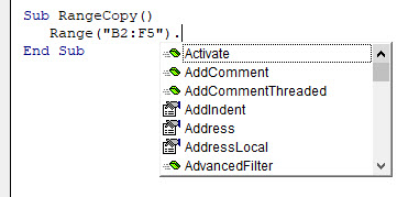
Properties will show up with the small ‘hand’ icon, while methods will show up with the small green ‘block’ icon.
Select Method
One of the most common methods to use is the select method. This enables use to select specific cells or a cell in the Excel worksheet.
To select a single cell in a worksheet, we can just refer to the single cell in the Worksheet.Range Object
Sub SelectRange
  Worksheets("Sheet1").Range("B2").Select
End Sub
To select a range of cells, we can refer to a range of cells in the Worksheet.RangeObject.
Sub SelectRange
  Worksheets("Sheet1").Range("B2:C5").Select
End Sub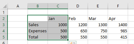
To select 2 non-contiguous ranges, we can use a comma between 2 ranges.
Sub SelectWorksheetRange
 Worksheets("Sheet1").Range("B3:B5, C2:F2").Select
End Sub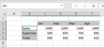
Copy and PasteSpecial Methods
We can copy the information from cells to other cells using the Copy and PasteSpecial Methods.
Sub WorksheetRangeCopy()
  Worksheets("Sheet1").Range("B2:F5").Copy
  Worksheets("Sheet1").Range("B8").PasteSpecial xlPasteAll
End Sub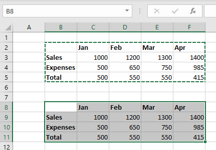
Font Property
We can use the Font Property to format the cells. In the example below, we are using the Bold property of the Font Property to bold the cells.
Sub WorksheetRangeFont()
  Worksheets("Sheet1").Range("B3:B5, C2:F2").Font.Bold = True
End Sub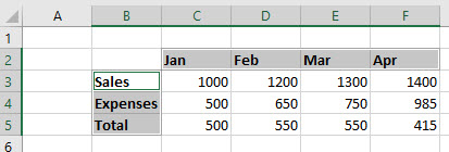
Borders Property
We can use the Borders Property, and then the LineStyle property of the Borders property to put borders around all the cells.
Sub WorksheetRangeCopy()
 Worksheets("Sheet1").Range("B2:F5").Borders.LineStyle = xlContinuous
End Sub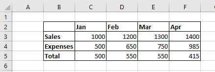
VBA Coding Made Easy
Stop searching for VBA code online. Learn more about AutoMacro — A VBA Code Builder that allows beginners to code procedures from scratch with minimal coding knowledge and with many time-saving features for all users!

Learn More
CurrentRegion Property
We can use the Current Region property of the Range object, and then the Select Method of the Current Region object to select all cells that are within the current region of the specified cell.
The current Region will select all the cells that are adjacent to the cell that is specified in the Range as long as those cells are contiguous. It will not select any cells after a blank row or column.
Sub CurrentRegion()
 Worksheets("Sheet1").Range("B2").CurrentRegion.Select
End Sub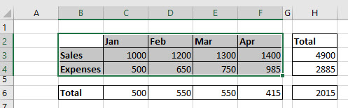
UsedRange Property
If we want to select all the cells that are populated in a worksheet, we need to use a Property of the Worksheet itself called UsedRange.
Sub UsedRangeSelect()
  Worksheets("Sheet1").UsedRange.Select
End Sub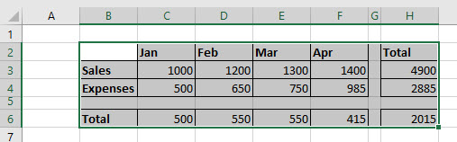
VBA Cells
The Cells keyword allows VBA to interact with cells in the worksheet.
    'Cells([row],[column])
    Cells(1,1) = 10
    Cells(2,1) = 20
    Cells(3,1) = 30
As well as entering values, we can also read values:
    VarCell = Cells(1,1)
    MsgBox VarCell
We can also perform operations, in the same way that can be done with variables:
Cells(1,3) = Cells(1,1) + Cells(2,1)
Note that the final result of the above example will be available in cell «C1» of the active worksheet.
VBA Range
Range is a command to represent intervals, containing one or more cells.
In order to establish a Range it is necessary to establish an initial cell and an end cell.
This can be done by using Cells:
    'Range([initial cell],[end cell])
    Range(Cells(1,1),Cells(2,3)) = 7
You can also set a Range from a String notation.
Range("A1:C2") = 10
In this notation, each cell is represented by a letter, referring to its column, and a number, referring to its row (E.g. «A1«). We establish with a colon : the identification of the initial cell and the end cell:
VBA Range Object
We can perform other more complex actions with Range:
Range("A1:B1").Merge 'Merge the "A1" and "B1" cells
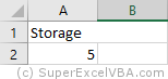
Range("A1").Value ="Storage" 'Inserts a text in "A1"
Range("A2").Formula = "=10-5" 'Inserts a formula into "A2"
Everything that comes after the dot (.) after the keyword Range is a Method or a Property.
- Method (like .Merge) is what performs an action.
- Property (like .Value) is what assigns (or has) a value or access other objects.
Throughout this tutorial we will describe the most useful Methods and Properties for the day-to-day business operations.
At the same time, everything that accepts a Method or a Property is an Object.
Therefore, we can access from the object Range the Property .Value, for example, to copy values from one range to another:
Range("C1:D3").Value = Range("A1:B3").Value
Objects, Methods, and Properties are broad concepts present in other programming languages. The study on this site will focus on the practical use in VBA.
VBA Set
Objects in VBA are only associated with variables preceded by the Set statement.
    Set Rng = Range("B2:B7")
    Rng.Value = 0 'this will set the value 0 from "B2" to "B7"
For objects there is the Object data type.
Advantages of associating a Range with a variable using Set:
- Memory loaded variables have faster processing
- Simplification of the code
VBA Range Cells
It is possible to access cells within a Range using Cells.
MsgBox Range("B2:C7").Cells(3,2) 'This will display the value of cell "C4"
Cells is a property of Range.
The Cells reference will be based on the defined Range (in this case «B2» would be equivalent to Cells(1,1)).
Worksheets Range
The Range keyword will always refer to a Worksheets. If there is no specification, it will refer to the active worksheet (ActiveSheet).
    Worksheets("Sheet1").Range("A1") 'Refers to the inactive worksheet "Sheet1"
    Range("A1") 'Refers to the active worksheet "SuperExcelVBA"
Range in this example is a property of Worksheets.
We can specify the active worksheet with .Activate method.
Worksheets("Sheet1").Activate 'Sheet1 will become the active worksheet
It is recommended to specify the worksheet whenever there is more than one in the same file.
You can explicitly reference the active worksheet by using the ActiveSheet command.
    Range("A1") = "Active Sheet"
    ActiveSheet.Range("A1") = "Active Sheet" 'Same result as above
    MsgBox ActiveSheet.Name 'Returns the name of the active sheet
You can also specify the worksheet according to its position in the file:
    Worksheets(1).Range("A1") 'Refers to the first worksheet in the order that appears in Excel ("Sheet1")
    Worksheets(2).Range("A1") 'Refers to the second worksheet in the order that appears in Excel ("SuperExcelVBA")
Thus, we can refer to the same worksheet by both ways:
    Worksheets("Sheet1").Range("A1")
    Worksheets(1).Range("A1")
Note that the first way will require changes in the code if there is a change in the name of the worksheet. In the second way, the change will be necessary if the worksheet changes position.
WorkBook Range
In the same way that a Range always refers to a Worksheet, a Worksheet always refers to a Workbook (Excel file).
Although it is common to work with only one workbook opened, referencing the Workbook is a good practice if there is an interaction with another file.
    WorkBooks("Example.xlsm").Worksheets("Sheet1").Range("A1")
    WorkBooks("Tutorial.xlsm").Worksheets("SuperExcelVBA").Range("A1")
The Worksheets in the example are a property of WorkBooks.
You need to specify both the file name and the file extension (E.g. .xlsm  ) when you use WorkBooks.
Consolidating Your Learning
Suggested Exercises
SuperExcelVBA.com is learning website. Examples might be simplified to improve reading and basic understanding. Tutorials, references, and examples are constantly reviewed to avoid errors, but we cannot warrant full correctness of all content. All Rights Reserved.
Excel ® is a registered trademark of the Microsoft Corporation.
© 2023 SuperExcelVBA | ABOUT
![]()
Хитрости »
27 Июль 2013 307022 просмотров
Полагаю не совру когда скажу, что все кто программирует в VBA очень часто в своих кодах общаются к ячейкам листов. Ведь это чуть ли не основное предназначение VBA в Excel. В принципе ничего сложного в этом нет. Например, чтобы записать в ячейку A1 слово Привет необходимо выполнить код:
Range("A1").Value = "Привет"
Тоже самое можно сделать сразу для нескольких ячеек:
Range("A1:C10").Value = "Привет"
Если необходимо обратиться к именованному диапазону:
Range("Диапазон1").Select
Диапазон1 — это имя диапазона/ячейки, к которому надо обратиться в коде. Указывается в кавычках, как и адреса ячеек.
Но в VBA есть и альтернативный метод записи значений в ячейке — через объект Cells:
Cells(1, 1).Value = "Привет"
Синтаксис объекта Range:
Range(Cell1, Cell2)
- Cell1 — первая ячейка диапазона. Может быть ссылкой на ячейку или диапазон ячеек, текстовым представлением адреса или имени диапазона/ячейки. Допускается указание несвязанных диапазонов(A1,B10), пересечений(A1 B10).
- Cell2 — последняя ячейка диапазона. Необязательна к указанию. Допускается указание ссылки на ячейку, столбец или строку.
Синтаксис объекта Cells:
Cells(Rowindex, Columnindex)
- Rowindex — номер строки
- Columnindex — номер столбца
Исходя из этого несложно предположить, что к диапазону можно обратиться, используя Cells и Range:
'выделяем диапазон "A1:B10" на активном листе
Range(Cells(1,1), Cells(10,2)).Select
и для чего? Ведь можно гораздо короче:
Иногда обращение посредством Cells куда удобнее. Например для цикла по столбцам(да еще и с шагом 3) совершенно неудобно было бы использовать буквенное обозначение столбцов.
Объект Cells так же можно использовать для указания ячеек внутри непосредственно указанного диапазона. Например, Вам необходимо выделить ячейку в 3 строке и 2 столбце диапазона «D5:F56». Можно пройтись по листу и посмотреть, отсчитать нужное количество строк и столбцов и понять, что это будет «E7». А можно сделать проще:
Range("D5:F56").Cells(3, 2).Select
Согласитесь, это гораздо удобнее, чем отсчитывать каждый раз. Особенно, если придется оперировать смещением не на 2-3 ячейки, а на 20 и более. Конечно, можно было бы применить Offset. Но данное свойство именно смещает диапазон на указанное количество строк и столбцов и придется уменьшать на 1 смещение каждого параметра для получения нужной ячейки. Да и смещает на указанное количество строк и столбцов весь диапазон, а не одну ячейку. Это, конечно, тоже не проблема — можно вдобавок к этому использовать метод Resize — но запись получится несколько длиннее и менее наглядной:
Range("D5:F56").Offset(2, 1).Resize(1, 1).Select
И неплохо бы теперь понять, как значение диапазона присвоить переменной. Для начала переменная должна быть объявлена с типом Range. А т.к. Range относится к глобальному типу Object, то присвоение значения такой переменной должно быть обязательно с применением оператора Set:
Dim rR as Range
Set rR = Range("D5")
если оператор Set не применять, то в лучшем случае получите ошибку, а в худшем(он возможен, если переменной rR не назначать тип) переменной будет назначено значение Null или значение ячейки по умолчанию. Почему это хуже? Потому что в таком случае код продолжит выполняться, но логика кода будет неверной, т.к. эта самая переменная будет содержать значение неверного типа и применение её в коде в дальнейшем все равно приведет к ошибке. Только ошибку эту отловить будет уже сложнее.
Использовать же такую переменную в дальнейшем можно так же, как и прямое обращение к диапазону:
Вроде бы на этом можно было завершить, но…Это как раз только начало. То, что я написал выше знает практически каждый, кто пишет в VBA. Основной же целью этой статьи было пояснить некоторые нюансы обращения к диапазонам. Итак, поехали.
Обычно макрорекордер при обращении к диапазону(да и любым другим объектам) сначала его выделяет, а потом уже изменяет свойство или вызывает некий метод:
'так выглядит запись слова Test в ячейку А1
Range("A1").Select
Selection.Value = "Test"
Но как правило выделение — действие лишнее. Можно записать значение и без него:
'запишем слово Test в ячейку A1 на активном листе
Range("A1").Value = "Test"
Теперь чуть подробнее разберем, как обратиться к диапазону не выделяя его и при этом сделать все правильно. Диапазон и ячейка — это объекты листа. У каждого объекта есть родитель — грубо говоря это другой объект, который является управляющим для дочернего объекта. Для ячейки родительский объект — Лист, для Листа — Книга, для Книги — Приложение Excel. Если смотреть на иерархию зависимости объектов, то от старшего к младшему получится так:
Applicaton => Workbooks => Sheets => Range
По умолчанию для всех диапазонов и ячеек родительским объектом является текущий(активный) лист. Т.е. если для диапазона(ячейки) не указать явно лист, к которому он относится, в качестве родительского листа для него будет использован текущий — ActiveSheet:
'запишем слово Test в ячейку A1 на активном листе
Range("A1").Value = "Test"
Т.е. если в данный момент активен Лист1 — то слово Test будет записано в ячейку А1 Лист1. Если активен Лист3 — в А1 Лист3. Иначе говоря такая запись равносильна записи:
ActiveSheet.Range("A1").Value = "Test"
Поэтому выхода два — либо активировать сначала нужный лист, либо записать без активации.
'активируем Лист2
Worksheets("Лист2").Select
'записываем слово Test в ячейку A1
Range("A1").Value = "Test"
Чтобы не активируя другой лист записать в него данные, необходимо явно указать принадлежность объекта Range именно этому листу:
'запишем слово Test в ячейку A1 на Лист2 независимо от того, какой лист активен
Worksheets("Лист2").Range("A1").Value = "Test"
Таким же образом происходит считывание данных с ячеек — если не указывать лист, данные ячеек которого необходимо считать — считаны будут данные с ячейки активного листа. Чтобы считать данные с Лист2 независимо от того, какой лист активен применяется такой код:
'считываем значение ячейки A1 с Лист2 независимо от того, какой лист активен
MsgBox Worksheets("Лист2").Range("A1").Value
Т.к. ячейка является частью листа, то лист в свою очередь является частью книги. Исходя из того легко сделать вывод, что при открытых двух и более книгах мы так же можем обратиться к ячейкам любого листа любой открытой книги не активируя при этом ни книгу, ни лист:
'запишем слово Test в ячейку A1 на Лист2 книги Книга2.xlsx независимо от того, какая книга и какой лист активен
Workbooks("Книга2.xlsx").Worksheets("Лист2").Range("A1").Value = "Test"
'считываем значение ячейки A1 с Лист2 книги Книга3.xlsx независимо от того, какой лист активен
MsgBox Workbooks("Книга3.xlsx").Worksheets("Лист2").Range("A1").Value
Важный момент: лучше всегда указать имя книги вместе с расширением(.xlsx, xlsm, .xls и т.д.). Если в настройках ОС Windows(Панель управления —Параметры папок -вкладка Вид —Скрывать расширения для зарегистрированных типов файлов) указано скрывать расширения — то указывать расширение не обязательно — Workbooks(«Книга2»). Но и ошибки не будет, если его указать. Однако, если пункт «Скрывать расширения для зарегистрированных типов файлов» отключен, то указание Workbooks(«Книга2») обязательно приведет к ошибке.
Очень часто ошибки обращения к ячейкам листов и книг делают начинающие, особенно в циклах по листам. Вот пример неправильного цикла:
Dim wsSh As Worksheet
For Each wsSh In ActiveWorkbook.Worksheets
    Range("A1").Value = wsSh.Name 'записываем в ячейку А1 имя листа
    MsgBox Range("A1").Value 'проверяем, то ли имя записалось
Next wsSh
MsgBox будет выдавать правильные значения, но сами имена листов будут записываться не на каждый лист, а последовательно в ячейку активного листа. Поэтому на активном листе в ячейке А1 будет имя последнего листа.
А вот так выглядит правильный цикл:
Вариант 1 — активация листа(медленный)
Dim wsSh As Worksheet
For Each wsSh In ActiveWorkbook.Worksheets
    wsSh.Activate 'активируем каждый лист
    Range("A1").Value = wsSh.Name 'записываем в ячейку А1 имя листа
    MsgBox Range("A1").Value 'проверяем, то ли имя записалось
Next wsSh
Вариант 2 — без активации листа(быстрый и более правильный)
Dim wsSh As Worksheet
For Each wsSh In ActiveWorkbook.Worksheets
    wsSh.Range("A1").Value = wsSh.Name 'записываем в ячейку А1 имя листа
    MsgBox wsSh.Range("A1").Value 'проверяем, то ли имя записалось
Next wsSh
Важно: если код записан в модуле листа(правая кнопка мыши на листе-Исходный текст) и для объекта Range или Cells родитель явно не указан(т.е. нет имени листа и книги) — тогда в качестве родителя будет использован именно тот лист, в котором записан код, независимо от того какой лист активный. Иными словами — если в модуле листа записать обращение вроде Range(«A1»).Value = «привет», то слово привет всегда будет записывать в ячейку A1 именно того листа, в котором записан сам код. Это следует учитывать, когда располагаете свои коды внутри модулей листов.
В конструкциях типа Range(Cells(,),Cells(,)) Range является контейнером, в котором указываются ссылки на объекты, из которых и будет создана ссылка на непосредственно конечный объект.
Предположим, что активен «Лист1», а код запущен с листа «Итог».
Если запись будет вида
Sheets("Итог").Range(Cells(1, 1), Cells(10, 1))
это вызовет ошибку «Run-time error ‘1004’: Application-defined or object-defined error». А ошибка появляется потому, что контейнер и объекты внутри него не могут располагаться на разных листах, равно как и:
Sheets("Итог").Range(Cells(1, 1), Sheets("Итог").Cells(10, 1))
'запись ниже так же неверна
Range(Cells(1, 1), Sheets("Итог").Cells(10, 1))
т.к. ссылки на объекты внутри контейнера относятся к разным листам. Cells(1, 1) — к активному листу, а Sheets(«Итог»).Cells(10, 1) — к листу Итог.
А вот такие записи будут правильными:
Sheets("Итог").Range(Sheets("Итог").Cells(1, 1), Sheets("Итог").Cells(10, 1))
Range(Sheets("Итог").Cells(1, 1), Sheets("Итог").Cells(10, 1))
Вторая запись не содержит ссылки на родителя для Range, но ошибки это в большинстве случаев не вызовет — т.к. если для контейнера ссылка не указана, а для двух объектов внутри контейнера родитель один — он будет применен и для самого контейнера. Однако лучше делать как в первой строке — т.е. с обязательным указанием родителя для контейнера и для его составляющих. Т.к. при определенных обстоятельствах(например, если в момент обращения к диапазону активной является книга, открытая в режиме защищенного просмотра) обращение к Range без родителя может вызывать ошибку выполнения.
Если запись будет вида Range(«A1″,»A10»), то указывать ссылку на родителя внутри Range не обязательно — достаточно будет указать эту ссылку перед самим Range — Sheets(«Итог»).Range(«A1″,»A10»), т.к. текстовое представление адреса внутри Range не является объектом(у которого может быть какой-то родительский объект), что обязывает создать ссылку именно на родителя контейнера.
Разберем пример, приближенный к жизненной ситуации. Необходимо на лист Итог занести формулу вычитания, начиная с ячейки А2 и до последней заполненной. На момент записи активен Лист1. Очень часто начинающие записывают так:
Sheets("Итог").Range("A2:A" & Cells(Rows.Count, 1).End(xlUp).Row) _
                                        .FormulaR1C1 = "=RC2-RC11"
Запись смешанная — и текстовое представление адреса ячейки(«A2:A») и ссылка на объект Cells. В данном случае явную ошибку код не вызовет, но и работать будет не всегда так, как хотелось бы. А это самое плохое, что может случиться при разработке.
Sheets(«Итог»).Range(«A2:A» — создается ссылка на столбец "A" листа Итог. Но далее идет вычисление последней строки первого столбца. И вот как раз это вычисление происходит на основе объекта Cells, который не содержит в себе ссылки на родительский объект. А значит он будет вычислять последнюю строку исключительно для текущего листа(если код записан в стандартном модуле, а не модуле листа) — т.е. для Лист1. Правильно было бы записать так:
Sheets("Итог").Range("A2:A" & Sheets("Итог").Cells(Rows.Count, 1).End(xlUp).Row) _
                                                      .FormulaR1C1 = "=RC2-RC11"
Но и здесь неверное обращение с диапазоном может сыграть злую шутку. Например, надо получить последнюю заполненную ячейку в конкретной книге:
lLastRow = Workbooks("Книга3.xls").Sheets("Лист1").Cells(Rows.Count, 1).End(xlUp).Row
с виду все нормально, но есть нюанс. Rows.Count по умолчанию будет относится к активной книге, если записано в стандартном модуле. Приведенный выше код должен работать с книгой формата 97-2003 и вычислить последнюю заполненную ячейку на листе1. В книгах формата Excel 97-2003(.xls) всего 65536 строк. Если в момент выполнения приведенной строки активна книга формата 2007 и выше(форматы .xlsx, .xlsm, .xlsb и пр) — то Rows.Count вернет 1048576, т.к. именно такое количество строк в листах книг версий Excel, начиная с 2007. И т.к. в книге, в которой мы пытаемся вычислить последнюю строку всего 65536 строк — получим ошибку 1004, т.к. не может быть номера строки 1048576 на листе с количеством строк 65536. Поэтому имеет смысл указывать явно откуда считывать Rows.Count:
lLastRow = Workbooks("Книга3.xls").Sheets("Лист1").Cells(Workbooks("Книга3.xls").Sheets("Лист1").Rows.Count, 1).End(xlUp).Row
или применить конструкцию With
With Workbooks("Книга3.xls").Sheets("Лист1")
    lLastRow = .Cells(.Rows.Count, 1).End(xlUp).Row
End With
Также не мешало бы упомянуть возможность выделения несмежного диапазона(часто его называют «рваным»). Это диапазон, который обычно привыкли выделять на листе при помощи зажатой клавиши Ctrl. Что это дает? Это дает возможность выделить одновременно ячейки A1 и B10 и записать значения только в них. Для этого есть несколько способов. Самый очевидный и описанный в справке — метод Union:
Union(Range("A1"), Range("B10")).Value = "Привет"
Однако существует и другой метод:
Range("A1,B10").Value = "Привет"
В чем отличие(я бы даже сказал преимущество) Union: можно применять в цикле по условию. Например, выделить в диапазоне A1:F50 только те ячейки, значение которых больше 10 и меньше 20:
Sub SelOne()
    Dim rCell As Range, rSel As Range
    For Each rCell In Range("A1:F50")
        If rCell.Value > 10 And rCell.Value < 20 Then
            If rSel Is Nothing Then
                Set rSel = rCell
            Else
                Set rSel = Union(rSel, rCell)
            End If
        End If
    Next rCell
    If Not rSel Is Nothing Then rSel.Select
End Sub
Конечно, можно и просто в Range через запятую передать все эти ячейки, сформировав предварительно строку. Но в случае со строкой действует ограничение: длина строки не должна превышать 255 символов.
Надеюсь, что после прочтения данной статьи проблем с обращением к диапазонам и ячейкам у Вас будет гораздо меньше.
Также см.:
Как определить последнюю ячейку на листе через VBA?
Как определить первую заполненную ячейку на листе?
Как из Excel обратиться к другому приложению
Статья помогла? Поделись ссылкой с друзьями!
![]() Видеоуроки
Видеоуроки
Поиск по меткам
Access
apple watch
Multex
Power Query и Power BI
VBA управление кодами
Бесплатные надстройки
Дата и время
Записки
ИП
Надстройки
Печать
Политика Конфиденциальности
Почта
Программы
Работа с приложениями
Разработка приложений
Росстат
Тренинги и вебинары
Финансовые
Форматирование
Функции Excel
акции MulTEx
ссылки
статистика
Присвоение диапазона ячеек объектной переменной в VBA Excel. Адресация ячеек в переменной диапазона и работа с ними. Определение размера диапазона. Примеры.
Присвоение диапазона ячеек переменной
Чтобы переменной присвоить диапазон ячеек, она должна быть объявлена как Variant, Object или Range:
|
Dim myRange1 As Variant Dim myRange2 As Object Dim myRange3 As Range |
Чтобы было понятнее, для чего переменная создана, объявляйте ее как Range.
Присваивается переменной диапазон ячеек с помощью оператора Set:
|
Set myRange1 = Range(«B5:E16») Set myRange2 = Range(Cells(3, 4), Cells(26, 18)) Set myRange3 = Selection |
В выражении Range(Cells(3, 4), Cells(26, 18)) вместо чисел можно использовать переменные.
Для присвоения диапазона ячеек переменной можно использовать встроенное диалоговое окно Application.InputBox, которое позволяет выбрать диапазон на рабочем листе для дальнейшей работы с ним.
Адресация ячеек в диапазоне
К ячейкам присвоенного диапазона можно обращаться по их индексам, а также по индексам строк и столбцов, на пересечении которых они находятся.
Индексация ячеек в присвоенном диапазоне осуществляется слева направо и сверху вниз, например, для диапазона размерностью 5х5:
| 1 | 2 | 3 | 4 | 5 |
| 6 | 7 | 8 | 9 | 10 |
| 11 | 12 | 13 | 14 | 15 |
| 16 | 17 | 18 | 19 | 20 |
| 21 | 22 | 23 | 24 | 25 |
Индексация строк и столбцов начинается с левой верхней ячейки. В диапазоне этого примера содержится 5 строк и 5 столбцов. На пересечении 2 строки и 4 столбца находится ячейка с индексом 9. Обратиться к ней можно так:
|
‘обращение по индексам строки и столбца myRange.Cells(2, 4) ‘обращение по индексу ячейки myRange.Cells(9) |
Обращаться в переменной диапазона можно не только к отдельным ячейкам, но и к части диапазона (поддиапазону), присвоенного переменной, например,
обращение к первой строке присвоенного диапазона размерностью 5х5:
|
myRange.Range(«A1:E1») ‘или myRange.Range(Cells(1, 1), Cells(1, 5)) |
и обращение к первому столбцу присвоенного диапазона размерностью 5х5:
|
myRange.Range(«A1:A5») ‘или myRange.Range(Cells(1, 1), Cells(5, 1)) |
Работа с диапазоном в переменной
Работать с диапазоном в переменной можно точно также, как и с диапазоном на рабочем листе. Все свойства и методы объекта Range действительны и для диапазона, присвоенного переменной. При обращении к ячейке без указания свойства по умолчанию возвращается ее значение. Строки
|
MsgBox myRange.Cells(6) MsgBox myRange.Cells(6).Value |
равнозначны. В обоих случаях информационное сообщение MsgBox выведет значение ячейки с индексом 6.
Важно: если вы планируете работать только со значениями, используйте переменные массивов, код в них работает значительно быстрее.
Преимущество работы с диапазоном ячеек в объектной переменной заключается в том, что все изменения, внесенные в переменной, применяются к диапазону (который присвоен переменной) на рабочем листе.
Пример 1 — работа со значениями
Скопируйте процедуру в программный модуль и запустите ее выполнение.
|
1 2 3 4 5 6 7 8 9 10 11 12 13 14 15 16 17 18 19 20 21 22 23 24 25 |
Sub Test1() ‘Объявляем переменную Dim myRange As Range ‘Присваиваем диапазон ячеек Set myRange = Range(«C6:E8») ‘Заполняем первую строку ‘Присваиваем значение первой ячейке myRange.Cells(1, 1) = 5 ‘Присваиваем значение второй ячейке myRange.Cells(1, 2) = 10 ‘Присваиваем третьей ячейке ‘значение выражения myRange.Cells(1, 3) = myRange.Cells(1, 1) _ * myRange.Cells(1, 2) ‘Заполняем вторую строку myRange.Cells(2, 1) = 20 myRange.Cells(2, 2) = 25 myRange.Cells(2, 3) = myRange.Cells(2, 1) _ + myRange.Cells(2, 2) ‘Заполняем третью строку myRange.Cells(3, 1) = «VBA» myRange.Cells(3, 2) = «Excel» myRange.Cells(3, 3) = myRange.Cells(3, 1) _ & » « & myRange.Cells(3, 2) End Sub |
Обратите внимание, что ячейки диапазона на рабочем листе заполнились так же, как и ячейки в переменной диапазона, что доказывает их непосредственную связь между собой.
Пример 2 — работа с форматами
Продолжаем работу с тем же диапазоном рабочего листа «C6:E8»:
|
Sub Test2() ‘Объявляем переменную Dim myRange As Range ‘Присваиваем диапазон ячеек Set myRange = Range(«C6:E8») ‘Первую строку выделяем жирным шрифтом myRange.Range(«A1:C1»).Font.Bold = True ‘Вторую строку выделяем фоном myRange.Range(«A2:C2»).Interior.Color = vbGreen ‘Третьей строке добавляем границы myRange.Range(«A3:C3»).Borders.LineStyle = True End Sub |
Опять же, обратите внимание, что все изменения форматов в присвоенном диапазоне отобразились на рабочем листе, несмотря на то, что мы непосредственно с ячейками рабочего листа не работали.
Пример 3 — копирование и вставка диапазона из переменной
Значения ячеек диапазона, присвоенного переменной, передаются в другой диапазон рабочего листа с помощью оператора присваивания.
Скопировать и вставить диапазон полностью со значениями и форматами можно при помощи метода Copy, указав место вставки (ячейку) на рабочем листе.
В примере используется тот же диапазон, что и в первых двух, так как он уже заполнен значениями и форматами.
|
1 2 3 4 5 6 7 8 9 10 11 12 13 14 15 16 17 18 |
Sub Test3() ‘Объявляем переменную Dim myRange As Range ‘Присваиваем диапазон ячеек Set myRange = Range(«C6:E8») ‘Присваиваем ячейкам рабочего листа ‘значения ячеек переменной диапазона Range(«A1:C3») = myRange.Value MsgBox «Пауза» ‘Копирование диапазона переменной ‘и вставка его на рабочий лист ‘с указанием начальной ячейки myRange.Copy Range(«E1») MsgBox «Пауза» ‘Копируем и вставляем часть ‘диапазона из переменной myRange.Range(«A2:C2»).Copy Range(«E11») End Sub |
Информационное окно MsgBox добавлено, чтобы вы могли увидеть работу процедуры поэтапно, если решите проверить ее в своей книге Excel.
Размер диапазона в переменной
При получении диапазона с помощью метода Application.InputBox и присвоении его переменной диапазона, бывает полезно узнать его размерность. Это можно сделать следующим образом:
|
Sub Test4() ‘Объявляем переменную Dim myRange As Range ‘Присваиваем диапазон ячеек Set myRange = Application.InputBox(«Выберите диапазон ячеек:», , , , , , , 8) ‘Узнаем количество строк и столбцов MsgBox «Количество строк = « & myRange.Rows.Count _ & vbNewLine & «Количество столбцов = « & myRange.Columns.Count End Sub |
Запустите процедуру, выберите на рабочем листе Excel любой диапазон и нажмите кнопку «OK». Информационное сообщение выведет количество строк и столбцов в диапазоне, присвоенном переменной myRange.