Vba code with excel - Word и Excel - помощь в работе с программами

Macro codes can save you a ton of time.

You can automate small as well as heavy tasks with VBA codes.

And do you know?

With the help of macros…

…you can break all the limitations of Excel which you think Excel has.

And today, I have listed some of the useful codes examples to help you become more productive in your day to day work.

You can use these codes even if you haven’t used VBA before that.

But here’s the first thing to know:

What is a Macro Code?

In Excel, macro code is a programming code which is written in VBA (Visual Basic for Applications) language.

The idea behind using a macro code is to automate an action which you perform manually in Excel, otherwise.

For example, you can use a code to print only a particular range of cells just with a single click instead of selecting the range -> File Tab -> Print -> Print Select -> OK Button.

How to use a Macro Code in Excel

Before you use these codes, make sure you have your developer tab on your Excel ribbon to access VB editor. Once you activate developer tab you can use below steps to paste a VBA code into VB editor.

List of Top 100 macro Examples (CODES) for VBA beginners

I have added all the codes into specific categories so that you can find your favorite codes quickly. Just read the title and click on it to get the code.

note

This is my Ultimate VBA Library which I update on monthly basis with new codes and Don’t forget to check the VBA Examples Sectionꜜ at the end of this list.
VBA is one of the Advanced Excel Skills.
To manage all of these codes make sure to read about Personal Macro Workbook to use these codes in all the workbooks.
I have tested all of these codes in different versions of Excel (2007, 2010, 2013, 2016, and 2019). If you found any error in any of these codes, make sure to share with me.

Basic Codes

These VBA codes will help you to perform some basic tasks in a flash which you frequently do in your spreadsheets.

1. Add Serial Numbers

Sub AddSerialNumbers()
Dim i As Integer
On Error GoTo Last
i = InputBox("Enter Value", "Enter Serial Numbers")
For i = 1 To i
ActiveCell.Value = i
ActiveCell.Offset(1, 0).Activate
Next i
Last:Exit Sub
End Sub

This macro code will help you to automatically add serial numbers in your Excel sheet which can be helpful for you if you work with large data.

To use this code you need to select the cell from where you want to start the serial numbers and when you run this it shows you a message box where you need to enter the highest number for the serial numbers and click OK. And once you click OK, it simply runs a loop and add a list of serial numbers to the cells downward.

2. Insert Multiple Columns

Sub InsertMultipleColumns()
Dim i As Integer
Dim j As Integer
ActiveCell.EntireColumn.Select
On Error GoTo Last
i = InputBox("Enter number of columns to insert", "Insert Columns")
For j = 1 To i
Selection.Insert Shift:=xlToRight, CopyOrigin:=xlFormatFromRightorAbove
Next j
Last: Exit Sub
End Sub

This code helps you to enter multiple columns in a single click. When you run this code it asks you the number columns you want to add and when you click OK, it adds entered number of columns after the selected cell. If you want to add columns before the selected cell, replace the xlToRight to xlToLeft in the code.

3. Insert Multiple Rows

Sub InsertMultipleRows()
Dim i As Integer
Dim j As Integer
ActiveCell.EntireRow.Select
On Error GoTo Last
i = InputBox("Enter number of columns to insert", "Insert Columns")
For j = 1 To i
Selection.Insert Shift:=xlToDown, CopyOrigin:=xlFormatFromRightorAbove
Next j
Last: Exit Sub
End Sub

With this code, you can enter multiple rows in the worksheet. When you run this code, you can enter the number of rows to insert and make sure to select the cell from where you want to insert the new rows. If you want to add rows before the selected cell, replace the xlToDown to xlToUp in the code.

4. Auto Fit Columns

Sub AutoFitColumns()
Cells.Select
Cells.EntireColumn.AutoFit
End Sub

This code quickly auto fits all the columns in your worksheet. So when you run this code, it will select all the cells in your worksheet and instantly auto-fit all the columns.

5. Auto Fit Rows

Sub AutoFitRows()
Cells.Select
Cells.EntireRow.AutoFit
End Sub

You can use this code to auto-fit all the rows in a worksheet. When you run this code it will select all the cells in your worksheet and instantly auto-fit all the row.

6. Remove Text Wrap

Sub RemoveTextWrap()
Range("A1").WrapText = False
End Sub

This code will help you to remove text wrap from the entire worksheet with a single click. It will first select all the columns and then remove text wrap and auto fit all the rows and columns. There’s also a shortcut that you can use (Alt + H +‌W) for but if you add this code to Quick Access Toolbar it’s convenient than a keyboard shortcut.

7. Unmerge Cells

Sub UnmergeCells()
Selection.UnMerge
End Sub

This code simply uses the unmerge options which you have on the HOME‌ tab. The benefit of using this code is you can add it to the QAT and unmerge all the cell in the selection. And if you want to un-merge a specific range you can define that range in the code by replacing the word selection.

8. Open Calculator

Sub OpenCalculator()
Application.ActivateMicrosoftApp Index:=0
End Sub

In Windows, there is a specific calculator and by using this macro code you can open that calculator directly from Excel. As I mentioned that it’s for windows and if you run this code in the MAC version of VBA you’ll get an error.

9. Add Header/Footer Date

Sub DateInHeader()
With ActiveSheet.PageSetup
.LeftHeader = ""
.CenterHeader = "&D"
.RightHeader = ""
.LeftFooter = ""
.CenterFooter = ""
.RightFooter = ""
End With
End Sub

This macro adds a date to the header when you run it. It simply uses the tag «&D» for adding the date. You can also change it to the footer or change the side by replacing the «» with the date tag. And if you want to add a specific date instead of the current date you can replace the «&D» tag with that date from the code.

10. Custom Header/Footer

Sub CustomHeader()
Dim myText As String
myText = InputBox("Enter your text here", "Enter Text")
With ActiveSheet.PageSetup
.LeftHeader = ""
.CenterHeader = myText
.RightHeader = ""
.LeftFooter = ""
.CenterFooter = ""
.RightFooter = ""
End With
End Sub

When you run this code, it shows an input box that asks you to enter the text which you want to add as a header, and once you enter it click OK.

If you see this closely you have six different lines of code to choose the place for the header or footer. Let’s say if you want to add left-footer instead of center header simply replace the “myText” to that line of the code by replacing the «» from there.

Formatting Codes

These VBA codes will help you to format cells and ranges using some specific criteria and conditions.

11. Highlight Duplicates from Selection

Sub HighlightDuplicateValues()
Dim myRange As Range
Dim myCell As Range
Set myRange = Selection
For Each myCell In myRange
If WorksheetFunction.CountIf(myRange, myCell.Value) > 1 Then
myCell.Interior.ColorIndex = 36
End If
Next myCell
End Sub

This macro will check each cell of your selection and highlight the duplicate values. You can also change the color from the code.

12. Highlight the Active Row and Column

Private Sub Worksheet_BeforeDoubleClick(ByVal Target As Range, Cancel As Boolean)
Dim strRange As String
strRange = Target.Cells.Address & "," & _
Target.Cells.EntireColumn.Address & "," & _
Target.Cells.EntireRow.Address
Range(strRange).Select
End Sub

I really love to use this macro code whenever I have to analyze a data table. Here are the quick steps to apply this code.

Open VBE (ALT + F11).
Go to Project Explorer (Ctrl + R, If hidden).
Select your workbook & double click on the name of a particular worksheet in which you want to activate the macro.
Paste the code into it and select the “BeforeDoubleClick” from event drop down menu.
Close VBE and you are done.

Remember that, by applying this macro you will not able to edit the cell by double click.

13. Highlight Top 10 Values

Sub TopTen()
Selection.FormatConditions.AddTop10
Selection.FormatConditions(Selection.FormatConditions.Count).S
tFirstPriority
With Selection.FormatConditions(1)
.TopBottom = xlTop10Top
.Rank = 10
.Percent = False
End With
With Selection.FormatConditions(1).Font
.Color = -16752384
.TintAndShade = 0
End With
With Selection.FormatConditions(1).Interior
.PatternColorIndex = xlAutomatic
.Color = 13561798
.TintAndShade = 0
End With
Selection.FormatConditions(1).StopIfTrue = False
End Sub

Just select a range and run this macro and it will highlight top 10 values with the green color.

14. Highlight Named Ranges

Sub HighlightRanges()
Dim RangeName As Name
Dim HighlightRange As Range
On Error Resume Next
For Each RangeName In ActiveWorkbook.Names
Set HighlightRange = RangeName.RefersToRange
HighlightRange.Interior.ColorIndex = 36
Next RangeName
End Sub

If you are not sure about how many named ranges you have in your worksheet then you can use this code to highlight all of them.

15. Highlight Greater than Values

Sub HighlightGreaterThanValues()
Dim i As Integer
i = InputBox("Enter Greater Than Value", "Enter Value")
Selection.FormatConditions.Delete
Selection.FormatConditions.Add Type:=xlCellValue, _
Operator:=xlGreater, Formula1:=i
Selection.FormatConditions(Selection.FormatConditions.Count).S
tFirstPriority
With Selection.FormatConditions(1)
.Font.Color = RGB(0, 0, 0)
.Interior.Color = RGB(31, 218, 154)
End With
End Sub

Once you run this code it will ask you for the value from which you want to highlight all greater values.

16. Highlight Lower Than Values

Sub HighlightLowerThanValues()
Dim i As Integer
i = InputBox("Enter Lower Than Value", "Enter Value")
Selection.FormatConditions.Delete
Selection.FormatConditions.Add _
Type:=xlCellValue, _
Operator:=xlLower, _
Formula1:=i
Selection.FormatConditions(Selection.FormatConditions.Count).S
tFirstPriority
With Selection.FormatConditions(1)
.Font.Color = RGB(0, 0, 0)
.Interior.Color = RGB(217, 83, 79)
End With
End Sub

Once you run this code it will ask you for the value from which you want to highlight all lower values.

17. Highlight Negative Numbers

Sub highlightNegativeNumbers()
Dim Rng As Range
For Each Rng In Selection
If WorksheetFunction.IsNumber(Rng) Then
If Rng.Value < 0 Then
Rng.Font.Color= -16776961
End If
End If
Next
End Sub

Select a range of cells and run this code. It will check each cell from the range and highlight all cells the where you have a negative number.

18. Highlight Specific Text

Sub highlightValue()
Dim myStr As String
Dim myRg As range
Dim myTxt As String
Dim myCell As range
Dim myChar As String
Dim I As Long
Dim J As Long
On Error Resume Next
If ActiveWindow.RangeSelection.Count > 1 Then
myTxt = ActiveWindow.RangeSelection.AddressLocal
Else
myTxt = ActiveSheet.UsedRange.AddressLocal
End If
LInput: Set myRg = _
Application.InputBox _
("please select the data range:", "Selection Required", myTxt, , , , , 8)
If myRg Is Nothing Then
Exit Sub
If myRg.Areas.Count > 1 Then
MsgBox "not support multiple columns"
GoTo LInput
End If
If myRg.Columns.Count <> 2 Then
MsgBox "the selected range can only contain two columns "
GoTo LInput
End If
For I = 0 To myRg.Rows.Count - 1
myStr = myRg.range("B1").Offset(I, 0).Value
With myRg.range("A1").Offset(I, 0)
.Font.ColorIndex = 1
For J = 1 To Len(.Text)
Mid(.Text, J, Len(myStr)) = myStrThen
.Characters(J, Len(myStr)).Font.ColorIndex = 3
Next
End With
Next I
End Sub

Suppose you have a large data set and you want to check for a particular value. For this, you can use this code. When you run it, you will get an input box to enter the value to search for.

19. Highlight Cells with Comments

Sub highlightCommentCells()
Selection.SpecialCells(xlCellTypeComments).Select
Selection.Style= "Note"
End Sub

To highlight all the cells with comments use this macro.

20. Highlight Alternate Rows in the Selection

Sub highlightAlternateRows()
Dim rng As Range
For Each rng In Selection.Rows
If rng.Row Mod 2 = 1 Then
rng.Style = "20% -Accent1"
rng.Value = rng ^ (1 / 3)
Else
End If
Next rng
End Sub

By highlighting alternate rows you can make your data easily readable, and for this, you can use below VBA code. It will simply highlight every alternate row in selected range.

21. Highlight Cells with Misspelled Words

Sub HighlightMisspelledCells()
Dim rng As Range
For Each rng In ActiveSheet.UsedRange
If Not Application.CheckSpelling(word:=rng.Text) Then
rng.Style = "Bad"
End If
Next rng
End Sub

If you find hard to check all the cells for spelling error then this code is for you. It will check each cell from the selection and highlight the cell where is a misspelled word.

22. Highlight Cells With Error in the Entire Worksheet

Sub highlightErrors()
Dim rng As Range
Dim i As Integer
For Each rng In ActiveSheet.UsedRange
If WorksheetFunction.IsError(rng) Then
i = i + 1
rng.Style = "bad"
End If
Next rng
MsgBox _
"There are total " & i _
& " error(s) in this worksheet."
End Sub

To highlight and count all the cells in which you have an error, this code will help you. Just run this code and it will return a message with the number error cells and highlight all the cells.

23. Highlight Cells with a Specific Text in Worksheet

Sub highlightSpecificValues()
Dim rng As range
Dim i As Integer
Dim c As Variant
c = InputBox("Enter Value To Highlight")
For Each rng In ActiveSheet.UsedRange
If rng = c Then
rng.Style = "Note"
i = i + 1
End If
Next rng
MsgBox "There are total " & i & " " & c & " in this worksheet."
End Sub

This code will help you to count the cells which have a specific value which you will mention and after that highlight all those cells.

24. Highlight all the Blank Cells Invisible Space

Sub blankWithSpace()
Dim rng As Range
For Each rng In ActiveSheet.UsedRange
If rng.Value = " " Then
rng.Style = "Note"
End If
Next rng
End Sub

Sometimes there are some cells which are blank but they have a single space and due to this, it’s really hard to identify them. This code will check all the cell in the worksheet and highlight all the cells which have a single space.

25. Highlight Max Value In The Range

Sub highlightMaxValue()
Dim rng As Range
For Each rng In Selection
If rng = WorksheetFunction.Max(Selection) Then
rng.Style = "Good"
End If
Next rng
End Sub

It will check all the selected cells and highlight the cell with the maximum value.

26. Highlight Min Value In The Range

Sub Highlight_Min_Value()

Dim rng As Range

For Each rng In Selection
	If rng = WorksheetFunction.Min(Selection) Then
		rng.Style = "Good"
	End If
Next rng

End Sub

It will check all the selected cells and highlight the cell with the Minimum value.

27. Highlight Unique Values

Sub highlightUniqueValues()
Dim rng As Range
Set rng = Selection
rng.FormatConditions.Delete
Dim uv As UniqueValues
Set uv = rng.FormatConditions.AddUniqueValues
uv.DupeUnique = xlUnique
uv.Interior.Color = vbGreen
End Sub

This codes will highlight all the cells from the selection which has a unique value.

28. Highlight Difference in Columns

Sub columnDifference()
Range("H7:H8,I7:I8").Select
Selection.ColumnDifferences(ActiveCell).Select
Selection.Style= "Bad"
End Sub

Using this code you can highlight the difference between two columns (corresponding cells).

29. Highlight Difference in Rows

Sub rowDifference()
Range("H7:H8,I7:I8").Select
Selection.RowDifferences(ActiveCell).Select
Selection.Style= "Bad"
End Sub

And by using this code you can highlight difference between two row (corresponding cells).

Printing Codes

These macro codes will help you to automate some printing tasks which can further save you a ton of time.

30. Print Comments

Sub printComments()
With ActiveSheet.PageSetup
.printComments = xlPrintSheetEnd
End With
End Sub

Use this macro to activate settings to print cell comments in the end of the page. Let’s say you have 10 pages to print, after using this code you will get all the comments on 11th last page.

31. Print Narrow Margin

Sub printNarrowMargin()
With ActiveSheet.PageSetup
.LeftMargin = Application
.InchesToPoints (0.25)
.RightMargin = Application.InchesToPoints(0.25)
.TopMargin = Application.InchesToPoints(0.75)
.BottomMargin = Application.InchesToPoints(0.75)
.HeaderMargin = Application.InchesToPoints(0.3)
.FooterMargin = Application.InchesToPoints(0.3)
End With
ActiveWindow.SelectedSheets.PrintOut _
Copies:=1, _
Collate:=True, _
IgnorePrintAreas:=False
End Sub

Use this VBA code to take a print with a narrow margin. When you run this macro it will automatically change margins to narrow.

32. Print Selection

Sub printSelection()
Selection.PrintOut Copies:=1, Collate:=True
End Sub

This code will help you print selected range. You don’t need to go to printing options and set printing range. Just select a range and run this code.

33. Print Custom Pages

Sub printCustomSelection()
Dim startpage As Integer
Dim endpage As Integer
startpage = _
InputBox("Please Enter Start Page number.", "Enter Value")
If Not WorksheetFunction.IsNumber(startpage) Then
MsgBox _
"Invalid Start Page number. Please try again.", "Error"
Exit Sub
End If
endpage = _
InputBox("Please Enter End Page number.", "Enter Value")
If Not WorksheetFunction.IsNumber(endpage) Then
MsgBox _
"Invalid End Page number. Please try again.", "Error"
Exit Sub
End If
Selection.PrintOut From:=startpage, _
To:=endpage, Copies:=1, Collate:=True
End Sub

Instead of using the setting from print options you can use this code to print custom page range. Let’s say you want to print pages from 5 to 10. You just need to run this VBA code and enter start page and end page.

Worksheet Codes

These macro codes will help you to control and manage worksheets in an easy way and save your a lot of time.

34. Hide all but the Active Worksheet

Sub HideWorksheet()
Dim ws As Worksheet
For Each ws In ThisWorkbook.Worksheets
If ws.Name <> ThisWorkbook.ActiveSheet.Name Then
ws.Visible = xlSheetHidden
End If
Next ws
End Sub

Now, let’s say if you want to hide all the worksheets in your workbook other than the active worksheet. This macro code will do this for you.

35. Unhide all Hidden Worksheets

Sub UnhideAllWorksheet()
Dim ws As Worksheet
For Each ws In ActiveWorkbook.Worksheets
ws.Visible = xlSheetVisible
Next ws
End Sub

And if you want to un-hide all the worksheets which you have hide with previous code, here is the code for that.

36. Delete all but the Active Worksheet

Sub DeleteWorksheets()
Dim ws As Worksheet
For Each ws In ThisWorkbook.Worksheets
If ws.name <> ThisWorkbook.ActiveSheet.name Then
Application.DisplayAlerts = False
ws.Delete
Application.DisplayAlerts = True
End If
Next ws
End Sub

If you want to delete all the worksheets other than the active sheet, this macro is useful for you. When you run this macro it will compare the name of the active worksheet with other worksheets and then delete them.

37. Protect all Worksheets Instantly

Sub ProtectAllWorskeets()
Dim ws As Worksheet
Dim ps As String
ps = InputBox("Enter a Password.", vbOKCancel)
For Each ws In ActiveWorkbook.Worksheets
ws.Protect Password:=ps
Next ws
End Sub

If you want to protect your all worksheets in one go here is a code for you. When you run this macro, you will get an input box to enter a password. Once you enter your password, click OK. And make sure to take care about CAPS.

38. Resize All Charts in a Worksheet

Sub Resize_Charts()
Dim i As Integer
For i = 1 To ActiveSheet.ChartObjects.Count
With ActiveSheet.ChartObjects(i)
.Width = 300
.Height = 200
End With
Next i
End Sub

Make all chart same in size. This macro code will help you to make all the charts of the same size. You can change the height and width of charts by changing it in macro code.

39. Insert Multiple Worksheets

Sub InsertMultipleSheets()
Dim i As Integer
i = _
InputBox("Enter number of sheets to insert.", _
"Enter Multiple Sheets")
Sheets.Add After:=ActiveSheet, Count:=i
End Sub

You can use this code if you want to add multiple worksheets in your workbook in a single shot. When you run this macro code you will get an input box to enter the total number of sheets you want to enter.

40. Protect Worksheet

Sub ProtectWS()
ActiveSheet.Protect "mypassword", True, True
End Sub

If you want to protect your worksheet you can use this macro code. All you have to do just mention your password in the code.

41. Un-Protect Worksheet

Sub UnprotectWS()
ActiveSheet.Unprotect "mypassword"
End Sub

If you want to unprotect your worksheet you can use this macro code. All you have to do just mention your password which you have used while protecting your worksheet.

42. Sort Worksheets

Sub SortWorksheets()
Dim i As Integer
Dim j As Integer
Dim iAnswer As VbMsgBoxResult
iAnswer = MsgBox("Sort Sheets in Ascending Order?" & Chr(10) _
& "Clicking No will sort in Descending Order", _
vbYesNoCancel + vbQuestion + vbDefaultButton1, "Sort Worksheets")
For i = 1 To Sheets.Count
For j = 1 To Sheets.Count - 1
If iAnswer = vbYes Then
If UCase$(Sheets(j).Name) > UCase$(Sheets(j + 1).Name) Then
Sheets(j).Move After:=Sheets(j + 1)
End If
ElseIf iAnswer = vbNo Then
If UCase$(Sheets(j).Name) < UCase$(Sheets(j + 1).Name) Then Sheets(j).Move After:=Sheets(j + 1)
End If
End If
Next j
Next i
End Sub

This code will help you to sort worksheets in your workbook according to their name.

43. Protect all the Cells With Formulas

Sub lockCellsWithFormulas()
With ActiveSheet
.Unprotect
.Cells.Locked = False
.Cells.SpecialCells(xlCellTypeFormulas).Locked = True
.Protect AllowDeletingRows:=True
End With
End Sub

To protect cell with formula with a single click you can use this code.

44. Delete all Blank Worksheets

Sub deleteBlankWorksheets()
Dim Ws As Worksheet
On Error Resume Next
Application.ScreenUpdating= False
Application.DisplayAlerts= False
For Each Ws In Application.Worksheets
If Application.WorksheetFunction.CountA(Ws.UsedRange) = 0 Then
Ws.Delete
End If
Next
Application.ScreenUpdating= True
Application.DisplayAlerts= True
End Sub

Run this code and it will check all the worksheets in the active workbook and delete if a worksheet is blank.

45. Unhide all Rows and Columns

Sub UnhideRowsColumns()
Columns.EntireColumn.Hidden = False
Rows.EntireRow.Hidden = False
End Sub

Instead of unhiding rows and columns on by one manually you can use this code to do this in a single go.

46. Save Each Worksheet as a Single PDF

Sub SaveWorkshetAsPDF()
Dimws As Worksheet
For Each ws In Worksheets
ws.ExportAsFixedFormat _
xlTypePDF, _
"ENTER-FOLDER-NAME-HERE" & _
ws.Name & ".pdf"
Next ws
End Sub

This code will simply save all the worksheets in a separate PDF file. You just need to change the folder name from the code.

47. Disable Page Breaks

Sub DisablePageBreaks()
Dim wb As Workbook
Dim wks As Worksheet
Application.ScreenUpdating = False
For Each wb In Application.Workbooks
For Each Sht In wb.Worksheets
Sht.DisplayPageBreaks = False
Next Sht
Next wb
Application.ScreenUpdating = True
End Sub

To disable page breaks use this code. It will simply disable page breaks from all the open workbooks.

Workbook Codes

These codes will help you to perform workbook level tasks in an easy way and with minimum efforts.

48. Create a Backup of a Current Workbook

Sub FileBackUp()
ThisWorkbook.SaveCopyAs Filename:=ThisWorkbook.Path & _
"" & Format(Date, "mm-dd-yy") & " " & _
ThisWorkbook.name
End Sub

This is one of the most useful macros which can help you to save a backup file of your current workbook.

It will save a backup file in the same directory where your current file is saved and it will also add the current date with the name of the file.

49. Close all Workbooks at Once

Sub CloseAllWorkbooks()
Dim wbs As Workbook
For Each wbs In Workbooks
wbs.Close SaveChanges:=True
Next wb
End Sub

Use this macro code to close all open workbooks. This macro code will first check all the workbooks one by one and close them. If any of the worksheets is not saved, you’ll get a message to save it.

50. Copy Active Worksheet into a New Workbook

Sub CopyWorksheetToNewWorkbook()
ThisWorkbook.ActiveSheet.Copy _
Before:=Workbooks.Add.Worksheets(1)
End Sub

Let’s say if you want to copy your active worksheet in a new workbook, just run this macro code and it will do the same for you. It’s a super time saver.

51. Active Workbook in an Email

Sub Send_Mail()
Dim OutApp As Object
Dim OutMail As Object
Set OutApp = CreateObject("Outlook.Application")
Set OutMail = OutApp.CreateItem(0)
With OutMail
.to = "Sales@FrontLinePaper.com"
.Subject = "Growth Report"
.Body = "Hello Team, Please find attached Growth Report."
.Attachments.Add ActiveWorkbook.FullName
.display
End With
Set OutMail = Nothing
Set OutApp = Nothing
End Sub

Use this macro code to quickly send your active workbook in an e-mail. You can change the subject, email, and body text in code and if you want to send this mail directly, use «.Send» instead of «.Display».

52. Add Workbook to a Mail Attachment

Sub OpenWorkbookAsAttachment()
Application.Dialogs(xlDialogSendMail).Show
End Sub

Once you run this macro it will open your default mail client and attached active workbook with it as an attachment.

53. Welcome Message

Sub auto_open()
MsgBox _
"Welcome To ExcelChamps & Thanks for downloading this file."
End Sub

You can use auto_open to perform a task on opening a file and all you have to do just name your macro «auto_open».

54. Closing Message

Sub auto_close()
MsgBox "Bye Bye! Don't forget to check other cool stuff on
excelchamps.com"
End Sub

You can use close_open to perform a task on opening a file and all you have to do just name your macro «close_open».

55. Count Open Unsaved Workbooks

Sub VisibleWorkbooks()
Dim book As Workbook
Dim i As Integer
For Each book In Workbooks
If book.Saved = False Then
i = i + 1
End If
Next book
MsgBox i
End Sub

Let’s you have 5-10 open workbooks, you can use this code to get the number of workbooks which are not saved yet.

Pivot Table Codes

These codes will help you to manage and make some changes in pivot tables in a flash.

56. Hide Pivot Table Subtotals

Sub HideSubtotals()
Dim pt As PivotTable
Dim pf As PivotField
On Error Resume Next
Set pt = ActiveSheet.PivotTables(ActiveCell.PivotTable.Name)
If pt Is Nothing Then
MsgBox "You must place your cursor inside of a PivotTable."
Exit Sub
End If
For Each pf In pt.PivotFields
pf.Subtotals(1) = True
pf.Subtotals(1) = False
Next pf
End Sub

If you want to hide all the subtotals, just run this code. First of all, make sure to select a cell from your pivot table and then run this macro.

57. Refresh All Pivot Tables

Sub vba_referesh_all_pivots()
Dim pt As PivotTable
For Each pt In ActiveWorkbook.PivotTables
pt.RefreshTable
Next pt
End Sub

A super quick method to refresh all pivot tables. Just run this code and all of your pivot tables in your workbook will be refresh in a single shot.

58. Create a Pivot Table

Follow this step by step guide to create a pivot table using VBA.

59. Auto Update Pivot Table Range

Sub UpdatePivotTableRange()
Dim Data_Sheet As Worksheet
Dim Pivot_Sheet As Worksheet
Dim StartPoint As Range
Dim DataRange As Range
Dim PivotName As String
Dim NewRange As String
Dim LastCol As Long
Dim lastRow As Long
'Set Pivot Table & Source Worksheet
Set Data_Sheet = ThisWorkbook.Worksheets("PivotTableData3")
Set Pivot_Sheet = ThisWorkbook.Worksheets("Pivot3")
'Enter in Pivot Table Name
PivotName = "PivotTable2"
'Defining Staring Point & Dynamic Range
Data_Sheet.Activate
Set StartPoint = Data_Sheet.Range("A1")
LastCol = StartPoint.End(xlToRight).Column
DownCell = StartPoint.End(xlDown).Row
Set DataRange = Data_Sheet.Range(StartPoint, Cells(DownCell, LastCol))
NewRange = Data_Sheet.Name & "!" & DataRange.Address(ReferenceStyle:=xlR1C1)
'Change Pivot Table Data Source Range Address
Pivot_Sheet.PivotTables(PivotName). _
ChangePivotCache ActiveWorkbook. _
PivotCaches.Create(SourceType:=xlDatabase, SourceData:=NewRange)
'Ensure Pivot Table is Refreshed
Pivot_Sheet.PivotTables(PivotName).RefreshTable
'Complete Message
Pivot_Sheet.Activate
MsgBox "Your Pivot Table is now updated."
End Sub

If you are not using Excel tables then you can use this code to update pivot table range.

60. Disable/Enable Get Pivot Data

Sub activateGetPivotData()
Application.GenerateGetPivotData = True
End Sub
Sub deactivateGetPivotData()
Application.GenerateGetPivotData = False
End Sub

To disable/enable GetPivotData function you need to use Excel option. But with this code you can do it in a single click.

Charts Codes

Use these VBA codes to manage charts in Excel and save your lot of time.

61. Change Chart Type

Sub ChangeChartType()
ActiveChart.ChartType = xlColumnClustered
End Sub

This code will help you to convert chart type without using chart options from the tab. All you have to do just specify to which type you want to convert.

Below code will convert selected chart to a clustered column chart. There are different codes for different types, you can find all those types from here.

62. Paste Chart as an Image

Sub ConvertChartToPicture()
ActiveChart.ChartArea.Copy
ActiveSheet.Range("A1").Select
ActiveSheet.Pictures.Paste.Select
End Sub

This code will help you to convert your chart into an image. You just need to select your chart and run this code.

63. Add Chart Title

Sub AddChartTitle()
Dim i As Variant
i = InputBox("Please enter your chart title", "Chart Title")
On Error GoTo Last
ActiveChart.SetElement (msoElementChartTitleAboveChart)
ActiveChart.ChartTitle.Text = i
Last:
Exit Sub
End Sub

First of all, you need to select your chart and the run this code. You will get an input box to enter chart title.

Advanced Codes

Some of the codes which you can use to preform advanced task in your spreadsheets.

64. Save Selected Range as a PDF

Sub HideSubtotals()
Dim pt As PivotTable
Dim pf As PivotField
On Error Resume Next
Set pt = ActiveSheet.PivotTables(ActiveCell.PivotTable.name)
If pt Is Nothing Then
MsgBox "You must place your cursor inside of a PivotTable."
Exit Sub
End If
For Each pf In pt.PivotFields
pf.Subtotals(1) = True
pf.Subtotals(1) = False
Next pf
End Sub

If you want to hide all the subtotals, just run this code. First of all, make sure to select a cell from your pivot table and then run this macro.

65. Create a Table of Content

Sub TableofContent()
Dim i As Long
On Error Resume Next
Application.DisplayAlerts = False
Worksheets("Table of Content").Delete
Application.DisplayAlerts = True
On Error GoTo 0
ThisWorkbook.Sheets.Add Before:=ThisWorkbook.Worksheets(1)
ActiveSheet.Name = "Table of Content"
For i = 1 To Sheets.Count
With ActiveSheet
.Hyperlinks.Add _
Anchor:=ActiveSheet.Cells(i, 1), _
Address:="", _
SubAddress:="'" & Sheets(i).Name & "'!A1", _
ScreenTip:=Sheets(i).Name, _
TextToDisplay:=Sheets(i).Name
End With
Next i
End Sub

Let’s say you have more than 100 worksheets in your workbook and it’s hard to navigate now.

Don’t worry this macro code will rescue everything. When you run this code it will create a new worksheet and create a index of worksheets with a hyperlink to them.

66. Convert Range into an Image

Sub PasteAsPicture()
Application.CutCopyMode = False
Selection.Copy
ActiveSheet.Pictures.Paste.Select
End Sub

Paste selected range as an image. You just have to select the range and once you run this code it will automatically insert a picture for that range.

67. Insert a Linked Picture

Sub LinkedPicture()
Selection.Copy
ActiveSheet.Pictures.Paste(Link:=True).Select
End Sub

This VBA code will convert your selected range into a linked picture and you can use that image anywhere you want.

68. Use Text to Speech

Sub Speak()
Selection.Speak
End Sub

Just select a range and run this code. Excel will speak all the text what you have in that range, cell by cell.

69. Activate Data Entry Form

Sub DataForm()
ActiveSheet.ShowDataForm
End Sub

There is a default data entry form which you can use for data entry.

70. Use Goal Seek

Sub GoalSeekVBA()
Dim Target As Long
On Error GoTo Errorhandler
Target = InputBox("Enter the required value", "Enter Value")
Worksheets("Goal_Seek").Activate
With ActiveSheet.Range("C7")
.GoalSeek_ Goal:=Target, _
ChangingCell:=Range("C2")
End With
Exit Sub
Errorhandler: MsgBox ("Sorry, value is not valid.")
End Sub

Goal Seek can be super helpful for you to solve complex problems. Learn more about goal seek from here before you use this code.

71. VBA Code to Search on Google

Sub SearchWindow32()
Dim chromePath As String
Dim search_string As String
Dim query As String
query = InputBox("Enter here your search here", "Google Search")
search_string = query
search_string = Replace(search_string, " ", "+")
'Uncomment the following line for Windows 64 versions and comment out Windows 32 versions'
'chromePath = "C:Program FilesGoogleChromeApplicationchrome.exe"
'Uncomment the following line for Windows 32 versions and comment out Windows 64 versions
'chromePath = "C:Program Files (x86)GoogleChromeApplicationchrome.exe"
Shell (chromePath & " -url http://google.com/#q=" & search_string)
End Sub

Formula Codes

These codes will help you to calculate or get results which often you do with worksheet functions and formulas.

72. Convert all Formulas into Values

Sub convertToValues()
Dim MyRange As Range
Dim MyCell As Range
Select Case _
MsgBox("You Can't Undo This Action. " _
& "Save Workbook First?", vbYesNoCancel, _
"Alert")
Case Is = vbYes
ThisWorkbook.Save
Case Is = vbCancel
Exit Sub
End Select
Set MyRange = Selection
For Each MyCell In MyRange
If MyCell.HasFormula Then
MyCell.Formula = MyCell.Value
End If
Next MyCell
End Sub

Simply convert formulas into values. When you run this macro it will quickly change the formulas into absolute values.

73. Remove Spaces from Selected Cells

Sub RemoveSpaces()
Dim myRange As Range
Dim myCell As Range
Select Case MsgBox("You Can't Undo This Action. " _
& "Save Workbook First?", _
vbYesNoCancel, "Alert")
Case Is = vbYesThisWorkbook.Save
Case Is = vbCancel
Exit Sub
End Select
Set myRange = Selection
For Each myCell In myRange
If Not IsEmpty(myCell) Then
myCell = Trim(myCell)
End If
Next myCell
End Sub

One of the most useful macros from this list. It will check your selection and then remove all the extra spaces from that.

74. Remove Characters from a String

Public Function removeFirstC(rng As String, cnt As Long)
removeFirstC = Right(rng, Len(rng) - cnt)
End Function

Simply remove characters from the starting of a text string. All you need is to refer to a cell or insert a text into the function and number of characters to remove from the text string.

It has two arguments «rng» for the text string and «cnt» for the count of characters to remove. For Example: If you want to remove first characters from a cell, you need to enter 1 in cnt.

75. Add Insert Degree Symbol in Excel

Sub degreeSymbol( )
Dim rng As Range
For Each rng In Selection
rng.Select
If ActiveCell <> "" Then
If IsNumeric(ActiveCell.Value) Then
ActiveCell.Value = ActiveCell.Value & "°"
End If
End If
Next
End Sub

Let’s say you have a list of numbers in a column and you want to add degree symbol with all of them.

76. Reverse Text

Public Function rvrse(ByVal cell As Range) As String
rvrse = VBA.strReverse(cell.Value)
End Function

All you have to do just enter «rvrse» function in a cell and refer to the cell in which you have text which you want to reverse.

77. Activate R1C1 Reference Style

Sub ActivateR1C1()
If Application.ReferenceStyle = xlA1 Then
Application.ReferenceStyle = xlR1C1
Else
Application.ReferenceStyle = xlR1C1
End If
End Sub

This macro code will help you to activate R1C1 reference style without using Excel options.

78. Activate A1 Reference Style

Sub ActivateA1()
If Application.ReferenceStyle = xlR1C1 Then
Application.ReferenceStyle = xlA1
Else
Application.ReferenceStyle = xlA1
End If
End Sub

This macro code will help you to activate A1 reference style without using Excel options.

79. Insert Time Range

Sub TimeStamp()
Dim i As Integer
For i = 1 To 24
ActiveCell.FormulaR1C1 = i & ":00"
ActiveCell.NumberFormat = "[$-409]h:mm AM/PM;@"
ActiveCell.Offset(RowOffset:=1, ColumnOffset:=0).Select
Next i
End Sub

With this code, you can insert a time range in sequence from 00:00 to 23:00.

80. Convert Date into Day

Sub date2day()
Dim tempCell As Range
Selection.Value = Selection.Value
For Each tempCell In Selection
If IsDate(tempCell) = True Then
With tempCell
.Value = Day(tempCell)
.NumberFormat = "0"
End With
End If
Next tempCell
End Sub

If you have dates in your worksheet and you want to convert all those dates into days then this code is for you. Simply select the range of cells and run this macro.

81. Convert Date into Year

Sub date2year()
Dim tempCell As Range
Selection.Value = Selection.Value
For Each tempCell In Selection
If IsDate(tempCell) = True Then
With tempCell
.Value = Year(tempCell)
.NumberFormat = "0"
End With
End If
Next tempCell
End Sub

This code will convert dates into years.

82. Remove Time from Date

Sub removeTime()
Dim Rng As Range
For Each Rng In Selection
If IsDate(Rng) = True Then
Rng.Value = VBA.Int(Rng.Value)
End If
Next
Selection.NumberFormat = "dd-mmm-yy"
End Sub

If you have time with the date and you want to remove it then you can use this code.

83. Remove Date from Date and Time

Sub removeDate()
Dim Rng As Range
For Each Rng In Selection
If IsDate(Rng) = True Then
Rng.Value = Rng.Value - VBA.Fix(Rng.Value)
End If
NextSelection.NumberFormat = "hh:mm:ss am/pm"
End Sub

It will return only time from a date and time value.

84. Convert to Upper Case

Sub convertUpperCase()
Dim Rng As Range
For Each Rng In Selection
If Application.WorksheetFunction.IsText(Rng) Then
Rng.Value = UCase(Rng)
End If
Next
End Sub

Select the cells and run this code. It will check each and every cell of selected range and then convert it into upper case text.

85. Convert to Lower Case

Sub convertLowerCase()
Dim Rng As Range
For Each Rng In Selection
If Application.WorksheetFunction.IsText(Rng) Then
Rng.Value= LCase(Rng)
End If
Next
End Sub

This code will help you to convert selected text into lower case text. Just select a range of cells where you have text and run this code. If a cell has a number or any value other than text that value will remain same.

86. Convert to Proper Case

Sub convertProperCase()
Dim Rng As Range
For Each Rng In Selection
If WorksheetFunction.IsText(Rng) Then
Rng.Value = WorksheetFunction.Proper(Rng.Value)
End If
Next
End Sub

And this code will convert selected text into the proper case where you have the first letter in capital and rest in small.

87. Convert to Sentence Case

Sub convertTextCase()
Dim Rng As Range
For Each Rng In Selection
If WorksheetFunction.IsText(Rng) Then
Rng.Value = UCase(Left(Rng, 1)) & LCase(Right(Rng, Len(Rng) - 1))
End If
Next Rng
End Sub

In text case, you have the first letter of the first word in capital and rest all in words in small for a single sentence and this code will help you convert normal text into sentence case.

88. Remove a Character from Selection

Sub removeChar()
Dim Rng As Range
Dim rc As String
rc = InputBox("Character(s) to Replace", "Enter Value")
For Each Rng In Selection
Selection.Replace What:=rc, Replacement:=""
Next
End Sub

To remove a particular character from a selected cell you can use this code. It will show you an input box to enter the character you want to remove.

89. Word Count from Entire Worksheet

Sub Word_Count_Worksheet()
Dim WordCnt As Long
Dim rng As Range
Dim S As String
Dim N As Long
For Each rng In ActiveSheet.UsedRange.Cells
S = Application.WorksheetFunction.Trim(rng.Text)
N = 0
If S <> vbNullString Then
N = Len(S) - Len(Replace(S, " ", "")) + 1
End If
WordCnt = WordCnt + N
Next rng
MsgBox "There are total " _
& Format(WordCnt, "#,##0") & _
" words in the active worksheet"
End Sub

It can help you to count all the words from a worksheet.

90. Remove the Apostrophe from a Number

Sub removeApostrophes()
Selection.Value = Selection.Value
End Sub

If you have numeric data where you have an apostrophe before each number, you run this code to remove it.

91. Remove Decimals from Numbers

Sub removeDecimals()
Dim lnumber As Double
Dim lResult As Long
Dim rng As Range
For Each rng In Selection
rng.Value = Int(rng)
rng.NumberFormat = "0"
Next rng
End Sub

This code will simply help you to remove all the decimals from the numbers from the selected range.

92. Multiply all the Values by a Number

Sub addNumber()
Dim rng As Range
Dim i As Integer
i = InputBox("Enter number to multiple", "Input Required")
For Each rng In Selection
If WorksheetFunction.IsNumber(rng) Then
rng.Value = rng + i
Else
End If
Next rng
End Sub

Let’s you have a list of numbers and you want to multiply all the number with a particular. To use this code: Select that range of cells and run this code. It will first ask you for the number with whom you want to multiple and then instantly multiply all the numbers with it.

93. Add a Number in all the Numbers

Sub addNumber()
Dim rng As Range
Dim i As Integer
i = InputBox("Enter number to multiple", "Input Required")
For Each rng In Selection
If WorksheetFunction.IsNumber(rng) Then
rng.Value = rng + i
Else
End If
Next rng
End Sub

Just like multiplying you can also add a number into a set of numbers.

94. Calculate the Square Root

Sub getSquareRoot()
Dim rng As Range
Dim i As Integer
For Each rng In Selection
If WorksheetFunction.IsNumber(rng) Then
rng.Value = Sqr(rng)
Else
End If
Next rng
End Sub

To calculate square root without applying a formula you can use this code. It will simply check all the selected cells and convert numbers to their square root.

95. Calculate the Cube Root

Sub getCubeRoot()
Dim rng As Range
Dimi As Integer
For Each rng In Selection
If WorksheetFunction.IsNumber(rng) Then
rng.Value = rng ^ (1 / 3)
Else
End If
Nextrng
End Sub

To calculate cube root without applying a formula you can use this code. It will simply check all the selected cells and convert numbers to their cube root.

96. Add A-Z Alphabets in a Range

Sub addsAlphabets1()
Dim i As Integer
For i = 65 To 90
ActiveCell.Value = Chr(i)
ActiveCell.Offset(1, 0).Select
Next i
End Sub

Sub addsAlphabets2()
Dim i As Integer
For i = 97 To 122
ActiveCell.Value = Chr(i)
ActiveCell.Offset(1, 0).Select
Next i
End Sub

Just like serial numbers you can also insert alphabets in your worksheet. Beloware the code which you can use.

97. Convert Roman Numbers into Arabic Numbers

Sub convertToNumbers()
Dim rng As Range
Selection.Value = Selection.Value
For Each rng In Selection
If Not WorksheetFunction.IsNonText(rng) Then
rng.Value = WorksheetFunction.Arabic(rng)
End If
Next rng
End Sub

Sometimes it’s really hard to understand Roman numbers as serial numbers. This code will help you to convert roman numbers into Arabic numbers.

98. Remove Negative Signs

Sub removeNegativeSign()
Dim rng As Range
Selection.Value = Selection.Value
For Each rng In Selection
If WorksheetFunction.IsNumber(rng) Then
rng.Value = Abs(rng)
End If
Next rng

This code will simply check all the cell in the selection and convert all the negative numbers into positive. Just select a range and run this code.

99. Replace Blank Cells with Zeros

Sub replaceBlankWithZero()
Dim rng As Range
Selection.Value = Selection.Value
For Each rng In Selection
If rng = "" Or rng = " " Then
rng.Value = "0"
Else
End If
Next rng
End Sub

For data where you have blank cells, you can use the below code to add zeros in all those cells. It makes easier to use those cells in further calculations.

More Codes

100. More VBA Examples and Tutorials

User Defined Function [UDF] in Excel using VBA
VBA Interview Questions
Add a Comment in a VBA Code (Macro)
Add a Line Break in a VBA Code (Single Line into Several Lines)
Add a New Line (Carriage Return) in a String in VBA
Personal Macro Workbook (personal.xlsb)
Record a Macro in Excel
VBA Exit Sub Statement
VBA Immediate Window (Debug.Print)
VBA Module
VBA MSGBOX
VBA Objects
VBA With Statement
Count Rows using VBA
Excel VBA Font (Color, Size, Type, and Bold)
Excel VBA Hide and Unhide a Column or a Row
Excel VBA Range – Working with Range and Cells in VBA
Apply Borders on a Cell using VBA in Excel
Find Last Row, Column, and Cell using VBA in Excel
Insert a Row using VBA in Excel
Merge Cells in Excel using a VBA Code
Select a Range/Cell using VBA in Excel
How to SELECT ALL the Cells in a Worksheet using a VBA Code
use ActiveCell in VBA in Excel
How to use Special Cells Method in VBA in Excel
How to use UsedRange Property in VBA in Excel
VBA AutoFit (Rows, Column, or the Entire Worksheet)
VBA ClearContents (from a Cell, Range, or Entire Worksheet)
VBA Copy Range to Another Sheet + Workbook
VBA Enter Value in a Cell (Set, Get and Change)
VBA Insert Column (Single and Multiple)
VBA Named Range
VBA Range Offset
VBA Sort Range | (Descending, Multiple Columns, Sort Orientation
VBA Wrap Text (Cell, Range, and Entire Worksheet)
How to CLEAR an Entire Sheet using VBA in Excel
How to Copy and Move a Sheet in Excel using VBA
How to COUNT Sheets using VBA in Excel
How to DELETE a SHEET using VBA in Excel
How to Hide & Unhide a Sheet using VBA in Excel
How to PROTECT and UNPROTECT a Sheet using VBA in Excel
RENAME a Sheet using VBA
Write a VBA Code to Create a New Sheet
VBA Worksheet Object
Activate a Sheet using VBA
Copy an Excel File (Workbook)
VBA Activate Workbook (Excel File)
VBA Close Workbook (Excel File)
VBA Combine Workbooks (Excel Files)
VBA Create New Workbook (Excel File)
VBA Delete Workbook (Excel File)
VBA Open Workbook (Excel File)
VBA Protect/Unprotect Workbook (Excel File)
VBA Rename Workbook (Excel File)
VBA Save Workbook (Excel File)
VBA ThisWorkbook (Current Excel File)
VBA Workbook
Declare Global Variable (Public) in VBA
Range or a Cell as a Variable in VBA
Option Explicit Statement in VBA
Variable in a Message Box
VBA Constants
VBA Dim Statement
VBA Variables (Declare, Data Types, and Scope)
VBA Add New Value to the Array
VBA Array
VBA Array Length (Size)
VBA Array with Strings
VBA Clear Array (Erase)
VBA Dynamic Array
VBA Loop Through an Array
VBA Multi-Dimensional Array
VBA Range to an Array
VBA Search for a Value in an Array
VBA Sort Array
How to Average Values in Excel using VBA
Get Today’s Date and Current Time using VBA
Sum Values in Excel using VBA
Match Function in VBA
MOD in VBA
Random Number
VBA Calculate (Cell, Range, Row, & Workbook)
VBA Concatenate
VBA Worksheet Function (Use Excel Functions in a Macro)
How to Check IF a Sheet Exists using VBA in Excel
VBA Check IF a Cell is Empty + Multiple Cells
VBA Check IF a Workbook Exists in a Folder (Excel File)
VBA Check IF a Workbook is Open (Excel File)
VBA Exit IF
VBA IF – IF Then Else Statement
VBA IF And (Test Multiple Conditions)
VBA IF Not
VBA IF OR (Test Multiple Conditions)
VBA Nested IF
VBA SELECT CASE Statement (Test Multiple Conditions)
VBA Automation Error (Error 440)
VBA Error 400
VBA ERROR Handling
VBA Invalid Procedure Call Or Argument Error (Error 5)
VBA Object Doesn’t Support this Property or Method Error (Error 438)
VBA Object Required Error (Error 424)
VBA Out of Memory Error (Error 7)
VBA Overflow Error (Error 6)
VBA Runtime Error (Error 1004)
VBA Subscript Out of Range Runtime Error (Error 9)
VBA Type Mismatch Error (Error 13)
Excel VBA Do While Loop and (Do Loop While)
How to Loop Through All the Sheets using VBA
Loop Through a Range using VBA
VBA FOR LOOP
VBA GoTo Statement
Input Box in VBA
VBA Create and Write to a Text File
VBA ScreenUpdating
VBA Status Bar
VBA Wait and Sleep

About the Author

Puneet is using Excel since his college days. He helped thousands of people to understand the power of the spreadsheets and learn Microsoft Excel. You can ﬁnd him online, tweeting about Excel, on a running track, or sometimes hiking up a mountain.

Источник

Introduction

This is a tutorial about writing code in Excel spreadsheets using Visual Basic for Applications (VBA).

Excel is one of Microsoft’s most popular products. In 2016, the CEO of Microsoft said «Think about a world without Excel. That’s just impossible for me.” Well, maybe the world can’t think without Excel.

In 1996, there were over 30 million users of Microsoft Excel (source).
Today, there are an estimated 750 million users of Microsoft Excel. That’s a little more than the population of Europe and 25x more users than there were in 1996.

We’re one big happy family!

In this tutorial, you’ll learn about VBA and how to write code in an Excel spreadsheet using Visual Basic.

Prerequisites

You don’t need any prior programming experience to understand this tutorial. However, you will need:

Basic to intermediate familiarity with Microsoft Excel
If you want to follow along with the VBA examples in this article, you will need access to Microsoft Excel, preferably the latest version (2019) but Excel 2016 and Excel 2013 will work just fine.
A willingness to try new things

Learning Objectives

Over the course of this article, you will learn:

What VBA is
Why you would use VBA
How to get set up in Excel to write VBA
How to solve some real-world problems with VBA

Important Concepts

Here are some important concepts that you should be familiar with to fully understand this tutorial.

Objects: Excel is object-oriented, which means everything is an object — the Excel window, the workbook, a sheet, a chart, a cell. VBA allows users to manipulate and perform actions with objects in Excel.

If you don’t have any experience with object-oriented programming and this is a brand new concept, take a second to let that sink in!

Procedures: a procedure is a chunk of VBA code, written in the Visual Basic Editor, that accomplishes a task. Sometimes, this is also referred to as a macro (more on macros below). There are two types of procedures:

Subroutines: a group of VBA statements that performs one or more actions
Functions: a group of VBA statements that performs one or more actions and returns one or more values

Note: you can have functions operating inside of subroutines. You’ll see later.

Macros: If you’ve spent any time learning more advanced Excel functionality, you’ve probably encountered the concept of a “macro.” Excel users can record macros, consisting of user commands/keystrokes/clicks, and play them back at lightning speed to accomplish repetitive tasks. Recorded macros generate VBA code, which you can then examine. It’s actually quite fun to record a simple macro and then look at the VBA code.

Please keep in mind that sometimes it may be easier and faster to record a macro rather than hand-code a VBA procedure.

For example, maybe you work in project management. Once a week, you have to turn a raw exported report from your project management system into a beautifully formatted, clean report for leadership. You need to format the names of the over-budget projects in bold red text. You could record the formatting changes as a macro and run that whenever you need to make the change.

What is VBA?

Visual Basic for Applications is a programming language developed by Microsoft. Each software program in the Microsoft Office suite is bundled with the VBA language at no extra cost. VBA allows Microsoft Office users to create small programs that operate within Microsoft Office software programs.

Think of VBA like a pizza oven within a restaurant. Excel is the restaurant. The kitchen comes with standard commercial appliances, like large refrigerators, stoves, and regular ole’ ovens — those are all of Excel’s standard features.

But what if you want to make wood-fired pizza? Can’t do that in a standard commercial baking oven. VBA is the pizza oven.

Yum.

Why use VBA in Excel?

Because wood-fired pizza is the best!

But seriously.

A lot of people spend a lot of time in Excel as a part of their jobs. Time in Excel moves differently, too. Depending on the circumstances, 10 minutes in Excel can feel like eternity if you’re not able to do what you need, or 10 hours can go by very quickly if everything is going great. Which is when you should ask yourself, why on earth am I spending 10 hours in Excel?

Sometimes, those days are inevitable. But if you’re spending 8-10 hours everyday in Excel doing repetitive tasks, repeating a lot of the same processes, trying to clean up after other users of the file, or even updating other files after changes are made to the Excel file, a VBA procedure just might be the solution for you.

You should consider using VBA if you need to:

Automate repetitive tasks
Create easy ways for users to interact with your spreadsheets
Manipulate large amounts of data

Getting Set Up to Write VBA in Excel

Developer Tab

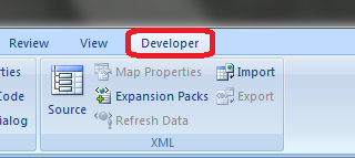
To write VBA, you’ll need to add the Developer tab to the ribbon, so you’ll see the ribbon like this.

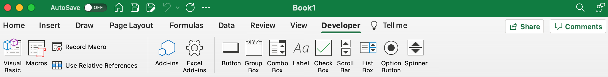
To add the Developer tab to the ribbon:

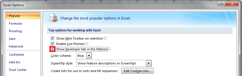
On the File tab, go to Options > Customize Ribbon.
Under Customize the Ribbon and under Main Tabs, select the Developer check box.

After you show the tab, the Developer tab stays visible, unless you clear the check box or have to reinstall Excel. For more information, see Microsoft help documentation.

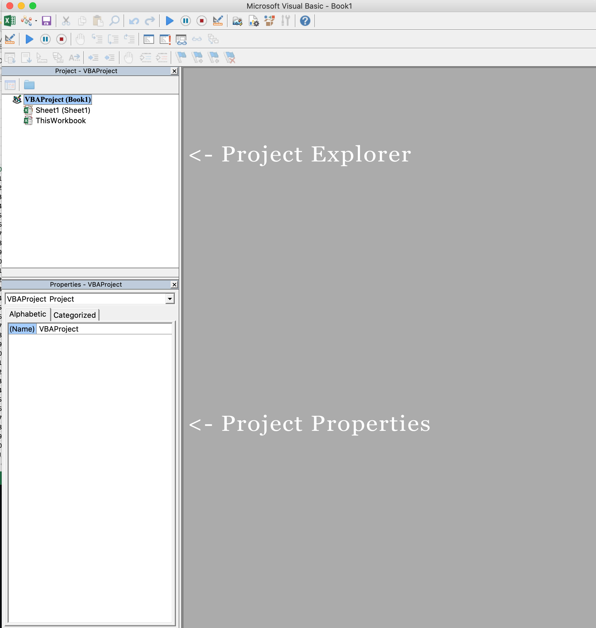
VBA Editor

Navigate to the Developer Tab, and click the Visual Basic button. A new window will pop up — this is the Visual Basic Editor. For the purposes of this tutorial, you just need to be familiar with the Project Explorer pane and the Property Properties pane.

Excel VBA Examples

First, let’s create a file for us to play around in.

Open a new Excel file
Save it as a macro-enabled workbook (. xlsm)
Select the Developer tab
Open the VBA Editor

Let’s rock and roll with some easy examples to get you writing code in a spreadsheet using Visual Basic.

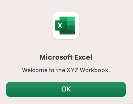
Example #1: Display a Message when Users Open the Excel Workbook

In the VBA Editor, select Insert -> New Module

Write this code in the Module window (don’t paste!):

Sub Auto_Open()
MsgBox («Welcome to the XYZ Workbook.»)
End Sub

Save, close the workbook, and reopen the workbook. This dialog should display.

Ta da!

How is it doing that?

Depending on your familiarity with programming, you may have some guesses. It’s not particularly complex, but there’s quite a lot going on:

Sub (short for “Subroutine): remember from the beginning, “a group of VBA statements that performs one or more actions.”
Auto_Open: this is the specific subroutine. It automatically runs your code when the Excel file opens — this is the event that triggers the procedure. Auto_Open will only run when the workbook is opened manually; it will not run if the workbook is opened via code from another workbook (Workbook_Open will do that, learn more about the difference between the two).
By default, a subroutine’s access is public. This means any other module can use this subroutine. All examples in this tutorial will be public subroutines. If needed, you can declare subroutines as private. This may be needed in some situations. Learn more about subroutine access modifiers.
msgBox: this is a function — a group of VBA statements that performs one or more actions and returns a value. The returned value is the message “Welcome to the XYZ Workbook.”

In short, this is a simple subroutine that contains a function.

When could I use this?

Maybe you have a very important file that is accessed infrequently (say, once a quarter), but automatically updated daily by another VBA procedure. When it is accessed, it’s by many people in multiple departments, all across the company.

Problem: Most of the time when users access the file, they are confused about the purpose of this file (why it exists), how it is updated so often, who maintains it, and how they should interact with it. New hires always have tons of questions, and you have to field these questions over and over and over again.
Solution: create a user message that contains a concise answer to each of these frequently answered questions.

Real World Examples

Use the MsgBox function to display a message when there is any event: user closes an Excel workbook, user prints, a new sheet is added to the workbook, etc.
Use the MsgBox function to display a message when a user needs to fulfill a condition before closing an Excel workbook
Use the InputBox function to get information from the user

Example #2: Allow User to Execute another Procedure

In the VBA Editor, select Insert -> New Module

Write this code in the Module window (don’t paste!):

Sub UserReportQuery()
Dim UserInput As Long
Dim Answer As Integer
UserInput = vbYesNo
Answer = MsgBox(«Process the XYZ Report?», UserInput)
If Answer = vbYes Then ProcessReport
End Sub

Sub ProcessReport()
MsgBox («Thanks for processing the XYZ Report.»)
End Sub

Save and navigate back to the Developer tab of Excel and select the “Button” option. Click on a cell and assign the UserReportQuery macro to the button.

Now click the button. This message should display:

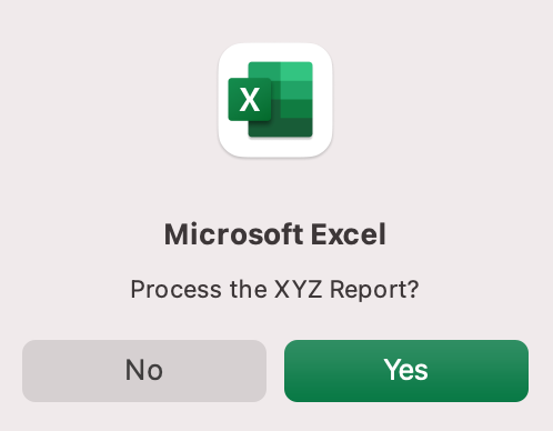
Click “yes” or hit Enter.

Once again, tada!

Please note that the secondary subroutine, ProcessReport, could be anything. I’ll demonstrate more possibilities in example #3. But first…

How is it doing that?

This example builds on the previous example and has quite a few new elements. Let’s go over the new stuff:

Dim UserInput As Long: Dim is short for “dimension” and allows you to declare variable names. In this case, UserInput is the variable name and Long is the data type. In plain English, this line means “Here’s a variable called “UserInput”, and it’s a Long variable type.”
Dim Answer As Integer: declares another variable called “Answer,” with a data type of Integer. Learn more about data types here.
UserInput = vbYesNo: assigns a value to the variable. In this case, vbYesNo, which displays Yes and No buttons. There are many button types, learn more here.
Answer = MsgBox(“Process the XYZ Report?”, UserInput): assigns the value of the variable Answer to be a MsgBox function and the UserInput variable. Yes, a variable within a variable.
If Answer = vbYes Then ProcessReport: this is an “If statement,” a conditional statement, which allows us to say if x is true, then do y. In this case, if the user has selected “Yes,” then execute the ProcessReport subroutine.

When could I use this?

This could be used in many, many ways. The value and versatility of this functionality is more so defined by what the secondary subroutine does.

For example, maybe you have a file that is used to generate 3 different weekly reports. These reports are formatted in dramatically different ways.

Problem: Each time one of these reports needs to be generated, a user opens the file and changes formatting and charts; so on and so forth. This file is being edited extensively at least 3 times per week, and it takes at least 30 minutes each time it’s edited.
Solution: create 1 button per report type, which automatically reformats the necessary components of the reports and generates the necessary charts.

Real World Examples

Create a dialog box for user to automatically populate certain information across multiple sheets
Use the InputBox function to get information from the user, which is then populated across multiple sheets

Example #3: Add Numbers to a Range with a For-Next Loop

For loops are very useful if you need to perform repetitive tasks on a specific range of values — arrays or cell ranges. In plain English, a loop says “for each x, do y.”

In the VBA Editor, select Insert -> New Module

Write this code in the Module window (don’t paste!):

Sub LoopExample()
Dim X As Integer
For X = 1 To 100
Range(«A» & X).Value = X
Next X
End Sub

Save and navigate back to the Developer tab of Excel and select the Macros button. Run the LoopExample macro.

This should happen:

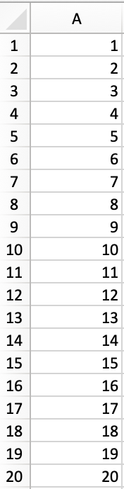
Etc, until the 100th row.

How is it doing that?

Dim X As Integer: declares the variable X as a data type of Integer.
For X = 1 To 100: this is the start of the For loop. Simply put, it tells the loop to keep repeating until X = 100. X is the counter. The loop will keep executing until X = 100, execute one last time, and then stop.
Range(«A» & X).Value = X: this declares the range of the loop and what to put in that range. Since X = 1 initially, the first cell will be A1, at which point the loop will put X into that cell.
Next X: this tells the loop to run again

When could I use this?

The For-Next loop is one of the most powerful functionalities of VBA; there are numerous potential use cases. This is a more complex example that would require multiple layers of logic, but it communicates the world of possibilities in For-Next loops.

Maybe you have a list of all products sold at your bakery in Column A, the type of product in Column B (cakes, donuts, or muffins), the cost of ingredients in Column C, and the market average cost of each product type in another sheet.

You need to figure out what should be the retail price of each product. You’re thinking it should be the cost of ingredients plus 20%, but also 1.2% under market average if possible. A For-Next loop would allow you to do this type of calculation.

Real World Examples

Use a loop with a nested if statement to add specific values to a separate array only if they meet certain conditions
Perform mathematical calculations on each value in a range, e.g. calculate additional charges and add them to the value
Loop through each character in a string and extract all numbers
Randomly select a number of values from an array

Conclusion

Now that we’ve talked about pizza and muffins and oh-yeah, how to write VBA code in Excel spreadsheets, let’s do a learning check. See if you can answer these questions.

What is VBA?
How do I get set up to start using VBA in Excel?
Why and when would you use VBA?
What are some problems I could solve with VBA?

If you have a fair idea of how to you could answer these questions, then this was successful.

Whether you’re an occasional user or a power user, I hope this tutorial provided useful information about what can be accomplished with just a bit of code in your Excel spreadsheets.

Happy coding!

Learning Resources

Excel VBA Programming for Dummies, John Walkenbach
Get Started with VBA, Microsoft Documentation
Learning VBA in Excel, Lynda

A bit about me

I’m Chloe Tucker, an artist and developer in Portland, Oregon. As a former educator, I’m continuously searching for the intersection of learning and teaching, or technology and art. Reach out to me on Twitter @_chloetucker and check out my website at chloe.dev.

Learn to code for free. freeCodeCamp’s open source curriculum has helped more than 40,000 people get jobs as developers. Get started

Источник

Время на прочтение
7 мин

Количество просмотров 312K

Приветствую всех.

В этом посте я расскажу, что такое VBA и как с ним работать в Microsoft Excel 2007/2010 (для более старых версий изменяется лишь интерфейс — код, скорее всего, будет таким же) для автоматизации различной рутины.

VBA (Visual Basic for Applications) — это упрощенная версия Visual Basic, встроенная в множество продуктов линейки Microsoft Office. Она позволяет писать программы прямо в файле конкретного документа. Вам не требуется устанавливать различные IDE — всё, включая отладчик, уже есть в Excel.

Еще при помощи Visual Studio Tools for Office можно писать макросы на C# и также встраивать их. Спасибо, FireStorm.

Сразу скажу — писать на других языках (C++/Delphi/PHP) также возможно, но требуется научится читать, изменять и писать файлы офиса — встраивать в документы не получится. А интерфейсы Microsoft работают через COM. Чтобы вы поняли весь ужас, вот Hello World с использованием COM.

Поэтому, увы, будем учить Visual Basic.

Чуть-чуть подготовки и постановка задачи

Итак, поехали. Открываем Excel.

Для начала давайте добавим в Ribbon панель «Разработчик». В ней находятся кнопки, текстовые поля и пр. элементы для конструирования форм.

Появилась вкладка.

Теперь давайте подумаем, на каком примере мы будем изучать VBA. Недавно мне потребовалось красиво оформить прайс-лист, выглядевший, как таблица. Идём в гугл, набираем «прайс-лист» и качаем любой, который оформлен примерно так (не сочтите за рекламу, пожалуйста):

То есть требуется, чтобы было как минимум две группы, по которым можно объединить товары (в нашем случае это будут Тип и Производитель — в таком порядке). Для того, чтобы предложенный мною алгоритм работал корректно, отсортируйте товары так, чтобы товары из одной группы стояли подряд (сначала по Типу, потом по Производителю).

Результат, которого хотим добиться, выглядит примерно так:

Разумеется, если смотреть прайс только на компьютере, то можно добавить фильтры и будет гораздо удобнее искать нужный товар. Однако мы хотим научится кодить и задача вполне подходящая, не так ли?

Кодим

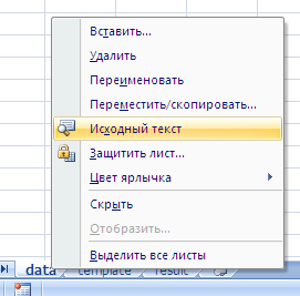
Для начала требуется создать кнопку, при нажатии на которую будет вызываться наша програма. Кнопки находятся в панели «Разработчик» и появляются по кнопке «Вставить». Вам нужен компонент формы «Кнопка». Нажали, поставили на любое место в листе. Далее, если не появилось окно назначения макроса, надо нажать правой кнопкой и выбрать пункт «Назначить макрос». Назовём его FormatPrice. Важно, чтобы перед именем макроса ничего не было — иначе он создастся в отдельном модуле, а не в пространстве имен книги. В этому случае вам будет недоступно быстрое обращение к выделенному листу. Нажимаем кнопку «Новый».

И вот мы в среде разработки VB. Также её можно вызвать из контекстного меню командой «Исходный текст»/«View code».

Перед вами окно с заглушкой процедуры. Можете его развернуть. Код должен выглядеть примерно так:

Sub FormatPrice()End Sub

Напишем Hello World:

Sub FormatPrice() MsgBox "Hello World!" End Sub

И запустим либо щелкнув по кнопке (предварительно сняв с неё выделение), либо клавишей F5 прямо из редактора.

Тут, пожалуй, следует отвлечься на небольшой ликбез по поводу синтаксиса VB. Кто его знает — может смело пропустить этот раздел до конца. Основное отличие Visual Basic от Pascal/C/Java в том, что команды разделяются не ;, а переносом строки или двоеточием (:), если очень хочется написать несколько команд в одну строку. Чтобы понять основные правила синтаксиса, приведу абстрактный код.

Примеры синтаксиса

' Процедура. Ничего не возвращает ' Перегрузка в VBA отсутствует Sub foo(a As String, b As String) ' Exit Sub ' Это значит "выйти из процедуры" MsgBox a + ";" + b End Sub' Функция. Вовращает Integer Function LengthSqr(x As Integer, y As Integer) As Integer ' Exit Function LengthSqr = x * x + y * y End FunctionSub FormatPrice() Dim s1 As String, s2 As String s1 = "str1" s2 = "str2" If s1 <> s2 Then foo "123", "456" ' Скобки при вызове процедур запрещены End IfDim res As sTRING ' Регистр в VB не важен. Впрочем, редактор Вас поправит Dim i As Integer ' Цикл всегда состоит из нескольких строк For i = 1 To 10 res = res + CStr(i) ' Конвертация чего угодно в String If i = 5 Then Exit For Next iDim x As Double x = Val("1.234") ' Парсинг чисел x = x + 10 MsgBox xOn Error Resume Next ' Обработка ошибок - игнорировать все ошибки x = 5 / 0 MsgBox xOn Error GoTo Err ' При ошибке перейти к метке Err x = 5 / 0 MsgBox "OK!" GoTo ne


Err:

    MsgBox 
"Err!"
ne:

On Error GoTo 0 ' Отключаем обработку ошибок ' Циклы бывает, какие захотите Do While True Exit DoLoop 'While True Do 'Until False Exit Do Loop Until False ' А вот при вызове функций, от которых хотим получить значение, скобки нужны. ' Val также умеет возвращать Integer Select Case LengthSqr(Len("abc"), Val("4")) Case 24 MsgBox "0" Case 25 MsgBox "1" Case 26 MsgBox "2" End Select' Двухмерный массив. ' Можно также менять размеры командой ReDim (Preserve) - см. google Dim arr(1 to 10, 5 to 6) As Integer arr(1, 6) = 8Dim coll As New Collection Dim coll2 As Collection coll.Add "item", "key" Set coll2 = coll ' Все присваивания объектов должны производится командой Set MsgBox coll2("key") Set coll2 = New Collection MsgBox coll2.Count End Sub

Грабли-1. При копировании кода из IDE (в английском Excel) есь текст конвертируется в 1252 Latin-1. Поэтому, если хотите сохранить русские комментарии — надо сохранить крокозябры как Latin-1, а потом открыть в 1251.

Грабли-2. Т.к. VB позволяет использовать необъявленные переменные, я всегда в начале кода (перед всеми процедурами) ставлю строчку Option Explicit. Эта директива запрещает интерпретатору заводить переменные самостоятельно.

Грабли-3. Глобальные переменные можно объявлять только до первой функции/процедуры. Локальные — в любом месте процедуры/функции.

Еще немного дополнительных функций, которые могут пригодится: InPos, Mid, Trim, LBound, UBound. Также ответы на все вопросы по поводу работы функций/их параметров можно получить в MSDN.

Надеюсь, что этого Вам хватит, чтобы не пугаться кода и самостоятельно написать какое-нибудь домашнее задание по информатике. По ходу поста я буду ненавязчиво знакомить Вас с новыми конструкциями.

Кодим много и под Excel

В этой части мы уже начнём кодить нечто, что умеет работать с нашими листами в Excel. Для начала создадим отдельный лист с именем result (лист с данными назовём data). Теперь, наверное, нужно этот лист очистить от того, что на нём есть. Также мы «выделим» лист с данными, чтобы каждый раз не писать длинное обращение к массиву с листами.

Sub FormatPrice() Sheets("result").Cells.Clear Sheets("data").Activate End Sub

Работа с диапазонами ячеек

Вся работа в Excel VBA производится с диапазонами ячеек. Они создаются функцией Range и возвращают объект типа Range. У него есть всё необходимое для работы с данными и/или оформлением. Кстати сказать, свойство Cells листа — это тоже Range.

Примеры работы с Range

Sheets("result").Activate Dim r As Range Set r = Range("A1") r.Value = "123" Set r = Range("A3,A5") r.Font.Color = vbRed r.Value = "456" Set r = Range("A6:A7") r.Value = "=A1+A3"

Теперь давайте поймем алгоритм работы нашего кода. Итак, у каждой строчки листа data, начиная со второй, есть некоторые данные, которые нас не интересуют (ID, название и цена) и есть две вложенные группы, к которым она принадлежит (тип и производитель). Более того, эти строки отсортированы. Пока мы забудем про пропуски перед началом новой группы — так будет проще. Я предлагаю такой алгоритм:

Считали группы из очередной строки.
Пробегаемся по всем группам в порядке приоритета (вначале более крупные)
1. Если текущая группа не совпадает, вызываем процедуру AddGroup(i, name), где i — номер группы (от номера текущей до максимума), name — её имя. Несколько вызовов необходимы, чтобы создать не только наш заголовок, но и всё более мелкие.
После отрисовки всех необходимых заголовков делаем еще одну строку и заполняем её данными.

Для упрощения работы рекомендую определить следующие функции-сокращения:

Function GetCol(Col As Integer) As String GetCol = Chr(Asc("A") + Col) End FunctionFunction GetCellS(Sheet As String, Col As Integer, Row As Integer) As Range Set GetCellS = Sheets(Sheet).Range(GetCol(Col) + CStr(Row)) End FunctionFunction GetCell(Col As Integer, Row As Integer) As Range Set GetCell = Range(GetCol(Col) + CStr(Row)) End Function

Далее определим глобальную переменную «текущая строчка»: Dim CurRow As Integer. В начале процедуры её следует сделать равной единице. Еще нам потребуется переменная-«текущая строка в data», массив с именами групп текущей предыдущей строк. Потом можно написать цикл «пока первая ячейка в строке непуста».

Глобальные переменные

Option Explicit ' про эту строчку я уже рассказывал Dim CurRow As Integer Const GroupsCount As Integer = 2 Const DataCount As Integer = 3

FormatPrice

Sub FormatPrice() Dim I As Integer ' строка в data CurRow = 1 Dim Groups(1 To GroupsCount) As String Dim PrGroups(1 To GroupsCount) As String


    Sheets(

"data").Activate I = 2 Do While True If GetCell(0, I).Value = "" Then Exit Do ' ... I = I + 1 Loop End Sub

Теперь надо заполнить массив Groups:

На месте многоточия

Dim I2 As Integer For I2 = 1 To GroupsCount Groups(I2) = GetCell(I2, I) Next I2 ' ... For I2 = 1 To GroupsCount ' VB не умеет копировать массивы PrGroups(I2) = Groups(I2) Next I2 I = I + 1

И создать заголовки:

На месте многоточия в предыдущем куске

For I2 = 1 To GroupsCount If Groups(I2) <> PrGroups(I2) Then Dim I3 As Integer For I3 = I2 To GroupsCount AddHeader I3, Groups(I3) Next I3 Exit For End If Next I2

Не забудем про процедуру AddHeader:

Перед FormatPrice

Sub AddHeader(Ty As Integer, Name As String) GetCellS("result", 1, CurRow).Value = Name CurRow = CurRow + 1 End Sub

Теперь надо перенести всякую информацию в result

For I2 = 0 To DataCount - 1 GetCellS("result", I2, CurRow).Value = GetCell(I2, I) Next I2

Подогнать столбцы по ширине и выбрать лист result для показа результата

После цикла в конце FormatPrice

Sheets("Result").Activate Columns.AutoFit

Всё. Можно любоваться первой версией.

Некрасиво, но похоже. Давайте разбираться с форматированием. Сначала изменим процедуру AddHeader:

Sub AddHeader(Ty As Integer, Name As String) Sheets("result").Range("A" + CStr(CurRow) + ":C" + CStr(CurRow)).Merge ' Чтобы не заводить переменную и не писать каждый раз длинный вызов ' можно воспользоваться блоком With With GetCellS("result", 0, CurRow) .Value = Name .Font.Italic = True .Font.Name = "Cambria" Select Case Ty Case 1 ' Тип .Font.Bold = True .Font.Size = 16 Case 2 ' Производитель .Font.Size = 12 End Select .HorizontalAlignment = xlCenter End With CurRow = CurRow + 1 End Sub

Уже лучше:

Осталось только сделать границы. Тут уже нам требуется работать со всеми объединёнными ячейками, иначе бордюр будет только у одной:

Поэтому чуть-чуть меняем код с добавлением стиля границ:

Sub AddHeader(Ty As Integer, Name As String) With Sheets("result").Range("A" + CStr(CurRow) + ":C" + CStr(CurRow)) .Merge .Value = Name .Font.Italic = True .Font.Name = "Cambria" .HorizontalAlignment = xlCenterSelect Case Ty Case 1 ' Тип .Font.Bold = True .Font.Size = 16 .Borders(xlTop).Weight = xlThick Case 2 ' Производитель .Font.Size = 12 .Borders(xlTop).Weight = xlMedium End Select .Borders(xlBottom).Weight = xlMedium ' По убыванию: xlThick, xlMedium, xlThin, xlHairline End With CurRow = CurRow + 1 End Sub

Осталось лишь добится пропусков перед началом новой группы. Это легко:

В начале FormatPrice

Dim I As Integer ' строка в data CurRow = 0 ' чтобы не было пропуска в самом начале Dim Groups(1 To GroupsCount) As String

В цикле расстановки заголовков

If Groups(I2) <> PrGroups(I2) Then CurRow = CurRow + 1 Dim I3 As Integer

В точности то, что и хотели.

Надеюсь, что эта статья помогла вам немного освоится с программированием для Excel на VBA. Домашнее задание — добавить заголовки «ID, Название, Цена» в результат. Подсказка: ~~CurRow = 0~~ CurRow = 1.

Файл можно скачать тут (min.us) или тут (Dropbox). Не забудьте разрешить исполнение макросов. ~~Если кто-нибудь подскажет человеческих файлохостинг, залью туда.~~

Спасибо за внимание.

Буду рад конструктивной критике в комментариях.

UPD: Перезалил пример на Dropbox и min.us.

UPD2: На самом деле, при вызове процедуры с одним параметром скобки можно поставить. Либо использовать конструкцию Call Foo(«bar», 1, 2, 3) — тут скобки нужны постоянно.

Источник

Применение оператора With для упрощения кода VBA Excel и ускорения его работы. Синтаксис оператора With, параметры, поясняющие примеры.

Оператор With предназначен для выполнения последовательности операторов (строк кода) для отдельного объекта или пользовательского типа данных.

Применение оператора With упрощает написание и восприятие кода VBA Excel, а также ускоряет его работу.

Синтаксис

Синтаксис оператора With в VBA Excel:

With object

[statements]

End With

Параметры

Параметры оператора With:

Параметр	Описание
object	Имя объекта или пользовательского типа данных.
statements	Один или несколько операторов (строк кода), которые выполняются в отношении указанного объекта.

Примеры

В следующей процедуре выполняется несколько идущих подряд операторов (строк кода) в отношении одного и того же объекта Range("A1:E5"):

Sub Primer1()

Range(«A1:E5»).Value = «Тест»

Range(«A1:E5»).Interior.Color = vbMagenta

Range(«A1:E5»).Font.Size = 14

Range(«A1:E5»).Font.Color = vbYellow

Range(«A1:E5»).Font.Italic = True

Range(«A1:E5»).Borders.LineStyle = True

End Sub

Если в процедуре выполняется несколько идущих подряд операторов в отношении одного и того же объекта, то оператор With позволяет указать объект только один раз:

Sub Primer2()

With Range(«A1:E5»)

.Value = «Тест»

.Interior.Color = vbMagenta

.Font.Size = 14

.Font.Color = vbYellow

.Font.Italic = True

.Borders.LineStyle = True

End With

End Sub

Такое написание кода делает его более понятным, а выполнение – более быстрым.

Конструкции с оператором With можно вкладывать одну в другую:

Sub Primer3()

With Range(«A1:E5»)

.Value = «Тест»

.Interior.Color = vbMagenta

With .Font

.Size = 14

.Color = vbYellow

.Italic = True

End With

.Borders.LineStyle = True

End With

End Sub

Такой код удобен, когда необходимо выполнить ряд операторов по отношению к некоторому объекту [Range("A1:E5")], а также по отношению к одному из содержащихся в нем объектов [Range("A1:E5").Font].

Примечания

Примечания от разработчика:

После входа в блок With параметр object изменить нельзя. Следовательно, один оператор With не может быть использован для изменения нескольких объектов.
Во вложенном блоке With необходимо указывать полные ссылки на любые элементы объекта из внешнего блока With.
Не рекомендуется использовать переходы в блоки With или из них.

Источник

Excel VBA Code Programming

VBA code can be defined as the code that inputs in the visual basic window to perform a set of instructions or actions in excel and provide results. With the help of VBA code, we can reduce the time to perform a repetitive task, there will not be required much human intervention except to run the program. Now we will see how to open a visual basic window, how to write code in it, how to run, and how to save it.

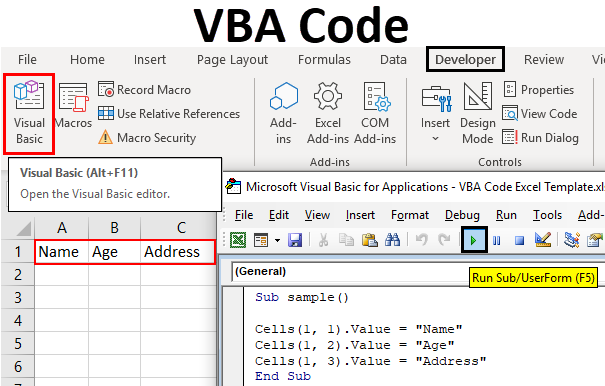
How to Open a Visual Basic Window?

If you want to write the visual basic code, we should write it in a visual basic window. The question here is, where is the visual basic window in excel and how to open it. The answer is to select the Developer menu and under the developer menu, choose Visual Basic as shown in the below image.

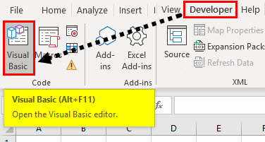
Which will open the blank window as shown below.

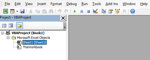
Easy and looks cool right. But incase if excel does not have Developer tab. We need to add the developer tab with the below steps.

Step 1: Click on File Option.

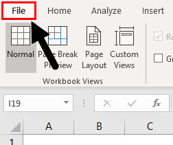
Step 2: Drop-down appears, click on Options tab.

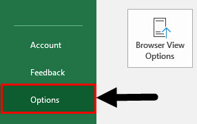
Step 3: Once you click on “Options”, a dialog box appears as shown below and click on the Customize Ribbon option.

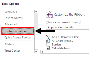
Step 4: When we drag down in the customize ribbon options we will find an option for Developer (Custom) we need to check that box which will enable us to use VBA in excel.

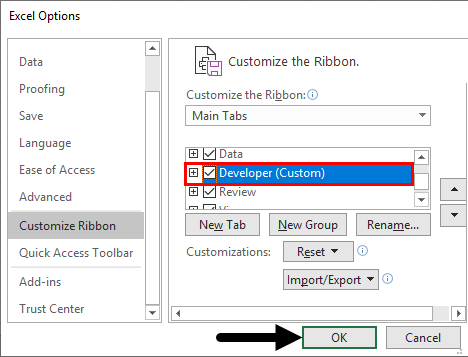
Another easy way to open the Visual basic window is by pressing Alt+F11

Where to Write Code in Excel VBA?

By default, there will be two modules available to write your code, one is sheet1 module and workbook module.

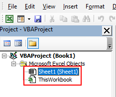
If we add multiple sheets in our workbook it will allow different sheet modules here.

Sheet Module Code: Whatever the event code we write in the sheet module it will apply for that sheet alone.

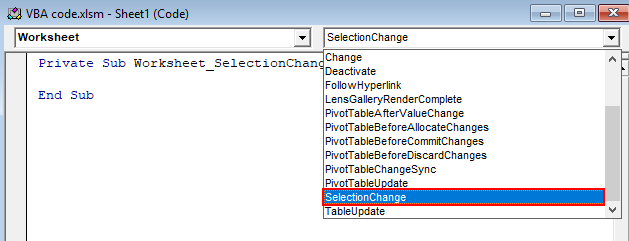
You may be in confusion what is an event code. VBA comes with multiple events shown in the above screenshot, events like change, deactivate and many more. Whenever that event happened the macro will run.

ThisWorkbook Module

Whatever the code written in this module will apply for all the sheets in the workbook. Suppose if we write an event code for the workbook then whenever that event happened in any of the sheets of the workbook the macro will run. Suppose if we write an event for “New sheet” then whenever we created a new sheet the macro will run for that workbook.

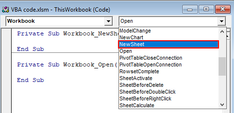
Module: Normally we will write code in modules in VBA. We need to insert the module by clicking on the Insert menu and select the module option to insert a module.

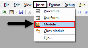
Similarly, we can insert a class module and user form also. These are the modules where we can write our code. Depend on the type of requirement we should choose the module and write the code in it.

Examples to Write and Run Code in Excel VBA

Below are the different examples to write and run the code using VBA Code in Excel.

You can download this VBA Code Excel Template here – VBA Code Excel Template

Example #1 – Macro Code using a Normal Module

Now we will see a sample macro code using a normal module. When we insert a new module, the empty window will look like below.

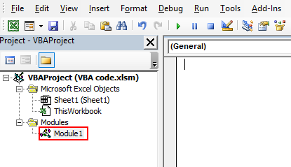
Follow the below steps to write code in excel VBA.

Step 1: Any program in VBA starts with sub keyword and program name with open and close brackets as below. When we enter after the brackets automatically “End Sub” will appear.

Code:

Sub sample()

End Sub

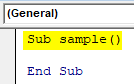
Step 2: In between, we should write our code.

Code:

Sub sample()

Cells(1, 1).Value = "Name"
Cells(1, 2).Value = "Age"
Cells(1, 3).Value = "Address"

End Sub

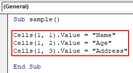
In the above macro, I wrote a sample code like when I run the macro first three cells should fill with Name, Age and Address. Cells(1,1).value represents the cell of row1 and column1 value.

Step 3: We can run the code by pressing F5 or click on the run button at the top which is marked in Black colored box.

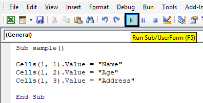
Step 4: Once we click on run, a pop up will ask for a run as below. If multiple macros are available need to choose the correct macro and click on the run button.

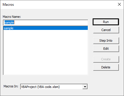
Step 5: Go to excel and check whether the results are appearing or not as below.

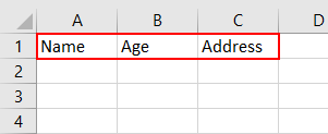
Example #2 – Attaching a Macro to a Shape

If we want to run the macro from the worksheet itself with the help of a shape, we can do that. Follow the below steps to assign the macro to shapes.

Step 1: Go to Insert, and Select the shape as per your wish.

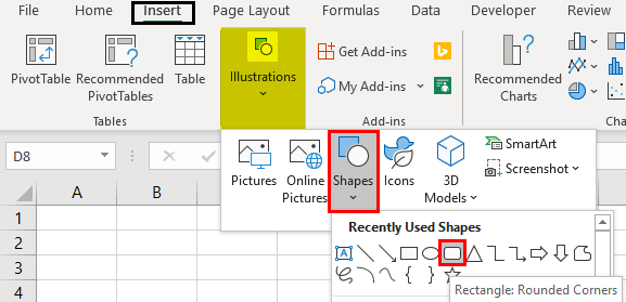
Step 2: After selecting the shape, draw this on your worksheet.

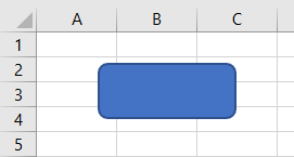
Step 3: Now, we can write a text like “click here” or “run Macro” in that shape. For adding the text just right click on a shape and select Edit Text

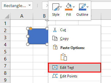
Step 4: Add the word as per your wish. I have added the word as “Run Macro”.

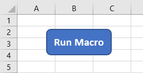
Step 5: Now, we need to assign the macro to that shape, for that select the shape and right click and choose “Assign Macro” option.

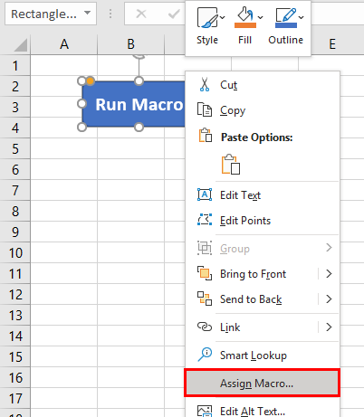
Step 6: A pop-up box will come asking for macro selection. Select the macro name and click on the Ok button.

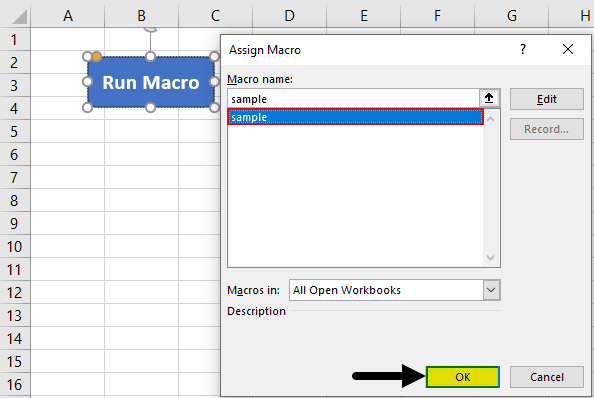
Step 7: Now, if we click on the shape the macro will run and give the result as below.

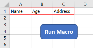
How to Save the Macro Workbook?

We all know how to save a workbook. Saving macro workbook is also same but one small change will be there. We have two different ways to save our macro files.

Macro enabled workbook
Macro enabled template

When you are saving the workbook, we need to choose the file type from the list of file type options as below.

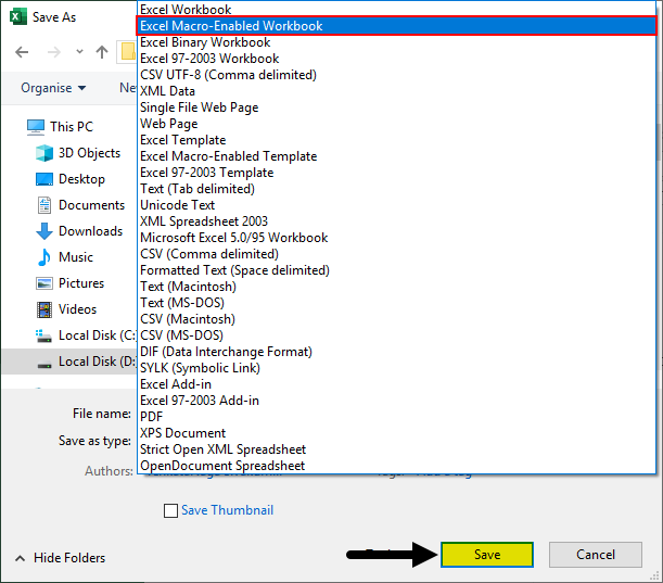
By default, we can use the “Excel macro-enabled workbook”. In case if you want to use as standard file as a starting point for other files then use “Excel macro-enabled template” format.

Things to Remember

Add the developer tab in case if it is not available in the menu ribbon.
If want to create a simple basic macro, try to use recording a macro as it does not need any coding not even need to go to the visual basic screen. Click on record macro option from the developer tab and give macro name to perform the required steps. It will record the steps you are performing, once it is over, stops recording and can run the macro now as to how we run the macro in the above steps.
Choose the module type depending on the requirement, by default we can write in a normal module.
Do not forget to save the file in the macro-enabled format then only the workbook will be a macro-enabled workbook.

Excel VBA Code

VBA, also known as Visual Basic Applications, is a programming language for Excel. Not only Excel but for most Microsoft Office programs. We can write a set of instructions in a Visual Basic Editor that performs certain tasks for us, known as code in VBA.

In Excel, we can find VBA under the “Developer” tab for developers. To access the “Developer” tab, we need to enable it first, and then we can access it from the tab or by the keyboard shortcut ALT + F11. A combination of codes makes a procedure, which is also known as macros in VBA. So, in other words, macros are a set of codes, a programming language written together.

If you are new to VBA and have no idea about it, this article is for you.

Excel VBA Code
- Enable Developer Tab
- Examples to Use Excel VBA Code
  - #1 – Paste Code in Module
  - #2 – Save the Workbook with VBA Code
  - #3 – Assign Macro Code to Shapes
- Recommended Articles

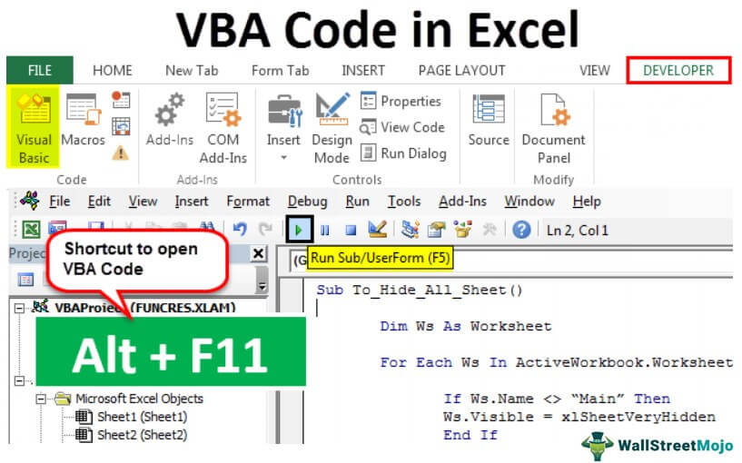
You are free to use this image on your website, templates, etc, Please provide us with an attribution linkArticle Link to be Hyperlinked
For eg:
Source: VBA Code (wallstreetmojo.com)

Enable Developer Tab

First, you must ensure that the developer tab in excelEnabling the developer tab in excel can help the user perform various functions for VBA, Macros and Add-ins like importing and exporting XML, designing forms, etc. This tab is disabled by default on excel; thus, the user needs to enable it first from the options menu.read more is on the ribbon.

If your Excel is not showing the “Developer” tab, follow the steps below to enable the “Developer” tab in your Excel.

Next, go to “File.”
Click on “Options.”
Go to “Customize Ribbon” in excel.
Check the “Developer” tab on the right side. Once you select the options, click on “OK.”

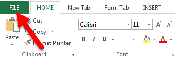
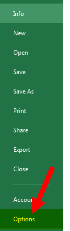
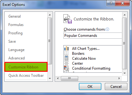
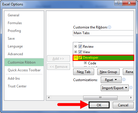
Examples to Use Excel VBA Code

#1 – Paste Code in Module

To write VBA code, you first need to go to the “Developer” tab and click on “Visual Basic.”

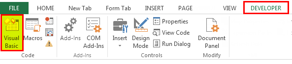
You can press the excel shortcut keyAn Excel shortcut is a technique of performing a manual task in a quicker way.read more “ALT + F11” to open Visual Basic.

As you open the visual basic, you will see a window like the one below.

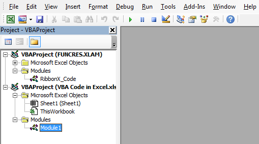
Next, go to “Insert” and click on “Module.”

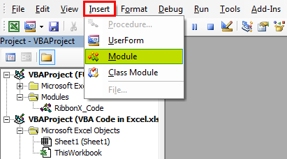
As soon as you click on the “Module,” it will insert it, and you can see the “Module” name. And also, you will see a white plain board on the right.

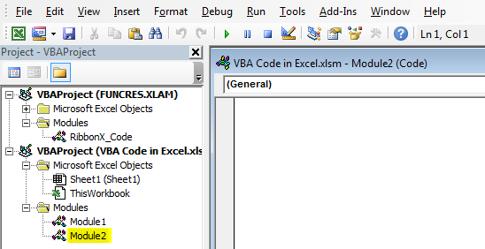
On the white plain board, you need to paste your copied code.

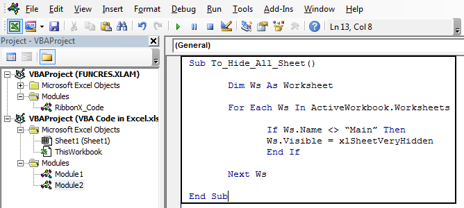
After pasting the code, you need to execute it.

We can conduct the execution process by pressing the shortcut key F5 or clicking the green run button on the top.

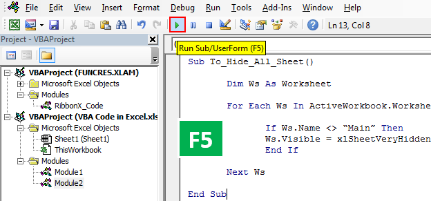
It will execute the copied VBA code in your window.

#2 – Save the Workbook with VBA Code

We know you do not need any special introduction to save the Excel file. But when it comes to the VBA code in the Excel workbook, you need one special introduction.

If you have already saved the workbook and just copied the VBA code, you need to change the file extension because when you click on the “Save” option, you will see the alert message below.

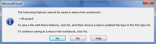
It says the workbook you are trying to save contains a VB project, and it cannot save as a normal Excel workbook. So instead, save this workbook as a “Macro-Enabled” workbook.

Click on “Save As” or press the F12 key. You will see below a window.

Save as

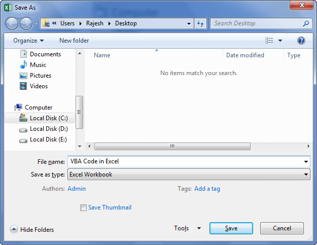
Enter the file name as per your wish but select the “Save as type” as “Excel Macro-Enabled Workbook (*.xlsm).

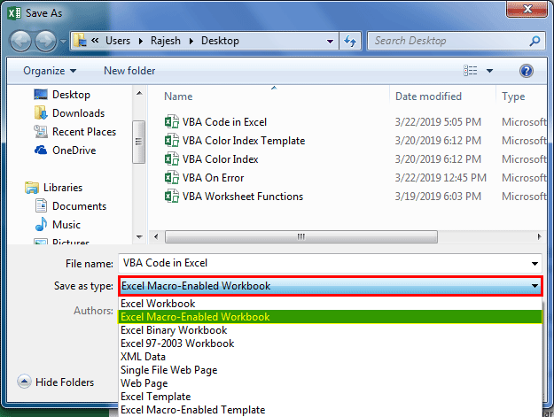
Click “OK” to save the workbook as “Macro-Enabled Workbook.”

Save

#3 – Assign Macro Code to Shapes

Whenever we need to run VBA, we need to return to the visual basic editor and run. It is a time-consuming process.

We can assign a macro by its name to one of the shapes. Follow the below steps to assign the excel macroA macro in excel is a series of instructions in the form of code that helps automate manual tasks, thereby saving time. Excel executes those instructions in a step-by-step manner on the given data. For example, it can be used to automate repetitive tasks such as summation, cell formatting, information copying, etc. thereby rapidly replacing repetitious operations with a few clicks.
read more to shapes.

Step 1: Go to “Insert” and select the shape per your wish.

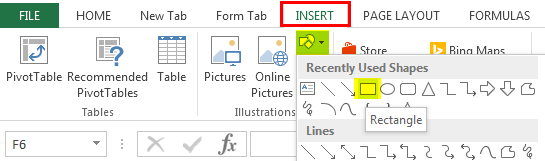
Step 2: After selecting the shape, draw this on your worksheet, ideally, away from the data.

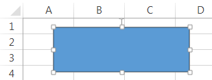
Step 3: Right-click and select “Edit Text.”

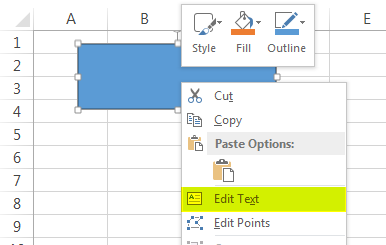
Step 4: Add the word as per your wish. We have added the word “Click Here to Run the Macro.”

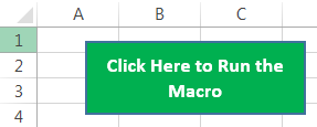
Step 5: Again, right-click and select the option to assign a macro.

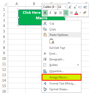
Step 6: Now, we will see all the macro lists. Select the macro name you wish to assign.

Step 7: Click on “OK.” Now, this button holds the macro code. Whenever you click on this button, it will execute this code.

PART ONE: How to use VBA Macros

What is VBA?

Visual Basic for Applications (VBA) is the programming language created by Microsoft to control parts of their applications. Most things which you can do with the mouse or keyboard in the Microsoft Office suite, you can also do using VBA. For example, in Excel, you can create a chart; you can also create a chart using VBA, it is just another method of achieving the same thing.

Advantages of using VBA

Since VBA code can do the same things as we could with the mouse or keyboard, why bother to use VBA at all?

Saves time:

VBA code will operate at the speed your computer will allow, which is still significantly faster than you can operate. For example, if you have to open 10 workbooks, print the documents, then close the workbook, it might take you 2 minutes with a mouse and keyboard, but with VBA it could take seconds.

Reduces errors:

Do you ever click the wrong icons or type the wrong words? Me too, but VBA doesn’t. It will do the same task over and over again, without making any errors. Don’t get me wrong, you still have to program the VBA code correctly. If you tell it to do the wrong things 10 times, then it will. But if we can get it right, then it can remove the errors created by human interaction.

Completes repetitive actions without complaining:

Have you ever had to carry out the same action many times? Maybe creating 100 charts, or printing 100 documents, or changing the heading on 100 spreadsheets. That’s not fun, nobody wants to do that. But VBA is more than happy to do it for you. It can do the same thing in a repetitive way (without complaining). In fact, repetitive tasks is one of the things VBA does best.

Integration with other applications:

You can use VBA in Word, Access, Excel, Outlook and many other programs, including Windows itself. But it doesn’t end there, you can use VBA in Excel to control Word and PowerPoint, without even needing to open those applications.

What is programming?

Programming is simply writing words in a way which a computer can understand. However, computers are not particularly flexible, so we have to be very specific about what we want the computer to do, and how we tell it to do it. The skill of programming is learning how to convey the request to the computer as clearly, as simply and as efficiently as possible.

What is the difference between a Macro and VBA?

This is a common question which can be confusing. Put simply, VBA is the language used to write a macro – just in the same way as a paragraph might be written using the English language.

The terms ‘macro’ and ‘VBA’ are often used interchangeably.

The golden rule of learning VBA

If you are still learning to write VBA, there is one thing which will help you. While it may be common practice, to copy and paste code, it will not help you to learn VBA quickly. Here is the one rule I am going to ask you to stick to… type out the code yourself.

Why am I asking you to do this? Because it will help you learn the VBA language much faster.

Let’s get started

Now you know what VBA is, why you should use it, and the golden rule, so there is only one thing left to do… let’s get started!

Setting up Excel

Before you can get stuck in with using the code in this post, you must first have Excel set up correctly. This involves:

Ensuring the correct macro security settings have been applied
Enabling the Developer ribbon.

Macro security settings

Macros can be used for malicious purposes, such as installing a virus, recording key-strokes, etc. This can be blocked with the security settings. However, if the settings are set too high, you cannot run any macros, or too low, you will not be protected. Neither of these is a good option.

Let’s apply suitable settings which will give you the power to decide when to allow macros or not.

In Excel, click File > Options
In the Excel Options dialog box, click Trust Centre > Trust Centre Settings…
In the Trust Centre dialog box, click Macro Settings > Disable all macros with notification.
Click OK to close the Trust Centre, then OK again to close the Excel Options.

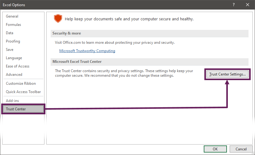
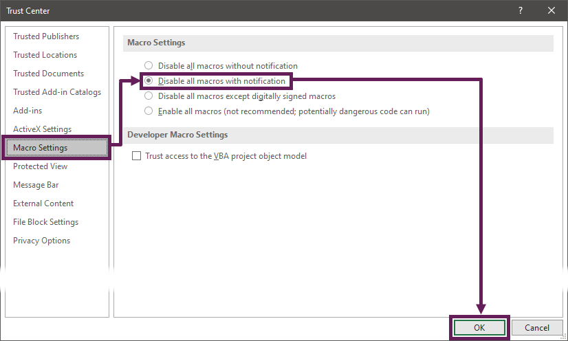
Workbooks containing macros will now be automatically disabled until you click the Enable Content button at the top of the screen.

Enable the Developer ribbon

The Developer ribbon is the place where all the VBA tools are kept. It is unlikely that this is already enabled, unless you or your IT department have already done so.

Look at the top of your Excel Window if you see the word ‘Developer’ in the menu options, then you are ready to go. You can skip straight ahead to the next part. However, if the ‘Developer’ ribbon is not there, just follow these instructions.

In Excel, click File > Options
In the Excel Options dialog box, click Customize Ribbon
Ensure the Developer option is checked
Click OK to close the Excel Options

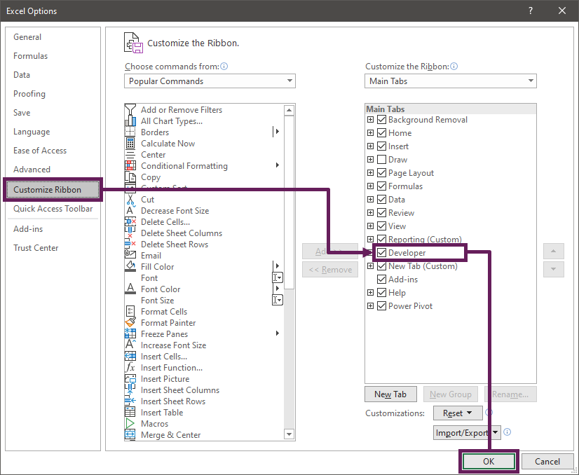
The Developer ribbon should now be visible at the top of the Excel window.

File format for macro enabled files

To save a workbook containing a macro, the standard .xlsx format will not work.

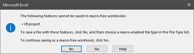
Generally, the .xlsm (Excel Macro-Enabled Workbook) file format should be used for workbooks containing macros. However .xlam (Excel Add-in), .xlsb (Excel Binary Workbook) and .xltx (Excel Macro-Enabled Template) are scenario specific formats which can also contain macros.

The legacy .xls and .xla file formats can both contain macros. They were superseded in 2007, and should now be avoided.

The basic rule is… if you don’t know, go for .xlsm.

Personal macro workbook

If we want macros to be reusable for many workbooks, often the best place to save them is in the personal macro workbook.

A personal macro workbook is a hidden file which opens whenever the Excel application opens.

How to create a personal macro workbook?

A personal macro workbook does not exist by default; we have to create it. There are many ways to do this, but the easiest is to let Excel do it for us.

In the ribbon, click Developer > Record Macro.
In the Record Macro dialog box, select Personal Macro Workbook from the drop-down list.
Click OK.
Do anything in Excel, such as typing your name into cell A1.
Click Developer > Stop Recording
Close all the open workbooks in Excel, this will force the personal macro workbook to be saved. A warning message will appear, click Save.

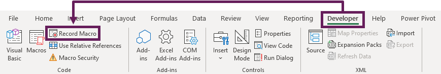
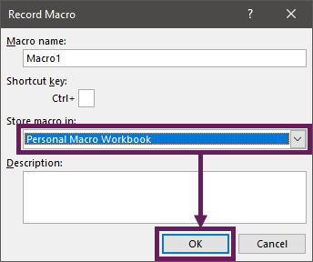
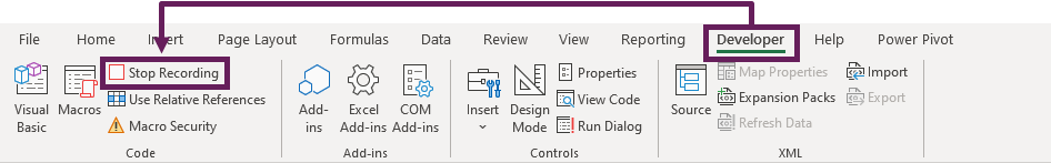
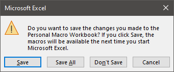
In the next part, we will learn how to use the Visual Basic Editor, which gives us access to the personal macro workbook.

Using the Visual Basic Editor

The Visual Basic Editor (or VBE as it can be known) is the place where we enter or edit VBA code. The Visual Basic Editor is found within the Developer Ribbon

In Excel, click Developer > Visual Basic to open the VBE.

Alternatively, you could use the keyboard; press ALT+F11 (the + indicates that you should hold down the ALT key, press F11, then release the ALT key), which toggles between the Excel window and the VBE.

The Visual Basic Editor Window

The Visual Basic Editor contains four main sections.

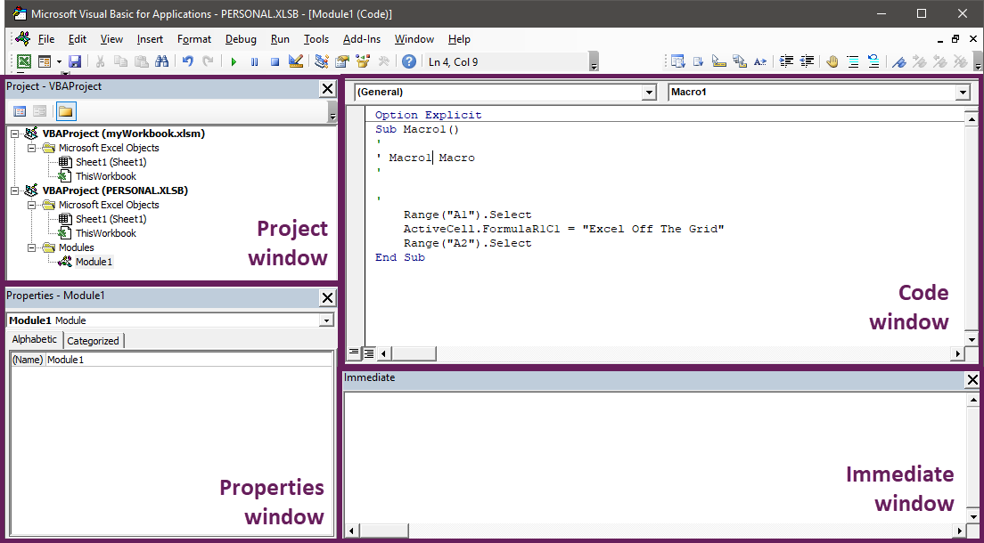
Within the top left of the VBE, we will see a list of items which can contain VBA code (known as the project window)

Double-clicking any sheet name, workbook or module, will open the code window associated with that item. VBA code is entered into the code window.

Unless you have specific reasons, the best option is to enter the macro into a module. To create a module, click Insert > Module within the VBE.

Running a macro

There are many ways to run VBA code. This section is not exhaustive, but is intended to provide an overview of the most common methods.

Running a macro from within Visual Basic Editor

When testing VBA code, it is common to execute that code from the VBE.

Click anywhere within the code, between the Sub and End Sub lines, choose one of the following options:

Click Run > Run Sub/UserForm from the menu at the top of the VBE
Using the keyboard, you can press ALT+F5
Click the play button at the top of the VBE

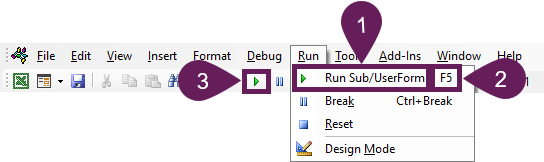
The code you entered will be executed.

Running a macro from within Excel

Once the code has been tested and in working order, it is common to execute it directly within Excel. There are lots of options for this too (including events, or user defined functions), however the three most common methods I will show you are:

Run from the Macro window

Click View > Macros or Developer > Macros
Select the macro from the list and click Run.

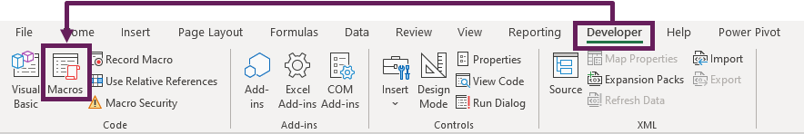
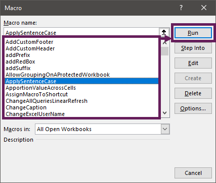
Create a custom ribbon

Having macros always available in the ribbon is a great time saver. Therefore, learning how to customize the ribbon is useful.

In Excel, click File > Options
In the Excel Options dialog box, click Customize Ribbon
Click New Tab to create a new ribbon tab, then click New Group to create a section within the new tab.
In the Choose commands from drop-down, select Macros. Select your macro and click
Add >> to move the macro it into your new group.
Use the Rename… button to give the tab, group or macro a more useful name.
Click OK to close the window.
The new ribbon menu will appear containing your macro. Click the button to run the macro.

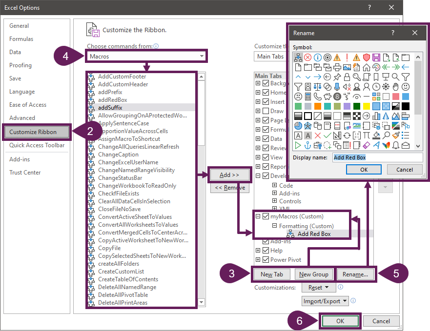
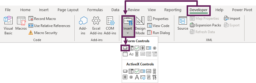
Create a button/shape on a worksheet

Macros can be executed using buttons or shapes on the worksheet.

To create a button, click Developer > Insert > Form Control > Button
Draw a shape on the worksheet to show the location and size of the button
The Assign Macro dialog will appear, select the macro and click OK.
The button will appear. Clicking the button will run the macro
Right-click on the button to change the description

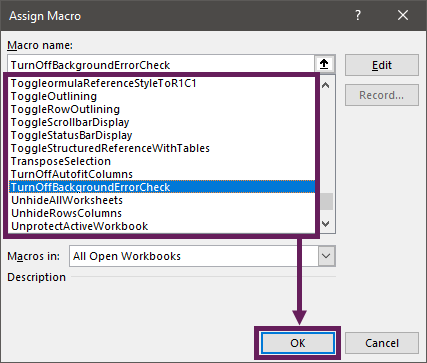
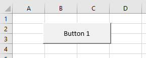
To assign a different macro, right-click on the button and select Assign Macro… from the menu.

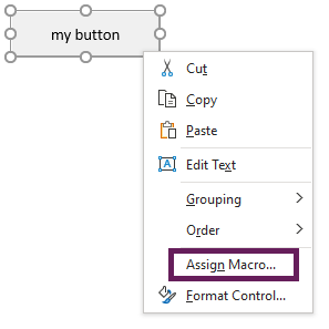
Alternatively, a macro can be assigned to a shape. After creating a shape, right-click on it and select Assign Macro… from the menu, then follow the same process as for a button.

Hide all selected sheets

What does it do?

Hides all the selected sheets.

VBA code

Sub HideAllSelectedSheets()

'Create variable to hold worksheets
Dim ws As Worksheet

'Ignore error if trying to hide the last worksheet
On Error Resume Next

'Loop through each worksheet in the active workbook
For Each ws In ActiveWindow.SelectedSheets

    'Hide each sheet
    ws.Visible = xlSheetHidden

Next ws

'Allow errors to appear
On Error GoTo 0

End Sub

Notes:

Excel requires at least one active worksheet. If all the visible sheets are selected, to avoid an error, the VBA code will not hide the last sheet.

For other examples of hiding worksheets check out these posts:

Macro to hide all sheets except one
Hide all sheets except one with Office Scripts

Unhide all sheets

What does it do?

Makes all worksheets visible.

VBA code

Sub UnhideAllWorksheets()

'Create variable to hold worksheets
Dim ws As Worksheet

'Loop through each worksheet in the active workbook
For Each ws In ActiveWorkbook.Worksheets

    'Unhide each sheet
    ws.Visible = xlSheetVisible

Next ws

End Sub

Protect all selected worksheets

What does it do?

Protects all the selected worksheets with a password determined by the user.

VBA code

Sub ProtectSelectedWorksheets()

Dim ws As Worksheet
Dim sheetArray As Variant
Dim myPassword As Variant

'Set the password
myPassword = Application.InputBox(prompt:="Enter password", _
    Title:="Password", Type:=2)

'The User clicked Cancel
If myPassword = False Then Exit Sub

'Capture the selected sheets
Set sheetArray = ActiveWindow.SelectedSheets

'Loop through each worksheet in the active workbook
For Each ws In sheetArray

    On Error Resume Next

    'Select the worksheet
    ws.Select

    'Protect each worksheet
    ws.Protect Password:=myPassword

    On Error GoTo 0

Next ws

sheetArray.Select

End Sub

Unprotect all worksheets

What does it do?

Unprotects all worksheets with a password determined by the user.

VBA code

Sub UnprotectAllWorksheets()

'Create a variable to hold worksheets
Dim ws As Worksheet

'Create a variable to hold the password
Dim myPassword As Variant

'Set the password
myPassword = Application.InputBox(prompt:="Enter password", _
    Title:="Password", Type:=2)

'The User clicked Cancel
If myPassword = False Then Exit Sub

'Loop through each worksheet in the active workbook
For Each ws In ActiveWindow.SelectedSheets

    'Protect each worksheet
    ws.Unprotect Password:=myPassword

Next ws

End Sub

Lock cells containing formulas

What does it do?

Password protects a single worksheet with cells containing formulas locked, all other cells are unlocked.

VBA code

Sub LockOnlyCellsWithFormulas()

'Create a variable to hold the password
Dim myPassword As Variant

'If more than one worksheet selected exit the macro
If ActiveWindow.SelectedSheets.Count > 1 Then

    'Display error message and exit macro
    MsgBox "Select one worksheet and try again"
    Exit Sub

End If

'Set the password
myPassword = Application.InputBox(prompt:="Enter password", _
    Title:="Password", Type:=2)

'The User clicked Cancel
If myPassword = False Then Exit Sub

'All the following to apply to active sheet
With ActiveSheet

    'Ignore errors caused by incorrect passwords
    On Error Resume Next

    'Unprotect the active sheet
    .Unprotect Password:=myPassword

    'If error occured then exit macro
    If Err.Number <> 0 Then

        'Display message then exit
        MsgBox "Incorrect password"
        Exit Sub

    End If

    'Turn error checking back on
    On Error GoTo 0

    'Remove lock setting from all cells
    .Cells.Locked = False

    'Add lock setting to all cells
    .Cells.SpecialCells(xlCellTypeFormulas).Locked = True

    'Protect the active sheet
    .Protect Password:=myPassword

    End With

End Sub

Hide formulas when protected

What does it do?

When the active sheet is protected, formulas will not be visible in the formula bar. Uses a predefined password of mypassword.

VBA code

Sub HideFormulasWhenProtected()

'Create a variable to hold the password
Dim myPassword As String

'Set the password
myPassword = "myPassword"

'All the following to apply to active sheet
With ActiveSheet

    'Unprotect the active sheet
    .Unprotect Password:=myPassword

    'Hide formulas in all cells
    .Cells.FormulaHidden = True

    'Protect the active sheet
    .Protect Password:=myPassword

End With

End Sub

Save time stamped backup file

What does it do?

Save a backup copy of the workbook with a time stamp.

VBA code

Sub SaveTimeStampedBackup()

'Create variable to hold the new file path
Dim saveAsName As String

'Set the file path
saveAsName = ActiveWorkbook.Path & "" & _
Format(Now, "yymmdd-hhmmss") & " " & ActiveWorkbook.Name

'Save the workbook
ActiveWorkbook.SaveCopyAs Filename:=saveAsName

End Sub

Prepare workbook for saving

What does it do?

The macro will, for each worksheet:

Close all group outlining
Set the view to the normal view
Remove gridlines
Hide all row numbers and column numbers
Select cell A1

The first sheet is selected.

After running the macro, every worksheet in the workbook will be in a tidy state for the next use.

VBA code

Sub PrepareWorkbookForSaving()

'Declare the worksheet variable
Dim ws As Worksheet

'Loop through each worksheet in the active workbook
For Each ws In ActiveWorkbook.Worksheets

    'Activate each sheet
    ws.Activate

    'Close all of groups
    ws.Outline.ShowLevels RowLevels:=1, ColumnLevels:=1

    'Set the view settings to normal
    ActiveWindow.View = xlNormalView

    'Remove the gridlines
    ActiveWindow.DisplayGridlines = False

    'Remove the headings on each of the worksheets
    ActiveWindow.DisplayHeadings = False

    'Get worksheet to display top left
    ws.Cells(1, 1).Select
Next ws

'Find the first visible worksheet and select it
For Each ws In Worksheets

    If ws.Visible = xlSheetVisible Then

        'Select the first visible worksheet
        ws.Select

        'Once the first visible worksheet is found exit the sub
        Exit For

    End If

Next ws

End Sub

Convert merged cells to center across

What does it do?

Changes all single row merged cells into center across formatting.

VBA code

Sub ConvertMergedCellsToCenterAcross()

Dim c As Range
Dim mergedRange As Range

'Loop through all cells in Used range
For Each c In ActiveSheet.UsedRange

    'If merged and single row
    If c.MergeCells = True And c.MergeArea.Rows.Count = 1 Then

        'Set variable for the merged range
        Set mergedRange = c.MergeArea

        'Unmerge the cell and apply Centre Across Selection
        mergedRange.UnMerge
        mergedRange.HorizontalAlignment = xlCenterAcrossSelection

    End If

Next

End Sub

Fit selection to screen

What does it do?

Zoom the screen on the selected cells.

VBA code

Sub FitSelectionToScreen()

'To zoom to a specific area, then select the cells
Range("A1:I15").Select

'Zoom to selection
ActiveWindow.Zoom = True

'Select first cell on worksheet
Range("A1").Select

End Sub

Flip number signage on selected cells

What does it do?

Flips the number signage of all numeric values in the selected cells

VBA code

Sub FlipNumberSignage()

'Create variable to hold cells in the worksheet
Dim c As Range

'Loop through each cell in selection
For Each c In Selection

    'Test if the cell contents is a number
    If IsNumeric(c) Then

        'Convert signage for each cell
        c.Value = -c.Value

    End If

Next c

End Sub

Clear all data cells

What does it do?

Clears all cells in the selection which are constants (i.e. not formulas).

VBA code

Sub ClearAllDataCellsInSelection()

'Clear all hardcoded values in the selected range
Selection.SpecialCells(xlCellTypeConstants).ClearContents

End Sub

Add prefix to each cell in selection

What does it do?

Adds a prefix to each cell in the selected cells (excludes formulas and blanks).

VBA code

Sub AddPrefix()

Dim c As Range
Dim prefixValue As Variant

'Display inputbox to collect prefix text
prefixValue = Application.InputBox(Prompt:="Enter prefix:", _
    Title:="Prefix", Type:=2)

'The User clicked Cancel
If prefixValue = False Then Exit Sub

For Each c In Selection

    'Add prefix where cell is not a formula or blank
    If Not c.HasFormula And c.Value <> "" Then

        c.Value = prefixValue & c.Value

    End If

Next

End Sub

Add suffix to each cell in selection

What does it do?

Adds a suffix to each value in the selected cells (excludes formulas and blanks).

VBA code

Sub AddSuffix()

Dim c As Range
Dim suffixValue As Variant

'Display inputbox to collect prefix text
suffixValue = Application.InputBox(Prompt:="Enter Suffix:", _
    Title:="Suffix", Type:=2)

'The User clicked Cancel
If suffixValue = False Then Exit Sub

    'Loop through each cellin selection
    For Each c In Selection

        'Add Suffix where cell is not a formula or blank
        If Not c.HasFormula And c.Value <> "" Then

            c.Value = c.Value & suffixValue

        End If

Next

End Sub

Reverse row order

What does it do?

Reverses the order of all rows of data in the selection.

VBA code

Sub ReverseRows()

'Create variables
Dim rng As Range
Dim rngArray As Variant
Dim tempRng As Variant
Dim i As Long
Dim j As Long
Dim k As Long

'Record the selected range and it's contents
Set rng = Selection
rngArray = rng.Formula

'Loop through all cells and create a temporary array
For j = 1 To UBound(rngArray, 2)
    k = UBound(rngArray, 1)
    For i = 1 To UBound(rngArray, 1) / 2
        tempRng = rngArray(i, j)
        rngArray(i, j) = rngArray(k, j)
        rngArray(k, j) = tempRng
        k = k - 1
    Next
Next

'Apply the array
rng.Formula = rngArray

End Sub

Reverse column order

What does it do?

Reverses the order of all column data in the selection.

VBA code

Sub ReverseColumns()

'Create variables
Dim rng As Range
Dim rngArray As Variant
Dim tempRng As Variant
Dim i As Long
Dim j As Long
Dim k As Long

'Record the selected range and it's contents
Set rng = Selection
rngArray = rng.Formula

'Loop through all cells and create a temporary array
For i = 1 To UBound(rngArray, 1)
    k = UBound(rngArray, 2)
    For j = 1 To UBound(rngArray, 2) / 2
        tempRng = rngArray(i, j)
        rngArray(i, j) = rngArray(i, k)
        rngArray(i, k) = tempRng
        k = k - 1
    Next
Next

'Apply the array
rng.Formula = rngArray

End Sub

Transpose selection

What does it do?

Transposes the selected cells with a single click.

VBA code

Sub TransposeSelection()

'Create variables
Dim rng As Range
Dim rngArray As Variant
Dim i As Long
Dim j As Long
Dim overflowRng As Range
Dim msgAns As Long

'Record the selected range and it's contents
Set rng = Selection
rngArray = rng.Formula

'Test the range and identify if any cells will be overwritten
If rng.Rows.Count > rng.Columns.Count Then

    Set overflowRng = rng.Cells(1, 1). _
        Offset(0, rng.Columns.Count). _
        Resize(rng.Columns.Count, _
        rng.Rows.Count - rng.Columns.Count)

ElseIf rng.Rows.Count < rng.Columns.Count Then

    Set overflowRng = rng.Cells(1, 1).Offset(rng.Rows.Count, 0). _
        Resize(rng.Columns.Count - rng.Rows.Count, rng.Rows.Count)

End If

If rng.Rows.Count <> rng.Columns.Count Then

    If Application.WorksheetFunction.CountA(overflowRng) > 0 Then

        msgAns = MsgBox("Worksheet data in " & overflowRng.Address & _
            " will be overwritten." & vbNewLine & _
            "Do you wish to continue?", vbYesNo)

    If msgAns = vbNo Then Exit Sub

    End If

End If

'Clear the rnage
rng.Clear

'Reapply the cells in transposted position
For i = 1 To UBound(rngArray, 1)

    For j = 1 To UBound(rngArray, 2)

        rng.Cells(1, 1).Offset(j - 1, i - 1) = rngArray(i, j)

    Next

Next

End Sub

Create red box around selected areas

What does it do?

Draws a rectangle shape to fit around the selected cells.

VBA code

Sub AddRedBox()

Dim redBox As Shape
Dim selectedAreas As Range
Dim i As Integer
Dim tempShape As Shape

'Loop through each selected area in active sheet
For Each selectedAreas In Selection.Areas

    'Create a rectangle
    Set redBox = ActiveSheet.Shapes.AddShape(msoShapeRectangle, _
        selectedAreas.Left, selectedAreas.Top, _
        selectedAreas.Width, selectedAreas.Height)

    'Change attributes of shape created
    redBox.Line.ForeColor.RGB = RGB(255, 0, 0)
    redBox.Line.Weight = 2
    redBox.Fill.Visible = msoFalse

    'Loop to find a unique shape name
    Do
        i = i + 1
        Set tempShape = Nothing

        On Error Resume Next
        Set tempShape = ActiveSheet.Shapes("RedBox_" & i)
        On Error GoTo 0

    Loop Until tempShape Is Nothing

    'Rename the shape
    redBox.Name = "RedBox_" & i

Next

End Sub

Delete all red boxes on active sheet

What does it do?

Having created the red boxes in the macro above. This code removes all the red boxes on the active sheet with a single click.

VBA code

Sub DeleteRedBox()

Dim shp As Shape

'Loop through each shape on active sheet
For Each shp In ActiveSheet.Shapes

    'Find shapes with a name starting with "RedBox_"
    If Left(shp.Name, 7) = "RedBox_" Then

        'Delete the shape
        shp.Delete

    End If

Next shp

End Sub

Save selected chart as an image

What does it do?

Saves the selected chart as a picture to the file location contained in the macro.

VBA code

Sub ExportSingleChartAsImage()

'Create a variable to hold the path and name of image
Dim imagePath As String
Dim cht As Chart

imagePath = "C:UsersmarksDocumentsmyImage.png"
Set cht = ActiveChart

'Export the chart
cht.Export (imagePath)

End Sub

Resize all charts to same as active chart

What does it do?

Select the chart with the dimensions you wish to use, then run the macro. All the charts will resize to the same dimensions.

VBA code

Sub ResizeAllCharts()

'Create variables to hold chart dimensions
Dim chtHeight As Long
Dim chtWidth As Long

'Create variable to loop through chart objects
Dim chtObj As ChartObject

'Get the size of the first selected chart
chtHeight = ActiveChart.Parent.Height
chtWidth = ActiveChart.Parent.Width

For Each chtObj In ActiveSheet.ChartObjects

    chtObj.Height = chtHeight
    chtObj.Width = chtWidth

Next chtObj

End Sub

Refresh all Pivot Tables in workbook

What does it do?

Refresh all the Pivot Tables in the active workbook.

VBA code

Sub RefreshAllPivotTables()

'Refresh all pivot tables
ActiveWorkbook.RefreshAll

End Sub

Turn off auto fit columns on all Pivot Tables

What does it do?

By default, PivotTables resize columns to fit the contents. This macro changes the setting for every PivotTable in the active workbook, so that column widths set by the user are maintained.

VBA code

Sub TurnOffAutofitColumns()

'Create a variable to hold worksheets
Dim ws As Worksheet

'Create a variable to hold pivot tables
Dim pvt As PivotTable

'Loop through each sheet in the activeworkbook
For Each ws In ActiveWorkbook.Worksheets

    'Loop through each pivot table in the worksheet
    For Each pvt In ws.PivotTables

        'Turn off auto fit columns on PivotTable
        pvt.HasAutoFormat = False

    Next pvt

Next ws

End Sub

Get color code from cell fill color

What does it do?

Returns the RGB and Hex for the active cell’s fill color.

VBA code

Sub GetColorCodeFromCellFill()

'Create variables hold the color data
Dim fillColor As Long
Dim R As Integer
Dim G As Integer
Dim B As Integer
Dim Hex As String

'Get the fill color
fillColor = ActiveCell.Interior.Color

'Convert fill color to RGB
R = (fillColor Mod 256)
G = (fillColor  256) Mod 256
B = (fillColor  65536) Mod 256

'Convert fill color to Hex
Hex = "#" & Application.WorksheetFunction.Dec2Hex(fillColor)

'Display fill color codes
MsgBox "Color codes for active cell" & vbNewLine & _
    "R:" & R & ", G:" & G & ", B:" & B & vbNewLine & _
    "Hex: " & Hex, Title:="Color Codes"

End Sub

Create a table of contents

What does it do?

Creates or refreshes a hyperlinked table of contents on a worksheet called “TOC”, which is placed at the start of a workbook.

VBA code

Sub CreateTableOfContents()

Dim i As Long
Dim TOCName As String

'Name of the Table of contents
TOCName = "TOC"

'Delete the existing Table of Contents sheet if it exists
On Error Resume Next
Application.DisplayAlerts = False
ActiveWorkbook.Sheets(TOCName).Delete
Application.DisplayAlerts = True
On Error GoTo 0

'Create a new worksheet
ActiveWorkbook.Sheets.Add before:=ActiveWorkbook.Worksheets(1)
ActiveSheet.Name = TOCName

'Loop through the worksheets
For i = 1 To Sheets.Count

    'Create the table of contents
    ActiveSheet.Hyperlinks.Add _
        Anchor:=ActiveSheet.Cells(i, 1), _
        Address:="", _
        SubAddress:="'" & Sheets(i).Name & "'!A1", _
        ScreenTip:=Sheets(i).Name, _
        TextToDisplay:=Sheets(i).Name

Next i

End Sub

Excel to speak the cell contents

What does it do?

Excel speaks back the contents of the selected cells

VBA code

Sub SpeakCellContents()

'Speak the selected cells
Selection.Speak

End Sub

Fix the range of cells which can be scrolled

What does it do?

Fixes the scroll range to the selected cell range. It prevents a user from scrolling into other parts of the worksheet.

If a single cell is selected, the scroll range is reset.

VBA code

Sub FixScrollRange()

If Selection.Cells.Count = 1 Then

    'If one cell selected, then reset
    ActiveSheet.ScrollArea = ""

Else

    'Set the scroll area to the selected cells
    ActiveSheet.ScrollArea = Selection.Address

End If

End Sub

Invert the sheet selection

What does it do?

Select some worksheet tabs, then run the macro to reverse the selection.

VBA code

Sub InvertSheetSelection()

'Create variable to hold list of selected worksheet
Dim selectedList As String

'Create variable to hold worksheets
Dim ws As Worksheet

'Create variable to switch after the first sheet selected
Dim firstSheet As Boolean

'Convert selected sheest to a text string
For Each ws In ActiveWindow.SelectedSheets
    selectedList = selectedList & ws.Name & "[|]"
Next ws

'Set the toggle of first sheet
firstSheet = True

'Loop through each worksheet in the active workbook
For Each ws In ActiveWorkbook.Sheets

    'Check if the worksheet was not previously selected
    If InStr(selectedList, ws.Name & "[|]") = 0 Then

        'Check the worksheet is visible
        If ws.Visible = xlSheetVisible Then

            'Select the sheet
            ws.Select firstSheet

            'First worksheet has been found, toggle to false
            firstSheet = False

        End If

    End If

Next ws

End Sub

Assign a macro to a shortcut key

What does it do?

Assigns a macro to a shortcut key.

VBA code

Sub AssignMacroToShortcut()

'+ = Ctrl
'^ = Shift
'{T} = the shortcut letter

Application.OnKey "+^{T}", "nameOfMacro"

'Reset shortcut to default - repeat without the name of the macro
'Application.OnKey "+%{T}"

End Sub

Apply single accounting underline to selection

What does it do?

Single accounting underline is a formatting style which is not available in the ribbon. The macro below applies single accounting underline to the selected cells.

VBA code

Sub SingleAccountingUnderline()

'Apply single accounting underline to selected cells
Selection.Font.Underline = xlUnderlineStyleSingleAccounting

End Sub

About the author

Hey, I’m Mark, and I run Excel Off The Grid.

My parents tell me that at the age of 7 I declared I was going to become a qualified accountant. I was either psychic or had no imagination, as that is exactly what happened. However, it wasn’t until I was 35 that my journey really began.

In 2015, I started a new job, for which I was regularly working after 10pm. As a result, I rarely saw my children during the week. So, I started searching for the secrets to automating Excel. I discovered that by building a small number of simple tools, I could combine them together in different ways to automate nearly all my regular tasks. This meant I could work less hours (and I got pay raises!). Today, I teach these techniques to other professionals in our training program so they too can spend less time at work (and more time with their children and doing the things they love).

Do you need help adapting this post to your needs?

I’m guessing the examples in this post don’t exactly match your situation. We all use Excel differently, so it’s impossible to write a post that will meet everybody’s needs. By taking the time to understand the techniques and principles in this post (and elsewhere on this site), you should be able to adapt it to your needs.

But, if you’re still struggling you should:

Read other blogs, or watch YouTube videos on the same topic. You will benefit much more by discovering your own solutions.
Ask the ‘Excel Ninja’ in your office. It’s amazing what things other people know.
Ask a question in a forum like Mr Excel, or the Microsoft Answers Community. Remember, the people on these forums are generally giving their time for free. So take care to craft your question, make sure it’s clear and concise. List all the things you’ve tried, and provide screenshots, code segments and example workbooks.
Use Excel Rescue, who are my consultancy partner. They help by providing solutions to smaller Excel problems.

What next?
Don’t go yet, there is plenty more to learn on Excel Off The Grid. Check out the latest posts:

Источник

Using Excel Macros can speed up work and save you a lot of time.

One way of getting the VBA code is to record the macro and take the code it generates. However, that code by macro recorder is often full of code that is not really needed. Also macro recorder has some limitations.

So it pays to have a collection of useful VBA macro codes that you can have in your back pocket and use it when needed.

While writing an Excel VBA macro code may take some time initially, once it’s done, you can keep it available as a reference and use it whenever you need it next.

In this massive article, I am going to list some useful Excel macro examples that I need often and keep stashed away in my private vault.

I will keep updating this tutorial with more macro examples. If you think something should be on the list, just leave a comment.

You can bookmark this page for future reference.

Now before I get into the Macro Example and give you the VBA code, let me first show you how to use these example codes.

Using the Code from Excel Macro Examples

Here are the steps you need to follow to use the code from any of the examples:

Open the Workbook in which you want to use the macro.
Hold the ALT key and press F11. This opens the VB Editor.
Right-click on any of the objects in the project explorer.
Go to Insert –> Module.
Copy and Paste the code in the Module Code Window.

In case the example says that you need to paste the code in the worksheet code window, double click on the worksheet object and copy paste the code in the code window.

Once you have inserted the code in a workbook, you need to save it with a .XLSM or .XLS extension.

How to Run the Macro

Once you have copied the code in the VB Editor, here are the steps to run the macro:

Go to the Developer tab.
Click on Macros.

In the Macro dialog box, select the macro you want to run.
Click on Run button.

In case you can’t find the developer tab in the ribbon, read this tutorial to learn how to get it.

Related Tutorial: Different ways to run a macro in Excel.

In case the code is pasted in the worksheet code window, you don’t need to worry about running the code. It will automatically run when the specified action occurs.

Now, let’s get into the useful macro examples that can help you automate work and save time.

Note: You will find many instances of an apostrophe (‘) followed by a line or two. These are comments that are ignored while running the code and are placed as notes for self/reader.

In case you find any error in the article or the code, please be awesome and let me know.

Excel Macro Examples

Below macro examples are covered in this article:

Using the Code from Excel Macro Examples
How to Run the Macro
Excel Macro Examples
- Unhide All Worksheets at One Go
- Hide All Worksheets Except the Active Sheet
- Sort Worksheets Alphabetically Using VBA
- Protect All Worksheets At One Go
- Unprotect All Worksheets At One Go
- Unhide All Rows and Columns
- Unmerge All Merged Cells
- Save Workbook With TimeStamp in Its Name
- Save Each Worksheet as a Separate PDF
- Save Each Worksheet as a Separate PDF
- Convert All Formulas into Values
- Protect/Lock Cells with Formulas
- Protect All Worksheets in the Workbook
- Insert A Row After Every Other Row in the Selection
- Automatically Insert Date & Timestamp in the Adjacent Cell
- Highlight Alternate Rows in the Selection
- Highlight Cells with Misspelled Words
- Refresh All Pivot Tables in the Workbook
- Change the Letter Case of Selected Cells to Upper Case
- Highlight All Cells With Comments
- Highlight Blank Cells With VBA
- How to Sort Data by Single Column
- How to Sort Data by Multiple Columns
- How to Get Only the Numeric Part from a String in Excel

Unhide All Worksheets at One Go

If you are working in a workbook that has multiple hidden sheets, you need to unhide these sheets one by one. This could take some time in case there are many hidden sheets.

Here is the code that will unhide all the worksheets in the workbook.

'This code will unhide all sheets in the workbook
Sub UnhideAllWoksheets()
Dim ws As Worksheet
For Each ws In ActiveWorkbook.Worksheets
ws.Visible = xlSheetVisible
Next ws
End Sub

The above code uses a VBA loop (For Each) to go through each worksheets in the workbook. It then changes the visible property of the worksheet to visible.

Here is a detailed tutorial on how to use various methods to unhide sheets in Excel.

Hide All Worksheets Except the Active Sheet

If you’re working on a report or dashboard and you want to hide all the worksheet except the one that has the report/dashboard, you can use this macro code.

'This macro will hide all the worksheet except the active sheet
Sub HideAllExceptActiveSheet()
Dim ws As Worksheet
For Each ws In ThisWorkbook.Worksheets
If ws.Name <> ActiveSheet.Name Then ws.Visible = xlSheetHidden
Next ws
End Sub

Sort Worksheets Alphabetically Using VBA

If you have a workbook with many worksheets and you want to sort these alphabetically, this macro code can come in really handy. This could be the case if you have sheet names as years or employee names or product names.

'This code will sort the worksheets alphabetically
Sub SortSheetsTabName()
Application.ScreenUpdating = False
Dim ShCount As Integer, i As Integer, j As Integer
ShCount = Sheets.Count
For i = 1 To ShCount - 1
For j = i + 1 To ShCount
If Sheets(j).Name < Sheets(i).Name Then
Sheets(j).Move before:=Sheets(i)
End If
Next j
Next i
Application.ScreenUpdating = True
End Sub

Protect All Worksheets At One Go

If you have a lot of worksheets in a workbook and you want to protect all the sheets, you can use this macro code.

It allows you to specify the password within the code. You will need this password to unprotect the worksheet.

'This code will protect all the sheets at one go
Sub ProtectAllSheets()
Dim ws As Worksheet
Dim password As String
password = "Test123" 'replace Test123 with the password you want
For Each ws In Worksheets
   ws.Protect password:=password
Next ws
End Sub

Unprotect All Worksheets At One Go

If you have some or all of the worksheets protected, you can just use a slight modification of the code used to protect sheets to unprotect it.

'This code will protect all the sheets at one go
Sub ProtectAllSheets()
Dim ws As Worksheet
Dim password As String
password = "Test123" 'replace Test123 with the password you want
For Each ws In Worksheets
ws.Unprotect password:=password
Next ws
End Sub

Note that the password needs to the same that has been used to lock the worksheets. If it’s not, you will see an error.

Unhide All Rows and Columns

This macro code will unhide all the hidden rows and columns.

This could be really helpful if you get a file from someone else and want to be sure there are no hidden rows/columns.

'This code will unhide all the rows and columns in the Worksheet
Sub UnhideRowsColumns()
Columns.EntireColumn.Hidden = False
Rows.EntireRow.Hidden = False
End Sub

Unmerge All Merged Cells

It’s a common practice to merge cells to make it one. While it does the work, when cells are merged you will not be able to sort the data.

In case you are working with a worksheet with merged cells, use the code below to unmerge all the merged cells at one go.

'This code will unmerge all the merged cells
Sub UnmergeAllCells()
ActiveSheet.Cells.UnMerge
End Sub

Note that instead of Merge and Center, I recommend using the Centre Across Selection option.

Save Workbook With TimeStamp in Its Name

A lot of time, you may need to create versions of your work. These are quite helpful in long projects where you work with a file over time.

A good practice is to save the file with timestamps.

Using timestamps will allow you to go back to a certain file to see what changes were made or what data was used.

Here is the code that will automatically save the workbook in the specified folder and add a timestamp whenever it’s saved.

'This code will Save the File With a Timestamp in its name
Sub SaveWorkbookWithTimeStamp()
Dim timestamp As String
timestamp = Format(Date, "dd-mm-yyyy") & "_" & Format(Time, "hh-ss")
ThisWorkbook.SaveAs "C:UsersUsernameDesktopWorkbookName" & timestamp
End Sub

You need to specify the folder location and the file name.

In the above code, “C:UsersUsernameDesktop is the folder location I have used. You need to specify the folder location where you want to save the file. Also, I have used a generic name “WorkbookName” as the filename prefix. You can specify something related to your project or company.

Save Each Worksheet as a Separate PDF

If you work with data for different years or divisions or products, you may have the need to save different worksheets as PDF files.

While it could be a time-consuming process if done manually, VBA can really speed it up.

Here is a VBA code that will save each worksheet as a separate PDF.

'This code will save each worsheet as a separate PDF
Sub SaveWorkshetAsPDF()
Dim ws As Worksheet
For Each ws In Worksheets
ws.ExportAsFixedFormat xlTypePDF, "C:UsersSumitDesktopTest" & ws.Name & ".pdf"
Next ws
End Sub

In the above code, I have specified the address of the folder location in which I want to save the PDFs. Also, each PDF will get the same name as that of the worksheet. You will have to modify this folder location (unless your name is also Sumit and you’re saving it in a test folder on the desktop).

Note that this code works for worksheets only (and not chart sheets).

Save Each Worksheet as a Separate PDF

Here is the code that will save your entire workbook as a PDF in the specified folder.

'This code will save the entire workbook as PDF
Sub SaveWorkshetAsPDF()
ThisWorkbook.ExportAsFixedFormat xlTypePDF, "C:UsersSumitDesktopTest" & ThisWorkbook.Name & ".pdf"
End Sub

You will have to change the folder location to use this code.

Convert All Formulas into Values

Use this code when you have a worksheet that contains a lot of formulas and you want to convert these formulas to values.

'This code will convert all formulas into values
Sub ConvertToValues()
With ActiveSheet.UsedRange
.Value = .Value
End With
End Sub

This code automatically identifies cells are used and convert it into values.

Protect/Lock Cells with Formulas

You may want to lock cells with formulas when you have a lot of calculations and you don’t want to accidentally delete it or change it.

Here is the code that will lock all the cells that have formulas, while all the other cells are not locked.

'This macro code will lock all the cells with formulas
Sub LockCellsWithFormulas()
With ActiveSheet
   .Unprotect
   .Cells.Locked = False
   .Cells.SpecialCells(xlCellTypeFormulas).Locked = True
   .Protect AllowDeletingRows:=True
End With
End Sub

Related Tutorial: How to Lock Cells in Excel.

Protect All Worksheets in the Workbook

Use the below code to protect all the worksheets in a workbook at one go.

'This code will protect all sheets in the workbook
Sub ProtectAllSheets()
Dim ws As Worksheet
For Each ws In Worksheets
ws.Protect
Next ws
End Sub

This code will go through all the worksheets one by one and protect it.

In case you want to unprotect all the worksheets, use ws.Unprotect instead of ws.Protect in the code.

Insert A Row After Every Other Row in the Selection

Use this code when you want to insert a blank row after every row in the selected range.

'This code will insert a row after every row in the selection
Sub InsertAlternateRows()
Dim rng As Range
Dim CountRow As Integer
Dim i As Integer
Set rng = Selection
CountRow = rng.EntireRow.Count
For i = 1 To CountRow
ActiveCell.EntireRow.Insert
ActiveCell.Offset(2, 0).Select
Next i
End Sub

Similarly, you can modify this code to insert a blank column after every column in the selected range.

Automatically Insert Date & Timestamp in the Adjacent Cell

A timestamp is something you use when you want to track activities.

For example, you may want to track activities such as when was a particular expense incurred, what time did the sale invoice was created, when was the data entry done in a cell, when was the report last updated, etc.

Use this code to insert a date and time stamp in the adjacent cell when an entry is made or the existing contents are edited.

'This code will insert a timestamp in the adjacent cell
Private Sub Worksheet_Change(ByVal Target As Range)
On Error GoTo Handler
If Target.Column = 1 And Target.Value <> "" Then
Application.EnableEvents = False
Target.Offset(0, 1) = Format(Now(), "dd-mm-yyyy hh:mm:ss")
Application.EnableEvents = True
End If
Handler:
End Sub

Note that you need to insert this code in the worksheet code window (and not the in module code window as we have done in other Excel macro examples so far). To do this, in the VB Editor, double click on the sheet name on which you want this functionality. Then copy and paste this code in that sheet’s code window.

Also, this code is made to work when the data entry is done in Column A (note that the code has the line Target.Column = 1). You can change this accordingly.

Highlight Alternate Rows in the Selection

Highlighting alternate rows can increase the readability of your data tremendously. This can be useful when you need to take a print out and go through the data.

Here is a code that will instantly highlight alternate rows in the selection.

'This code would highlight alternate rows in the selection
Sub HighlightAlternateRows()
Dim Myrange As Range
Dim Myrow As Range
Set Myrange = Selection
For Each Myrow In Myrange.Rows
   If Myrow.Row Mod 2 = 1 Then
      Myrow.Interior.Color = vbCyan
   End If
Next Myrow
End Sub

Note that I have specified the color as vbCyan in the code. You can specify other colors as well (such as vbRed, vbGreen, vbBlue).

Highlight Cells with Misspelled Words

Excel doesn’t have a spell check as it has in Word or PowerPoint. While you can run the spell check by hitting the F7 key, there is no visual cue when there is a spelling mistake.

Use this code to instantly highlight all the cells that have a spelling mistake in it.

'This code will highlight the cells that have misspelled words
Sub HighlightMisspelledCells()
Dim cl As Range
For Each cl In ActiveSheet.UsedRange
If Not Application.CheckSpelling(word:=cl.Text) Then
cl.Interior.Color = vbRed
End If
Next cl
End Sub

Note that the cells that are highlighted are those that have text that Excel considers as a spelling error. In many cases, it would also highlight names or brand terms that it doesn’t understand.

Refresh All Pivot Tables in the Workbook

If you have more than one Pivot Table in the workbook, you can use this code to refresh all these Pivot tables at once.

'This code will refresh all the Pivot Table in the Workbook
Sub RefreshAllPivotTables()
Dim PT As PivotTable
For Each PT In ActiveSheet.PivotTables
PT.RefreshTable
Next PT
End Sub

You can read more about refreshing Pivot Tables here.

Change the Letter Case of Selected Cells to Upper Case

While Excel has the formulas to change the letter case of the text, it makes you do that in another set of cells.

Use this code to instantly change the letter case of the text in the selected text.

'This code will change the Selection to Upper Case
Sub ChangeCase()
Dim Rng As Range
For Each Rng In Selection.Cells
If Rng.HasFormula = False Then
Rng.Value = UCase(Rng.Value)
End If
Next Rng
End Sub

Note that in this case, I have used UCase to make the text case Upper. You can use LCase for lower case.

Highlight All Cells With Comments

Use the below code to highlight all the cells that have comments in it.

'This code will highlight cells that have comments`
Sub HighlightCellsWithComments()
ActiveSheet.Cells.SpecialCells(xlCellTypeComments).Interior.Color = vbBlue
End Sub

In this case, I have used vbBlue to give a blue color to the cells. You can change this to other colors if you want.

Highlight Blank Cells With VBA

While you can highlight blank cell with conditional formatting or using the Go to Special dialog box, if you have to do it quite often, it’s better to use a macro.

Once created, you can have this macro in the Quick Access Toolbar or save it in your personal macro workbook.

Here is the VBA macro code:

'This code will highlight all the blank cells in the dataset
Sub HighlightBlankCells()
Dim Dataset as Range
Set Dataset = Selection
Dataset.SpecialCells(xlCellTypeBlanks).Interior.Color = vbRed
End Sub

In this code, I have specified the blank cells to be highlighted in the red color. You can choose other colors such as blue, yellow, cyan, etc.

How to Sort Data by Single Column

You can use the below code to sort data by the specified column.

Sub SortDataHeader()
Range("DataRange").Sort Key1:=Range("A1"), Order1:=xlAscending, Header:=xlYes
End Sub

Note that the I have created a named range with the name ‘DataRange’ and have used it instead of the cell references.

Also there are three key parameters that are used here:

Key1 – This is the on which you want to sort the data set. In the above example code, the data will be sorted based on the values in column A.
Order- Here you need to specify whether you want to sort the data in ascending or descending order.
Header – Here you need to specify whether your data has headers or not.

Read more on how to sort data in Excel using VBA.

How to Sort Data by Multiple Columns

Suppose you have a dataset as shown below:

Below is the code that will sort the data based on multiple columns:

Sub SortMultipleColumns()
With ActiveSheet.Sort
 .SortFields.Add Key:=Range("A1"), Order:=xlAscending
 .SortFields.Add Key:=Range("B1"), Order:=xlAscending
 .SetRange Range("A1:C13")
 .Header = xlYes
 .Apply
End With
End Sub

Note that here I have specified to first sort based on column A and then based on column B.

The output would be something as shown below:

How to Get Only the Numeric Part from a String in Excel

If you want to extract only the numeric part or only the text part from a string, you can create a custom function in VBA.

You can then use this VBA function in the worksheet (just like regular Excel functions) and it will extract only the numeric or text part from the string.

Something as shown below:

Below is the VBA code that will create a function to extract numeric part from a string:

'This VBA code will create a function to get the numeric part from a string
Function GetNumeric(CellRef As String)
Dim StringLength As Integer
StringLength = Len(CellRef)
For i = 1 To StringLength
If IsNumeric(Mid(CellRef, i, 1)) Then Result = Result & Mid(CellRef, i, 1)
Next i
GetNumeric = Result
End Function

You need place in code in a module, and then you can use the function =GetNumeric in the worksheet.

This function will take only one argument, which is the cell reference of the cell from which you want to get the numeric part.

Similarly, below is the function that will get you only the text part from a string in Excel:

'This VBA code will create a function to get the text part from a string
Function GetText(CellRef As String)
Dim StringLength As Integer
StringLength = Len(CellRef)
For i = 1 To StringLength
If Not (IsNumeric(Mid(CellRef, i, 1))) Then Result = Result & Mid(CellRef, i, 1)
Next i
GetText = Result
End Function

So these are some of the useful Excel macro codes that you can use in your day-to-day work to automate tasks and be a lot more productive.

Other Excel tutorials you may like:

How to Delete Macros in Excel
How to Enable Macros in Excel?

Источник