
Excel for Microsoft 365 Excel for Microsoft 365 for Mac Excel for the web Excel 2021 Excel 2021 for Mac Excel 2019 Excel 2019 for Mac Excel 2016 Excel 2016 for Mac Excel 2013 Excel 2010 Excel 2007 Excel for Mac 2011 Excel Starter 2010 More…Less
Estimates variance based on a sample.
Important: This function has been replaced with one or more new functions that may provide improved accuracy and whose names better reflect their usage. Although this function is still available for backward compatibility, you should consider using the new functions from now on, because this function may not be available in future versions of Excel.
For more information about the new function, see VAR.S function.
Syntax
VAR(number1,[number2],…)
The VAR function syntax has the following arguments:
-
Number1 Required. The first number argument corresponding to a sample of a population.
-
Number2, … Optional. Number arguments 2 to 255 corresponding to a sample of a population.
Remarks
-
VAR assumes that its arguments are a sample of the population. If your data represents the entire population, then compute the variance by using VARP.
-
Arguments can either be numbers or names, arrays, or references that contain numbers.
-
Logical values, and text representations of numbers that you type directly into the list of arguments are counted.
-
If an argument is an array or reference, only numbers in that array or reference are counted. Empty cells, logical values, text, or error values in the array or reference are ignored.
-
Arguments that are error values or text that cannot be translated into numbers cause errors.
-
If you want to include logical values and text representations of numbers in a reference as part of the calculation, use the VARA function.
-
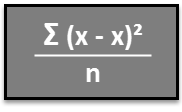
VAR uses the following formula:

where x is the sample mean AVERAGE(number1,number2,…) and n is the sample size.

Example
Copy the example data in the following table, and paste it in cell A1 of a new Excel worksheet. For formulas to show results, select them, press F2, and then press Enter. If you need to, you can adjust the column widths to see all the data.
|
Strength |
||
|
1345 |
||
|
1301 |
||
|
1368 |
||
|
1322 |
||
|
1310 |
||
|
1370 |
||
|
1318 |
||
|
1350 |
||
|
1303 |
||
|
1299 |
||
|
Formula |
Description |
Result |
|
=VAR(A2:A11) |
Variance for the breaking strength of the tools tested. |
754.2667 |
Need more help?
Want more options?
Explore subscription benefits, browse training courses, learn how to secure your device, and more.
Communities help you ask and answer questions, give feedback, and hear from experts with rich knowledge.
Excel Variance (Table of Contents)
- Introduction to Variance in Excel
- How to Calculate Variance in Excel?
Introduction to Variance in Excel
Variance is used in cases if we have some budgets, and we may know the variances observed in implementing the budgets. In some cases, the term variance is also used to calculate the difference between the planned and the actual results. Variance calculation is a great way for data analysis as this let us know the spread through of variation in the data set.
Variance is nothing but just information that shows us how well the data is spread through. Calculating variance is required, especially in cases where we have been doing a sampling of data. This is important because we use the correct function to calculate the variance like VAR.S or VAR.P. We have a few cases to calculate variance in excel where we have some data that has been projected for the period, and we want to compare that with the actual figures.
How to Calculate Variance in Excel?
Let’s understand how to Calculate Variance in Excel with some examples.
You can download this Variance Excel Template here – Variance Excel Template
Example #1 – Calculating variance in excel for the entire population
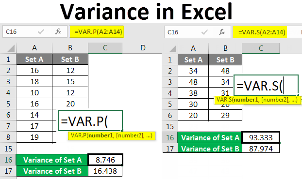
If the data set is for the complete population, then we need to use the VAR.P function of excel. This is because, in excel, we have two functions that are designed for different datasets.
We may have data that is collected based on sampling, which might be the population of the entire world.
VAR.P uses the following formula:
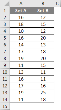
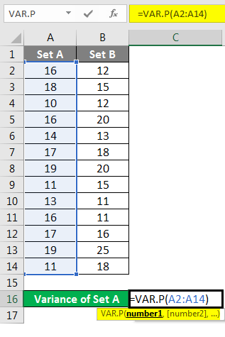
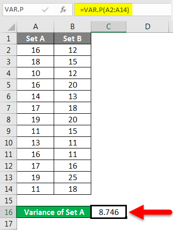
Step 1 – Enter the data set in the columns.
Step 2 – Insert the VAR.P function and choose the range of the data set. Here one thing should be noted that if any cell has an error, then that cell will be ignored.
Step 3 – After pressing the Enter key, we will get the variance.
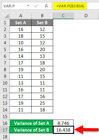
We have calculated the variance of Set B by following the same steps given above. The result of the variance of Set B is shown below.
Example #2 – Calculating the variance for sample size in excel
If we have data set that represents samples, then we need to use the function of VAR.S instead of using the VAR.P
This is because this function has been designed to calculate the variance, keeping in mind the sampling method’s characteristics.
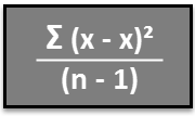
VAR.S uses the following formula:
Step 1 – Enter the data set in the column.
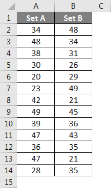
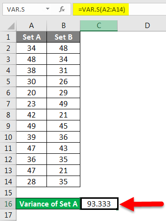
Step 2 – Insert the VAR.S function and choose the range of the data set.
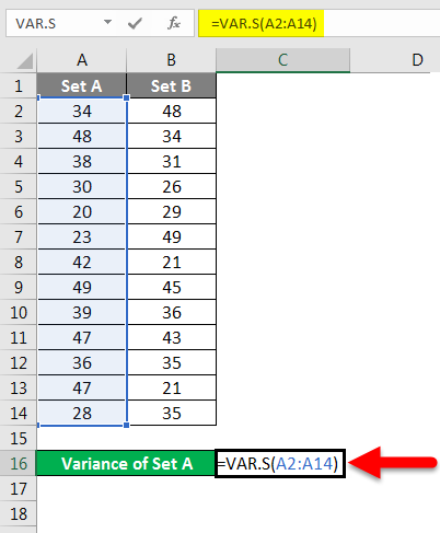
Step 3 – We will get the variance.
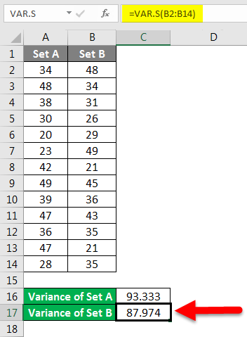
We have calculated the variance of Set B by following the same steps given above. The result of the variance of Set B is shown below.
Example #3 – Calculating the quantum of variance for data in excel
We may just want to calculate the variance in the data, and we may need the variance in terms of quantity and not in terms of data analysis.
If we need to check the change, then we need to use the following method.
Step 1 – Calculate the difference that is between the two of the data by using the function of subtraction.
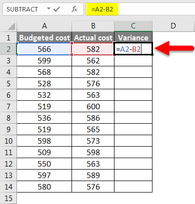
Step 2 – After pressing the Enter key, we will get the result. To get the entire data variance, we have to drag the formula applied to cell C2.
Step 3 – Now, the variance can be positive and negative, and this will be the calculated variance.
Example #4 – Calculating the percentage of variance for the data set in excel
We may need to calculate the percentage change in the data over a period of time, and in such cases, we need to use the below method.
Step 1 – First, calculate the variance from method 3rd.
Step 2 – Now calculate the percentage by using the below function.
Change in the value/original value*100. This will be our percentage change in the data set.
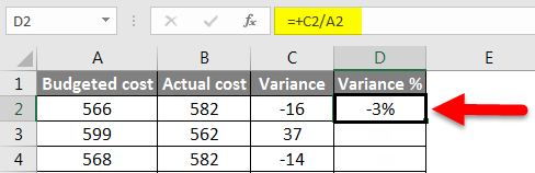
Step 3 – To get the percentage of the entire data variance, we have to drag the formula applied to cell D2.
Things to Remember About Variance in Excel
- If we have data set that represents the complete population, then we need to use the function of VAR.P.
- If we have a data set that represents the samples from the world data, then we need to use the function of VAR.S.
- Here S represents the samples.
- If we are calculating the change in terms of quantum, then a negative change means an increase in actual value and a positive change means a decrease in value.
- In the case of using the VAR.P, the arguments can be number or name, arrays or reference that contains numbers.
- If any of the cells that have been given as a reference in the formula contains an error, then that cell will be ignored.
Recommended Articles
This is a guide to Variance in Excel. Here we discussed How to calculate Variance in Excel along with practical examples and a downloadable excel template. You can also go through our other suggested articles –
- Top 25 Useful Advanced Excel Formulas and Functions
- FLOOR Function in Excel
- Excel Square Root Function
- Excel Variance
133
133 people found this article helpful
Find the spread of your data using variance and standard deviation
Updated on December 8, 2022
What to Know
- Use the VAR.P function. The syntax is: VAR.P(number1,[number2],…)
- To calculate standard deviation based on the entire population given as arguments, use the STDEV.P function.
This article explains data summarization and how to use deviation and variance formulas in Excel for Microsoft 365, Excel 2019, 2016, 2013, 2010, 2007, and Excel Online.
Summarizing Data: Central Tendency and Spread
The central tendency tells you where the middle of the data is, or the average value. Some standard measures of the central tendency include the mean, the median, and the mode.
The spread of data means how much individual results differ from the average. The most straightforward measure of spread is the range, but it’s not very useful because it tends to keep increasing as you sample more data. Variance and standard deviation are much better measures of spread. The variance is simply the standard deviation squared.
A sample of data is often summarized using two statistics: its average value and a measure of how spread out it is. Variance and standard deviation are both measures of how spread out it is. Several functions let you calculate variance in Excel. Below, we’ll explain how to decide which one to use and how to find variance in Excel.
Standard Deviation and Variance Formula
Both the standard deviation and the variance mesure how far, on average, each data point is from the mean.
If you were calculating them by hand, you would start by finding the mean for all your data. You would then find the difference between each observation and the mean, square all those differences, add them all together, then divide by the number of observation.
Doing so would give the variance, a kind of average for all the squared differences. Taking the variance’s square root corrects the fact that all the differences were squared, resulting in the standard deviation. You will use it to measure the spread of data. If this is confusing, don’t worry. Excel does the actual calculations.
Sample or Population?
Often your data will be a sample taken from some larger population. You want to use that sample to estimate the variance or standard deviation for the population as a whole. In this case, instead of dividing by the number of observation (n), you divide by n-1. These two different types of calculation have different functions in Excel:
- Functions with P: Gives the standard deviation for the actual values you have entered. They assume your data is the whole population (dividing by n).
- Functions with an S: Gives the standard deviation for a whole population, assuming your data is a sample taken from it (dividing by n-1). It can be confusing, as this formula provides the estimated variance for the population; the S indicates the dataset is a sample, but the result is for the population.
Using the Standard Deviation Formula in Excel
To calculate the standard deviation in Excel, follow these steps.
-
Enter your data into Excel. Before you can use the statistics functions in Excel, you need to have all your data in an Excel range: a column, a row, or a group matrix of columns and rows. You need to be able to select all the data without selecting any other values.
For the rest of this example, the data is in the range A1:A20.
-
If your data represents the entire population, enter the formula «=STDEV.P(A1:A20).» Alternatively, if your data is a sample from some larger population, enter the formula «=STDEV(A1:A20).»
If you’re using Excel 2007 or earlier, or you want your file to be compatible with these versions, the formulas are «=STDEVP(A1:A20),» if your data is the entire population; «=STDEV(A1:A20),» if your data is a sample from a larger population.
-
The standard deviation will be displayed in the cell.
How to Calculate Variance in Excel
Calculating variance is very similar to calculating standard deviation.
-
Ensure your data is in a single range of cells in Excel.
-
If your data represents the entire population, enter the formula «=VAR.P(A1:A20).» Alternatively, if your data is a sample from some larger population, enter the formula «=VAR.S(A1:A20).»
If you’re using Excel 2007 or earlier, or you want your file to be compatible with these versions, the formulas are: «=VARP(A1:A20),» if your data is the entire population, or «=VAR(A1:A20),» if your data is a sample from a larger population.
-
The variance for your data will be displayed in the cell.
FAQ
-
How do I find the coefficient of variation in Excel?
There’s no built-in formula, but you can calculate the coefficient of variation in a data set by dividing the standard deviation by the mean.
-
How do I use the STDEV function in Excel?
The STDEV and STDEV.S functions provide an estimate of a set of data’s standard deviation. The syntax for STDEV is =STDEV(number1, [number2],…). The syntax for STDEV.S is =STDEV.S(number1,[number2],…).
Thanks for letting us know!
Get the Latest Tech News Delivered Every Day
Subscribe
Variance is a statistical measurement that measures the spread between data points in a data set. It is defined mathematically as the average of the squared deviations from the mean. The formula for sample variance and populations variance is


where x is a data point, x bar is the mean of the data points in the data set, and n is the number of data points in the data set.
We can calculate variance in Excel both using the mathematical formula and built-in functions.
Using the Variance Mathematical Formula in Excel
Let us consider a sample data set containing integer values for which variance is sought.

First, we need to calculate the mean of the numbers as the mean is a parameter in the formula for variance. To calculate the mean in Excel, we use an in-built AVERAGE function. The syntax of the AVERAGE function is =AVERAGE(start cell reference:end cell reference). Follow these steps to calculate the mean in Excel:
- Select the cell where you want to display the mean.
- Type the formula =AVERAGE( and select the data range containing the values for which mean value is sought.
- Finish the formula with ). Here, the numbers are present in cells from A2 to A11, so we type =AVERAGE(A2:A11) in the formula bar.

- Press the Enter key to calculate and display the result.

Now that we have calculated the mean, we need to calculate the deviation of individual data points from the mean. The deviations are calculated in the column right next to the data points. Follow these steps to calculate the deviations:
- Select the cell right next to the first data point. In this example, this cell is B2.
- To get the difference, type =A2-$B$13, the $ sign makes the value constant.

- Press the Enter key to display the result.

- Simply copy the formula for the entire list to calculate the deviation for every data point by dragging down the fill handle.

Next, we need to calculate the squares of the deviations. This can be calculated using the caret operator ^. Follow these steps to find the squares of the deviations in the column next to it:
- Select the cell right next to the first deviation. In this example, this cell is C2.
- To get the square, type =B2^2 in the formula bar.

- Press the Enter key to display the result.

- Simply copy the formula for the entire list to calculate the square of deviation for every data point by dragging down the fill handle.

We now need to calculate the sum of the square of deviations. We can do this by using an inbuilt function SUM in Excel. Follow these steps to calculate the sum of all deviations:
- Go to the cell where you want to display the sum.
- Type the formula =SUM( and select the data range containing the values for which summation value is sought.
- Finish the formula with ). Here, the deviations are present in cells from C2 to C11, so we type =SUM(C2:C11) in the formula bar.

- Press the Enter key to display the calculated sum.

Sample variance is the sum of squares of deviations divided by (n -1), where n is the number of data points in the sample. Follow these steps to calculate the variance of the sample:
- Go to the cell where you want to display the variance.
- Type =B14/(10-1), where B14 contains the sum of squares of deviations.

- Press the Enter key to display the calculated result.

Population variance is the sum of squares of deviations divided by n, where n is the number of data points in the sample. Follow these steps to calculate the variance of the population:
- Go to the cell where you want to display the variance.
- Type =B14/10, where B14 contains the sum of squares of deviations.

- Press the Enter key to display the calculated result.

Using the VAR.S and VAR.P function
In Excel, an inbuilt function VAR.S calculates variance based on a sample. Syntax: VAR.S(n), where n is the list of numbers or reference to the cell ranges containing the numbers.
- Select the cell where you want to display the sample variance.
- Type the formula =VAR.S( and select the data range containing the values for which sample variance is sought.
- Finish the formula with ). Here, the numbers are present in cells from A2 to A11, so we type =VAR.S(A2:A11) in the formula bar.

- Press the Enter key to display the calculated result.

Note: The VAR.S function ignores logical values and text in the sample.
In Excel, an inbuilt function VAR.P calculates variance based on the entire population. Syntax: VAR.P(n), where n is the list of numbers or reference to the cell ranges containing the numbers.
- Select the cell where you want to display the population variance.
- Type the formula =VAR.P( and select the data range containing the values for which population variance is sought.
- Finish the formula with ). Here, the numbers are present in cells from A2 to A11, so we type =VAR.P(A2:A11) in the formula bar.

- Press the enter key to display the calculated result.

Note: The VAR.P function ignores logical values and text in the sample.
Conclusion
In this tutorial, we learned how to calculate sample and population variance both by using mathematical formulas and inbuilt functions VAR.S and VAR.P in Excel.
Содержание
- Вычисление дисперсии
- Способ 1: расчет по генеральной совокупности
- Способ 2: расчет по выборке
- Вопросы и ответы

Среди множества показателей, которые применяются в статистике, нужно выделить расчет дисперсии. Следует отметить, что выполнение вручную данного вычисления – довольно утомительное занятие. К счастью, в приложении Excel имеются функции, позволяющие автоматизировать процедуру расчета. Выясним алгоритм работы с этими инструментами.
Вычисление дисперсии
Дисперсия – это показатель вариации, который представляет собой средний квадрат отклонений от математического ожидания. Таким образом, он выражает разброс чисел относительно среднего значения. Вычисление дисперсии может проводиться как по генеральной совокупности, так и по выборочной.
Способ 1: расчет по генеральной совокупности
Для расчета данного показателя в Excel по генеральной совокупности применяется функция ДИСП.Г. Синтаксис этого выражения имеет следующий вид:
=ДИСП.Г(Число1;Число2;…)
Всего может быть применено от 1 до 255 аргументов. В качестве аргументов могут выступать, как числовые значения, так и ссылки на ячейки, в которых они содержатся.
Посмотрим, как вычислить это значение для диапазона с числовыми данными.
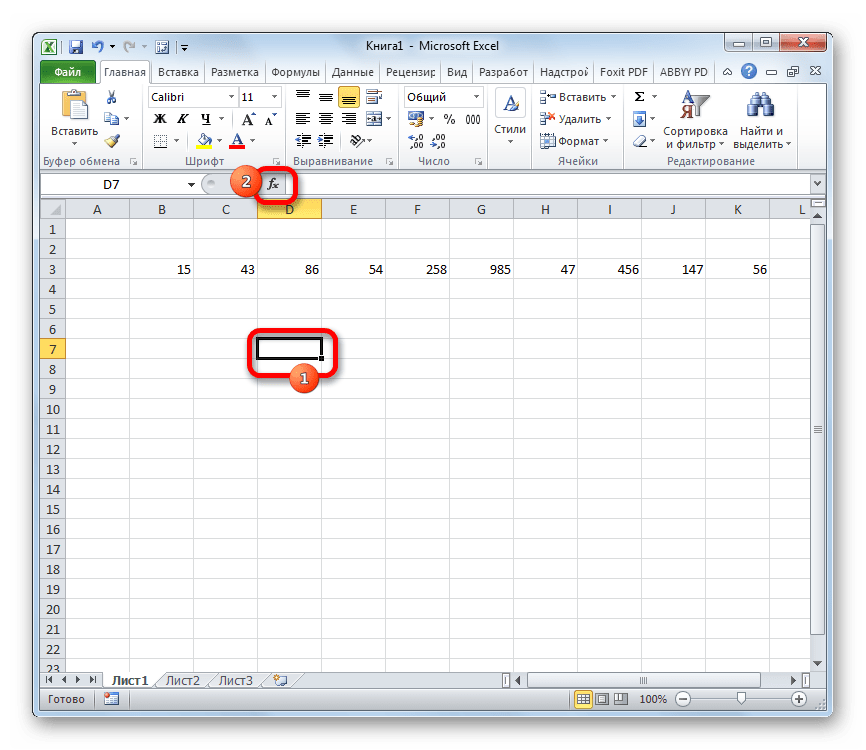
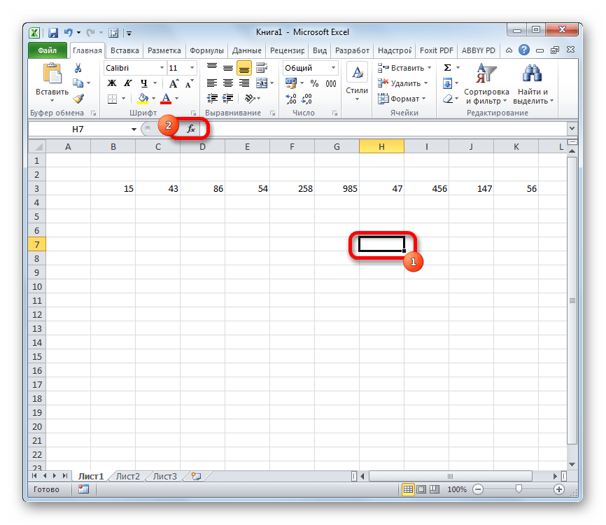
- Производим выделение ячейки на листе, в которую будут выводиться итоги вычисления дисперсии. Щелкаем по кнопке «Вставить функцию», размещенную слева от строки формул.
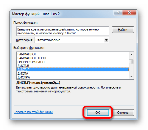
- Запускается Мастер функций. В категории «Статистические» или «Полный алфавитный перечень» выполняем поиск аргумента с наименованием «ДИСП.Г». После того, как нашли, выделяем его и щелкаем по кнопке «OK».
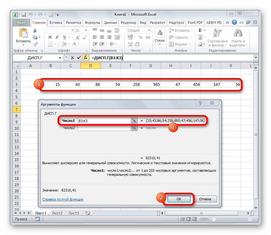
- Выполняется запуск окна аргументов функции ДИСП.Г. Устанавливаем курсор в поле «Число1». Выделяем на листе диапазон ячеек, в котором содержится числовой ряд. Если таких диапазонов несколько, то можно также использовать для занесения их координат в окно аргументов поля «Число2», «Число3» и т.д. После того, как все данные внесены, жмем на кнопку «OK».
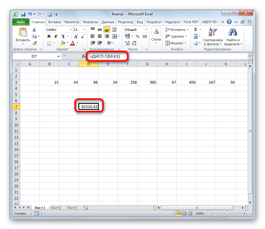
- Как видим, после этих действий производится расчет. Итог вычисления величины дисперсии по генеральной совокупности выводится в предварительно указанную ячейку. Это именно та ячейка, в которой непосредственно находится формула ДИСП.Г.
Урок: Мастер функций в Эксель
Способ 2: расчет по выборке
В отличие от вычисления значения по генеральной совокупности, в расчете по выборке в знаменателе указывается не общее количество чисел, а на одно меньше. Это делается в целях коррекции погрешности. Эксель учитывает данный нюанс в специальной функции, которая предназначена для данного вида вычисления – ДИСП.В. Её синтаксис представлен следующей формулой:
=ДИСП.В(Число1;Число2;…)
Количество аргументов, как и в предыдущей функции, тоже может колебаться от 1 до 255.

- Выделяем ячейку и таким же способом, как и в предыдущий раз, запускаем Мастер функций.
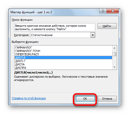
- В категории «Полный алфавитный перечень» или «Статистические» ищем наименование «ДИСП.В». После того, как формула найдена, выделяем её и делаем клик по кнопке «OK».
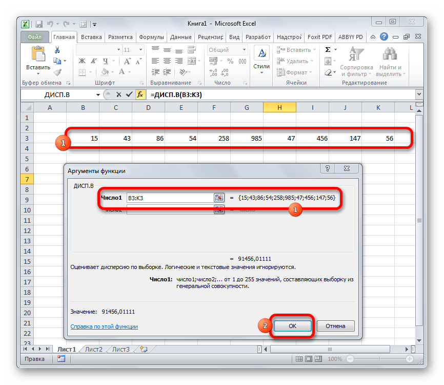
- Производится запуск окна аргументов функции. Далее поступаем полностью аналогичным образом, как и при использовании предыдущего оператора: устанавливаем курсор в поле аргумента «Число1» и выделяем область, содержащую числовой ряд, на листе. Затем щелкаем по кнопке «OK».
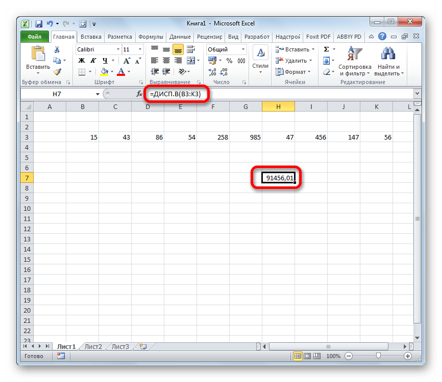
- Результат вычисления будет выведен в отдельную ячейку.
Урок: Другие статистические функции в Эксель
Как видим, программа Эксель способна в значительной мере облегчить расчет дисперсии. Эта статистическая величина может быть рассчитана приложением, как по генеральной совокупности, так и по выборке. При этом все действия пользователя фактически сводятся только к указанию диапазона обрабатываемых чисел, а основную работу Excel делает сам. Безусловно, это сэкономит значительное количество времени пользователей.
Еще статьи по данной теме: