Variance analysis with excel

The variance method is used to analyze the variance of an attribute under the influence of controlled variables.

The factor method suits for examining the connections between values. Let’s consider the analytic tools in detail: namely, the factor, variance and two-factor variance methods for assessing the variability.



Variance Analysis In Excel

In conventional terms, the objective of the variance method is as follows: to single out three particular variances from the general variance of a parameter:

• the variance determined by the influence of each of the values under consideration;
• the variance dictated by the interconnection between the values under consideration;
• the random variance dictated by all the unconsidered circumstances.

Microsoft Excel allows for performing the variance analysis with the help of the tool «Data Analysis» (the tab «DATA» — «Analysis»). It’s a customization plugin of the spreadsheet processor. If the plugin is unavailable, go to «Excel Options» and enable the analysis tool.

The work starts with executing the table. The rules are:

1. Each column should contain a value of one of the factors under consideration.
2. The columns should be organized in ascending/descending order of the value of the parameter under consideration.

Let’s review an example of variance analysis in Excel.

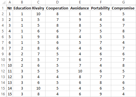
Using a dedicated method, the company’s psychologist has analyzed the behavior strategies of employees in a conflict situation. It is assumed that the behavior is influenced by the subject’s education level (1 stands for secondary, 2 for vocational, 3 for higher).

Enter the data into the Excel table:

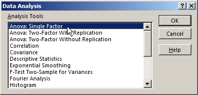
1. Open the dialog window of the analytic tool. Select «Anova: Single Factor» in the list and click OK.



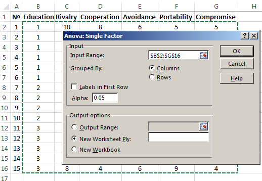
2. In the «Input Range» field, enter the link to the range of cells contained in all the table columns $B$2:$G$16.



3. Select «Grouped By»-«Columns».
4. Select «New Worksheet Ply:» in the «Output options:». If you need to indicate the output range within the existing spreadsheet, switch it to the « Output Range:» and enter the link to the top left cell of the range for the output data. The size of the range will be determined automatically.
5. The analysis results are output on a separate spreadsheet (in our example).

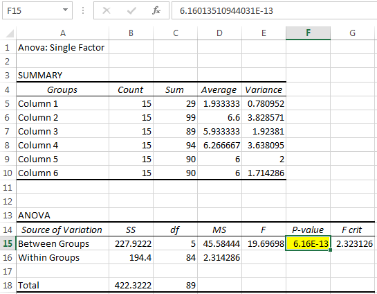
The parameter of importance is filled-in with yellow. As the P value between the groups exceeds 1, Fisher’s variance ratio cannot be considered of importance. Consequently, the behavior in a conflict situation does not depend on the subject’s education level.



Factor Analysis In Excel: An Example

Factor analysis is a multi-variance analysis of the inter-connections between the values of the variables. This method allows to resolve some very important tasks:

• to describe the object under observation in a comprehensive yet concise manner;
• to reveal the hidden variable values that determine the presence of linear statistical correlations;
• to classify the variables (determining the inter-connections between them);
• to reduce the number of the necessary variables.

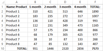
Let’s review an example of conducting a factor analysis. Let’s assume we know the data regarding the sales of certain goods during the past 4 months. We need to analyze which items are in demand and which are non-demanded.

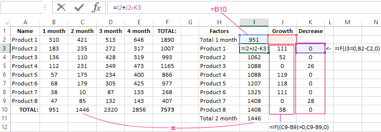
1. Let’s find out which items ensured the main part of the growth in the second month. If the sales of a certain kind of goods grew, the positive delta goes to the «Growth» column. Negative deltas go to «Decrease». For «Growth», the Excel formula is: =IF((C2-B2)>0,C2-B2,0), where С2-В2 is the difference between the 2nd and 1st months. For «Decrease», the formula is: =IF(J3=0,B2-C2,0), where J3 is the link to the left cell («Growth»). The second column will contain the sum of the previous value and the previous growth, deducting the current decline.



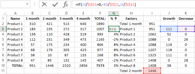
2. Let’s calculate the growth percentage for each item. The formula is: =IF(J3/$I$11=0,-K3/$I$11,J3/$I$11). Here, J3/$I$11 stands for the ratio between the «Growth» and the result of the 2nd month. ;-K3/$I$11 stands for the ratio between the «Decrease» and the result of the 2nd month.



3. Select the range of data for building the chart. Go to the tab «INSERT»-«Chart».



4. Let’s adjust the legend and the colors. Remove the cumulative total through «Format Data Series» — «FILL» («No fill»). Use this tool to change the colors for «Decrease» and «Growth».

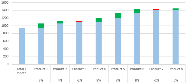
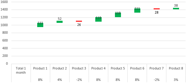
Now we have a visual demonstration of which kinds of goods ensured the main part of the sales growth.

Two-Factor Variance Analysis In Excel

This method demonstrates the influence of two factors on the variance of a random variable’s value. Let’s consider an example of performing the two-factor variance analysis in Excel.

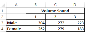
Problem. A group of men and women were demonstrated sounds of various volumes: 1 – 10dB, 2 – 30dB, 3 – 50dB. The response time was recorded in milliseconds. It’s necessary to determine: whether or not the subject’s sex influences the response time; whether or not the volume influences the response time.

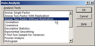
1. Go to the tab «DATA»-«Data Analysis». Select «Anova: Two-Factor Without Replication» from the list.



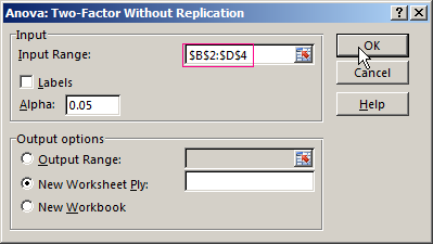
2. Fill in the fields. Only numeric values should be included in the range.



3. The analysis result should be output on a new spreadsheet (as was set).

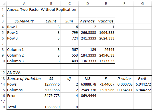
Since the F statistics (the «F» column) for the «gender» factor exceeds the critical level of the F distribution (the column «F-critical »), this factor does have an impact on the parameter under analysis (the time of response to the sound).

As another example, the factor analysis of the deviations in marginal income is provided below:

Download Factor and Variance analysis example

Download analysis example 2

For the «Volume Sound» factor: 2,9 < 6,94. Consequently, this factor has no influence on the response time.

Most companies create plans and budgets to establish benchmarks for future performance in sales, production, operations, labor, etc. The starting point of these plans and budget are usually estimated cost and revenue figures. The goal is to meet these budgets, but as with all goals — they are not always met. Managers use variance analysis to track the actual performance against these goals. If this analysis is not performed afterwards, then setting budgets is useless.

In other words: after a period (i.e. month, quarter, year) is over, managers, management accountants, controllers and other finance professionals calculate (and then analyze) a number of different types of variance. Variance is defined as the difference between the actual values (costs, revenue, head count, …) and budgeted, planned or standard values.

Favorable and adverse variance

After a variance is calculated, it falls into one of these two categories:

1. Favorable variance (positive; better than planned)
2. Adverse variance (negative; worse than planned)

An example of a favorable variance is when actual total costs are lower than the planned total costs. An example of an adverse variance is when the actual revenue is lower than planned.

Note: not all adverse variance is bad and not all favorable variance is good! For example, a variance analysis might show higher production costs than planned (adverse variance). However, a deeper look reveals that the higher costs are a direct consequence of significantly higher sales (favorable variance).

How to perform variance analysis?

There are a couple of different ways to perform variance analysis. Excel spreadsheets are still the most widely used tool for it, so we’ll use them in our examples as well. Additionally, here’s how to master variance visualization in Power BI if you’d rather do it there.

Here are three examples of variance reports:

1. The Classic Sales-vs-Plan or Costs-vs-Plan Report

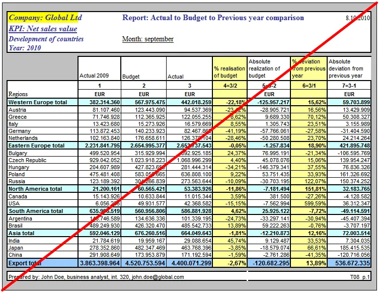
In this most common example, you’d have the planned (or budget) values in one column, the actual values in another column, and the variance in the third column. Add some additional columns for good measure, spice it up with some color and you soon end up with an illegible mess like this:

A much better way to display the variances is using plus-minus variance charts. Following this advice, we can use Zebra BI Tables for Office to present the above data in this way in Excel:

Every variance should provoke questions. Why did we perform poorly in Western Europe and Bulgaria? Is this negative variance a change in plans, an execution failure, an advertising campaign gone wrong, or a certain move from one of the competitors, or was the budget unrealistic at the start?

The answers to questions like these should be written on the report itself (using a couple of short comments as you see above). Variance reports are often poorly designed; turn yours into a clean, easy-to-read report in 8 simple steps.

Without this data and without these answers, the management can’t make the right decisions for the future of the company. They will ask the question why anyway, so it’s better to include the answer right from the start.

Do you want to create a sales variance report like the one in the second image? Download a free template, simply change the demo data with your own and start looking for business insights.

Note: The data in the above report represents sales. If we report on costs, the red/green colors in the charts must be inverted. Lower costs than planned is a good thing (green), higher costs is bad (red).

2. Direct comparison of categories: actual vs. previous year

If we have a flat structure (without subtotals), a good way to compare the elements is to use integrated variance charts. They display the actual values as bars (or columns) while the absolute variances are integrated into the bars (or columns) themselves.

We can also add Zebra BI lollipop charts to display relative variances. Of course, don’t forget to write a descriptive title and comments!

3. Forecasting: year-to-date monthly variance with end-of-year forecast

When it comes to forecasting in variance reports, management is mainly interested in two things:

1. how we’re doing so far in the current year and
2. are we on track to meet our yearly goals.

To visualize this we use the same type of report as above, but divide it into two parts.

The left part is the year-to-date part where we display the actual results compared to the budget. This part is about the past.

The right part is about the future. Here we compare the approved yearly budget with the latest forecast. These are end-of-year (EoY) figures and the variance chart in between shows whether according to the latest estimation we will meet the annual plan or not for each data element (in our case for each account manager):

Note: Because we’re comparing forecast vs. budget and not actual vs. budget, the bars in the right-hand chart are visualized differently. The IBCS recommends a diagonal-striped pattern fill (automatically applied by Zebra BI).

The above variance report serves as an indicator of our performance against the yearly plan. The two-part nature of the report gives management a look at the recent past — The company’s cumulative results from the start of the year — as well as a view into the future — how the company is expected to perform until the end of the year. Equipped with this data, they can make the correct decisions.

To take things one step further, we can add the actual figures from the current month. Our report now consists of three parts:

1. current month performance,
2. year-to-date performance and
3. full year forecast

Need a differently structured report? Explore more best practice variance analysis report templates for Excel.

The limitations and shortcomings of variance analysis

Here are some of the problems of variance analysis that companies must be aware of:

• Time delay. The analysts typically calculate and analyze the variances at the end of each period and then report the results to the management. In a fast-paced environment (like manufacturing etc.), management needs feedback much faster than once a month, and tends to rely upon measurements and warnings that are produced on the spot.
• Effort required. In order for analysts to really do their job well, they must dig deep to find the underlying causes for the variances. This includes sorting through a lot of different sources of information. The extra work if only cost-effective when management is capable of acting accordingly to fix the issues.
• Setting budgets. Since variance analysis is essentially comparing actual results with planned ones, it is necessary that these plans were sound in the first place. If they are a result of using some arbitrary standards, political bargaining or even blindly relying on data from previous periods, they are actually of very little use.

The solution to these problems is to use trend analysis in conjunction with variance analysis. In trend analysis, the results of multiple periods are listed side by side, making it easy to detect trends. Also consider a Price Volume Mix analysis to improve your understanding of your business.

Remember: Although variance analysis can become very complex, the main guide is always common sense. Yes, lower actual costs than planned is a positive variance, and higher costs than planned is a negative variance. But the real question that needs to be answered is whether or not the result was good for business.

Want to insert charts like these in your variance analysis reports with Zebra BI for Office?

The new Zebra BI for Office lets you visualize your data with just one click. This way you can get to the right business insights faster and spend more time on making the correct business decisions.

Выполним детерминированный факторный анализ на примере модели, описывающей связь финансовых показателей предприятия. Рассмотрим наиболее общий способ цепных подстановок. Для проведения факторного анализа используем надстройку

MS

EXCEL

Variance

Analysis

Tool

от компании

Fincontrollex

.

Для выполнения

детерминированного факторного анализа

в среде MS EXCEL сначала кратко напомним читателям о самом методе, затем покажем, как провести

факторный анализ

самостоятельно на примере простой однопродуктовой модели, и наконец, воспользуемся специализированной надстройкой

Variance

Analysis

Tool

для более сложной многопродуктовой модели

.

Немного теории

Сначала дадим сухое академическое определение

факторного анализа

, затем поясним его на примерах.

Детерминированный факторный анализ (ДФА)

— это методика исследования влияния

факторов

на

результативный показатель

. Предполагается, что связь

факторов

с

результативным показателем

носит функциональный характер, которая  выражена математической формулой.

Приведем пример такой функциональной связи. В качестве результативного показателя возьмем

выручку

предприятия, а в качестве факторов, влияющих на выручку –

объем продаж

,

цену реализации изделия

и

наценку

, учитывающая срок оплаты (чем позже покупатель оплатил товар, тем выше наценка). Формула функциональной связи в этом случае выглядит так:

Выручка=(Объем продаж изделия за период)*(Цена изделия)*Наценка

Эта формула является моделью, т.е. разумным упрощением реальности. Действительно, в этой модели есть ряд очевидных допущений:

• предприятие выпускает единственный продукт;
• предполагается, что цена на изделие не меняется в течение периода исследования (на самом деле часто цена зависит от условий поставок различным потребителям);
• у предприятия нет других источников выручки кроме продаж изделия (например, отсутствуют доходы от внереализационных операций);
• под выручкой подразумевается валовая выручка, а не чистая (за вычетом НДС, скидок) и т.д.

Примечание

:

Детерминированный анализ

исключает любую неопределенность и случайность, присутствующие в процессе реальной деятельности предприятия. Хотя результаты такого анализа являются приблизительными, но они помогают исследователю определить степень влияния факторов на результирующий показатель и часто являются отправной точкой для проведения более детального анализа.

Примечание

: Представленная выше модель является

мультипликативной

, т.е. чтобы получить

результирующий показатель

необходимо перемножить факторы. Также имеются

аддитивные

(Результат=Фактор1+Фактор2+…),

кратные

(Результат=Фактор1/Фактор2) и

смешанные модели

(Результат=Фактор1*Фактор2+Фактор3).

Для проведения ДФА нам понадобятся 2 набора значений факторов и соответствующих им результирующих показателей. Часто в качестве первого набора (называемого базовым) выбирают плановые значения, а в качестве второго – фактические.

Для нашей

мультипликативной

модели

Выручка=Объем*Цена*Наценка

заполним следующую таблицу с плановыми и фактическими значениями:

Как видно из таблицы, фактическая выручка существенно меньше плановой. Это произошло из-за того, что фактические значения всех факторов получились меньше запланированных. Необходимо проанализировать, какой фактор внес наибольший вклад в снижение результата:

Цена, Наценка

или

Объем продаж

.

В

детерминированном факторном анализе

используют следующие способы анализа:

• способ цепных подстановок;
• способ абсолютных разниц;
• способ относительных (процентных) разниц;
• интегральный метод и др.

Воспользуемся наиболее универсальным

способом цепных подстановок

, который может использоваться во всех типах моделей –

аддитивных, мультипликативных, кратных

и

смешанных

.

Способ цепных подстановок

позволяет выявить, какие факторы повлияли на результирующий показатель наиболее значительно. Этот способ заключается в следующем:

• Сначала изменяют значение одного фактора с планового на фактическое (в нашем случае изменим
  
  Объем продаж
  
  ). При этом другие факторы (
  
  Цену
  
  и
  
  Наценку
  
  ) нужно оставить неизменными (плановой). Затем вычисляют результирующий показатель (
  
  Выручку
  
  ), а результат сравнивают с имеющимся предыдущим значением (с плановой
  
  Выручкой
  
  ). Далее находят их разность. Чем больше разность по абсолютной величине, тем больше влияние данного фактора на показатель.
• На втором шаге изменяют значения сразу двух факторов на их фактические значения (
  
  Объем
  
  и
  
  Цену
  
  ), при этом остальные факторы (
  
  Наценку
  
  ) оставляют неизменными (плановыми). Далее вычисляют результирующий показатель (
  
  Выручку
  
  ), и сравнивают его со значением, полученным на предыдущем шаге.
• Далее повторяют замену значений факторов с плановых на фактические до тех пор, пока не будут заменены значения всех факторов модели на фактические.

Все вышесказанное можно записать с помощью простых математических выражений.

Сделаем это на примере

3-х факторной

мультипликативной

модели).

Начинаем с формулы, содержащей только плановые значения факторов:

Результат(План) = Фактор1(План) *Фактор2(План) *Фактор3(План)

Затем для всех факторов по очереди подставляем их фактические значения вместо плановых.

Результат(1)= Фактор1(Факт) *Фактор2(План) *Фактор3(План)

Результат(2)= Фактор1(Факт) *Фактор2(Факт) *Фактор3(План)

Результат(3)= Фактор1(Факт) *Фактор2(Факт) *Фактор3(Факт)

Примечание

:

Результат(3) = Результат(Факт),

т.е. значению результирующего показателя с фактическими значениями всех факторов

.

При этом общее изменение Результата будет равно:

Δ Результат = Результат(Факт) – Результат(План)

С другой стороны, общее изменение Результата складывается из суммы изменений результирующего показателя за счет изменения каждого фактора:

Δ Результат = Δ Результат(1) + Δ Результат(2) + Δ Результат(3)

При этом,

Δ Результат(1) = Результат(1) – Результат(План)

Δ Результат(2) = Результат(2) – Результат(1)

Δ Результат(3) = Результат(Факт) – Результат(2)

И наконец, определим значение Δ

Результат(

i

),

которое будет максимальным по

абсолютной величине. Соответствующий фактор (i) и будет являться фактором, наиболее повлиявшим на результирующий показатель.

Проведем

детерминированный факторный анализ

для

мультипликативной модели

способом

цепных подстановок

в случае одного изделия в среде MS EXCEL. Все вычисления сделаем с помощью обычных формул.

Вычисления в MS EXCEL

В соответствии с вышеуказанным алгоритмом произведем расчеты

способом цепных постановок

. Для этого рассчитаем значения выручки, последовательно заменяя значения факторов с плановых на фактические (

см. файл примера, лист ДФА

).

Далее, вычислим влияние каждого фактора на результат, оставляя значения остальных факторов неизменными:

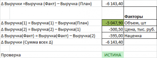
С помощью правила

Условного форматирования

=ABS($M11)=МАКС(ABS($M$11:$M$13))

выделим значение, которое привело к максимальному отклонению результирующего показателя. В нашем случае это значение соответствует фактору

Объем продаж

.

Очевидно, что в случае

мультипликативной модели

, фактор, который претерпел наибольшее относительное изменение, всегда будет являться фактором, ответственным за максимальное отклонение результирующего показателя.

В этом можно непосредственно убедиться, проведя анализ изменений факторов модели:

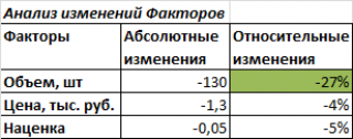
Такой результат будет очевидным только при использовании модели для анализа предприятия выпускающего одно изделие. Если предприятие выпускает несколько изделий, которые продаются по разным ценам и с различными наценками, то расчеты для детерминированного факторного анализа значительно усложняются.

К счастью, имеются специализированные программы для проведения

факторного анализа

. Так как среда MS EXCEL является гибким и одновременно мощным средством для проведения расчетов, то для сложных моделей рекомендуем использовать надстройку

Variance

Analysis

Tool

от компании

Fincontrollex

.

Сначала покажем, как быстро освоить эту надстройку, а затем произведем вычисления на примере

смешанной модели

в случае многопродуктовой стратегии предприятия.

Надстройка Variance Analysis Tool

Скачать надстройку можно с сайта

http://fincontrollex.com

, выбрав ее в меню

Продукты

или соответствующую иконку на главной странице сайта.

На сайте также можно найти подробную справку к надстройке и очень полезный видеоурок (

http://fincontrollex.com/?page=products&id=3&lang=ru

).

На странице продукта нажмите кнопку «Скачать бесплатно». Надстройка будет скачана на компьютер в формате архива zip. В архиве содержится 2 файла надстройки *.xll: x64 – для 64 и x86 – для 32 – разрядной версии MS EXCEL. Чтобы узнать версию вашей программы в меню

Файл

выберите пункт

Справка

.

После установки надстройки появится новая вкладка fincontrollex.com.

К надстройке вернемся чуть позже, сейчас создадим

смешанную модель

и заполним исходную таблицу с плановыми и фактическими значениями для факторов и результирующего показателя.

Создание модели

Рассмотрим более сложную модель выручки предприятия, зависящую от 3-х факторов:

Выручка=СУММ(Объем продаж изделия(

i

)*(Цена за 1 шт. изделия(

i

))+бонус(

i

))

Как видно из формулы предприятие теперь продает несколько изделий, причем каждое изделие имеет свою цену. За своевременную оплату поставленной партии клиенту может быть начислен бонус (скидка): если платеж осуществлен в течение первых 3-х дней после отгрузки (поставки), то бонус составляет 20 000 руб. за партию; если оплата поступила не позже недели, то бонус составит 10 000 руб., если позже, то бонус не начисляется.

Составим исходную таблицу для плановых и фактических значений:

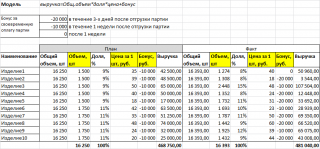
Заголовки столбцов таблицы, содержащие значения, которые вводятся пользователем, выделены желтым цветом. Остальные числовые ячейки содержат формулы (

см. файл примера, лист Таблица

).

Руководители предприятия, очевидно, планировали продать изделия с артикулом с 1 по 5 в количестве по 1500 шт., а остальные изделия по 1750 шт. Фактические объемы продаж по некоторым позициям существенно отличаются. Также отличается и цена, по которой менеджеры по продажам договорились реализовать изделия. Наличие бонуса сыграло свою роль при оплате и большинство клиентов оплатили товар вовремя или даже ранее срока, которые прогнозировали руководители (от 3-х дней до 1 недели).

Но, какой из факторов оказал большее влияние на выручку? Кого из сотрудников нужно премировать: руководство, которое придумало систему Бонусов; менеджеров по продажам, которые договорились о цене и объемах каждого изделия или производственный отдел, которые обеспечили гибкое изготовление партий (существенно отличающееся по объемам от планового). Ответ далеко не очевиден.

Как было показано в предыдущем разделе, для проведения

факторного анализа

можно самостоятельно написать формулы. Однако, очевидно, что даже для однопродуктовой модели это достаточно трудоемко, и, следовательно, легко можно допустить вычислительную ошибку.

Чтобы этого не произошло – разумно воспользоваться специальной надстройкой

Variance

Analysis

Tool

.

Расчет с помощью надстройки Variance Analysis Tool

Итак, у нас есть модель (формула) и таблица с исходными данными. Чтобы воспользоваться надстройкой нам потребуется немного изменить нашу формулу:

Выручка=СУММ(Объем продаж изделия(

i

)*(Цена за 1 шт. изделия(

i

)) +бонус(

i

))

Для того, чтобы понять зачем нам придется менять казалось бы разумную формулу, рассмотрим более детально фактор

Объем продаж изделия

.

Очевидно, что важен как

суммарный объем продаж

(в штуках), так и

ассортимент изделий

. Можно получить рост суммарного объема продаж, но при этом потерять в выручке за счет снижения продаж более дорогих изделий, чем было запланировано. Например, менеджеры запланировали продать 2 товара по 100 шт. каждого. Один товар стоит 10 руб., другой 50 руб. Плановая выручка должна была составить 6000 руб.=100*10+100*50. Фактически же удалось продать 250 шт.: 200шт. по 10 руб. и 50 шт. по 50 руб. В итоге имеем снижение выручки до 4500 руб.!

Прелесть в том, что при правильном написании формулы с помощью

факторного анализа

можно определить влияние на выручку обоих факторов: отдельно определить влияние общего, т.е.

суммарного объема продаж

, а также влияние проданного

ассортимента

изделий.

Таким образом, фактор

Объем продаж изделия

, который мы использовали в однопродуктовой модели, в случае продаж нескольких изделий требуется разделить на 2 составляющих: на

Общий объем продаж

и на

Долю продаж каждого изделия

. Следовательно, наша модель превращается из 3-х факторной в 4-х факторную.

Примечание

: На сайте fincontrollex.com можно прочитать статью про

факторный анализ выручки

(

http://fincontrollex.com/?page=articles&id=6&lang=ru

), в которой подробно изложен материал о том, как учесть влияние различных каналов продаж продукции, оценить эффект от ввода новых продуктов, определить влияние скидок и учесть эффекты от других управленческих инициатив.

Новая формула, учитывающая влияние

ассортимента

и

общего объема продаж

на выручку, выглядит так:

Выручка=Общий объем продаж*СУММ(Доля продаж изделия(

i

)*(Цена за 1 шт. изделия(

i

)))+ СУММ(бонус(

i

))

Или более кратко:

Выручка=Общ.объем*Доля*Цена+Бонус

Теперь настроим модель.

Во вкладке fincontrollex.com нажмите кнопку

Выполнить

.

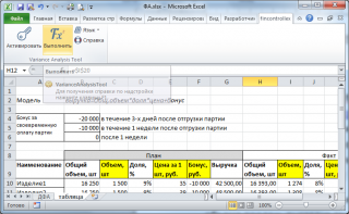
Появится диалоговое окно надстройки

Variance

Analysis

Tool

.

Введите название модели (произвольный текст) и формулу модели.

Формула модели не должна содержать точек (.), но может содержать пробелы. После ввода формулы нажмите клавишу ENTER (ВВОД) или кликните на кнопку

Параметры модели

или в поле

Название модели

.

Названия факторов в формуле не обязательно должны совпадать с названиями столбцов исходной таблицы. Соответствие между формулой и исходной таблицей устанавливаются с помощью ссылок (см. ниже).

После ввода формулы надстройка автоматически определит тип модели (смешанная) и факторы, одновременно создав перечень факторов из формулы в столбце

Наименование

в нижней части окна.

В поле

Диапазон названий

нужно ввести ссылку на наименования изделий.

Чтобы связать факторы, указанные в формуле с соответствующими данными из исходной таблицы, необходимо обязательно заполнить 3 столбца:

• В столбце
  
  Описание
  
  нужно ввести ссылки на названия колонок факторов из исходной таблицы;
• В столбце
  
  Базовый
  
  диапазон
  
  нужно ввести ссылки на соответствующие ячейки с плановыми значениями факторов;
• В столбце
  
  Фактический диапазон
  
  нужно ввести ссылки на соответствующие ячейки с фактическими значениями факторов;

Столбец

Ед.изм.

имеет информативный характер и может содержать единицы измерения факторов. На вычисления этот столбец не влияет и его в принципе можно не заполнять (по крайней мере, при отладке модели расчета).

Осталось нажать кнопку меню

Выполнить

, и тем самым запустить расчет.

Расчет выполняется практически мгновенно. После выполнения расчета создается новая книга с 2-мя листами:

Свод

и

Подробно

.

Показатель

База

на листе

Свод

равен в нашем случае плановой выручке, а

Факт

– фактической выручке. Между ними расположены все 4 фактора модели. По значениям этих факторов можно быстро определить влияние этих факторов на результирующий показатель (выручку).

Очевидно, что факторы

Цена

и

Бонус

оказали практически одинаковое воздействие на выручку, но с противоположным знаком. Таким образом, менеджеры по продажам могут надеяться на премию, т.к. им удалось добиться существенного повышения цены и, соответственно, обеспечив самый значительный дополнительный вклад в выручку по сравнению с плановым. Также был правильно подобран ассортимент изделий (+7210 у фактора

Доля

). Это означает, что было продано больше дорогих изделий, чем дешевых по сравнению с планом.

На листе

Подробно

можно увидеть детальный расчет с формулами.

В сфере финансового анализа ничего нельзя принимать на веру, поэтому нами были внимательно изучены формулы, которые генерирует надстройка, а алгоритм их работы был сверен с теорией.

Очевидно, что надстройка

Variance

Analysis

Tool

хорошо справилась со своим «предназначением», все расчеты произведены верно и что очень важно – быстро.

Освоение надстройки не занимает много времени. После просмотра видеоурока (10 минут) любой пользователь MS EXCEL сможет начать работу с надстройкой, построить модель и выполнить

детерминированный факторный анализ способом цепных подстановок

.

Вывод

: Сайт

www.excel2.ru

рекомендует финансовым аналитикам и менеджерам использовать надстройку

Variance Analysis Tool

от Fincontrollex для выполнения

детерминированного факторного анализа

моделей самых разнообразных видов.

Содержание

• Вычисление дисперсии
  • Способ 1: расчет по генеральной совокупности
  • Способ 2: расчет по выборке
• Вопросы и ответы

Среди множества показателей, которые применяются в статистике, нужно выделить расчет дисперсии. Следует отметить, что выполнение вручную данного вычисления – довольно утомительное занятие. К счастью, в приложении Excel имеются функции, позволяющие автоматизировать процедуру расчета. Выясним алгоритм работы с этими инструментами.

Вычисление дисперсии

Дисперсия – это показатель вариации, который представляет собой средний квадрат отклонений от математического ожидания. Таким образом, он выражает разброс чисел относительно среднего значения. Вычисление дисперсии может проводиться как по генеральной совокупности, так и по выборочной.

Способ 1: расчет по генеральной совокупности

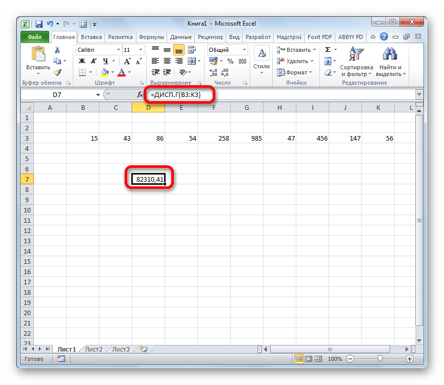
Для расчета данного показателя в Excel по генеральной совокупности применяется функция ДИСП.Г. Синтаксис этого выражения имеет следующий вид:

=ДИСП.Г(Число1;Число2;…)

Всего может быть применено от 1 до 255 аргументов. В качестве аргументов могут выступать, как числовые значения, так и ссылки на ячейки, в которых они содержатся.

Посмотрим, как вычислить это значение для диапазона с числовыми данными.

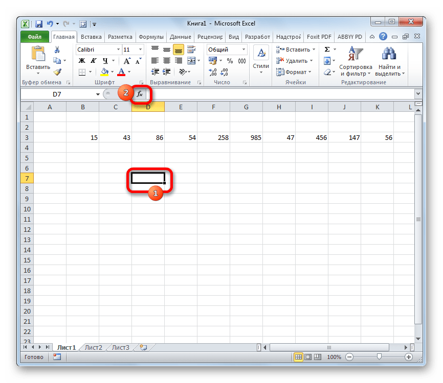
1. Производим выделение ячейки на листе, в которую будут выводиться итоги вычисления дисперсии. Щелкаем по кнопке «Вставить функцию», размещенную слева от строки формул.



2. Запускается Мастер функций. В категории «Статистические» или «Полный алфавитный перечень» выполняем поиск аргумента с наименованием «ДИСП.Г». После того, как нашли, выделяем его и щелкаем по кнопке «OK».



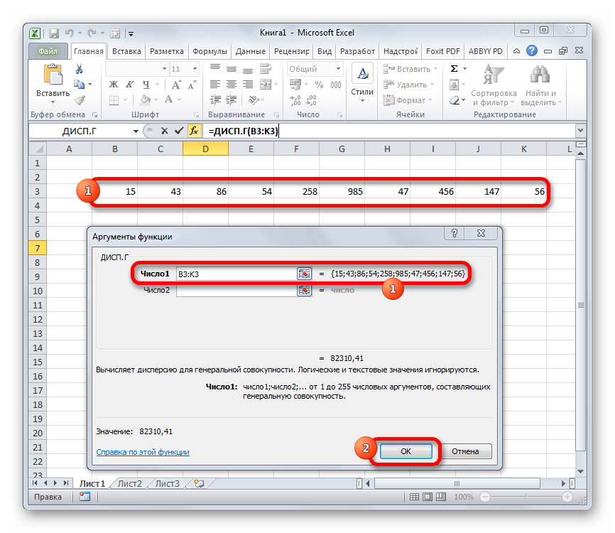
3. Выполняется запуск окна аргументов функции ДИСП.Г. Устанавливаем курсор в поле «Число1». Выделяем на листе диапазон ячеек, в котором содержится числовой ряд. Если таких диапазонов несколько, то можно также использовать для занесения их координат в окно аргументов поля «Число2», «Число3» и т.д. После того, как все данные внесены, жмем на кнопку «OK».



4. Как видим, после этих действий производится расчет. Итог вычисления величины дисперсии по генеральной совокупности выводится в предварительно указанную ячейку. Это именно та ячейка, в которой непосредственно находится формула ДИСП.Г.

Урок: Мастер функций в Эксель

Способ 2: расчет по выборке

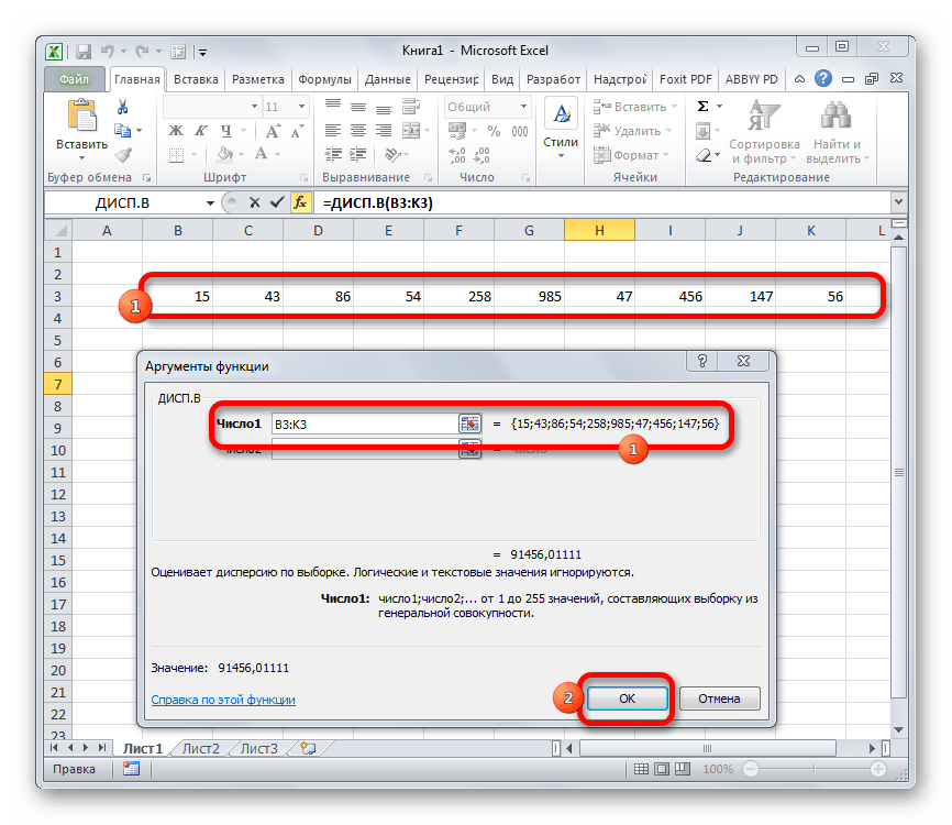
В отличие от вычисления значения по генеральной совокупности, в расчете по выборке в знаменателе указывается не общее количество чисел, а на одно меньше. Это делается в целях коррекции погрешности. Эксель учитывает данный нюанс в специальной функции, которая предназначена для данного вида вычисления – ДИСП.В. Её синтаксис представлен следующей формулой:

=ДИСП.В(Число1;Число2;…)

Количество аргументов, как и в предыдущей функции, тоже может колебаться от 1 до 255.

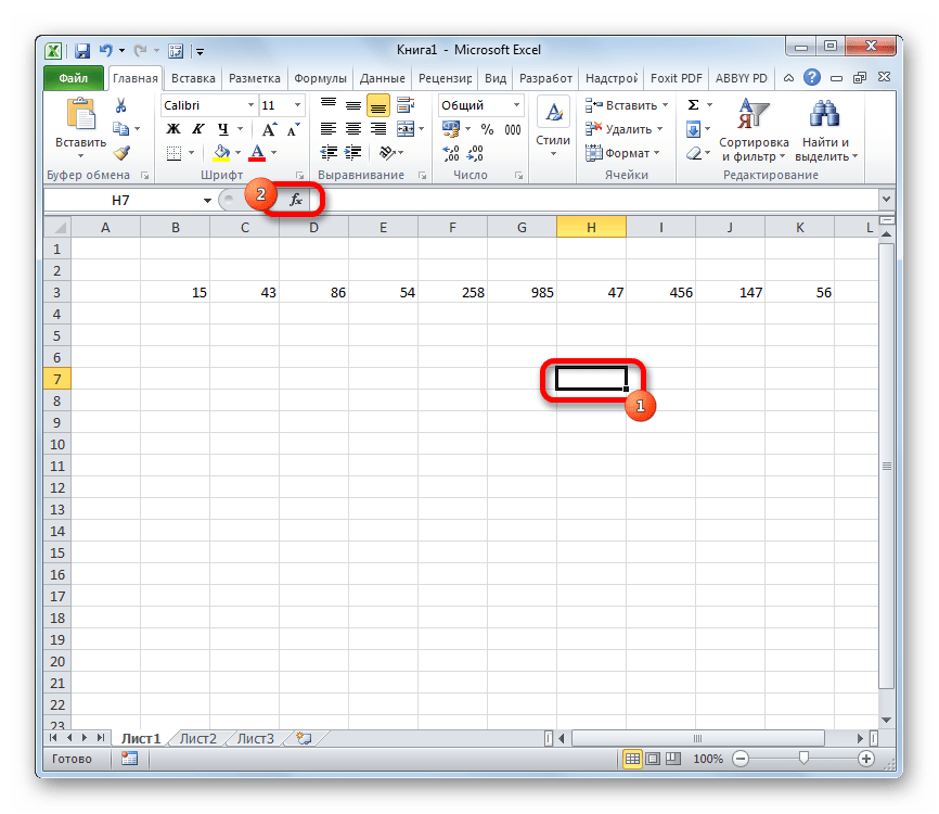
1. Выделяем ячейку и таким же способом, как и в предыдущий раз, запускаем Мастер функций.



2. В категории «Полный алфавитный перечень» или «Статистические» ищем наименование «ДИСП.В». После того, как формула найдена, выделяем её и делаем клик по кнопке «OK».



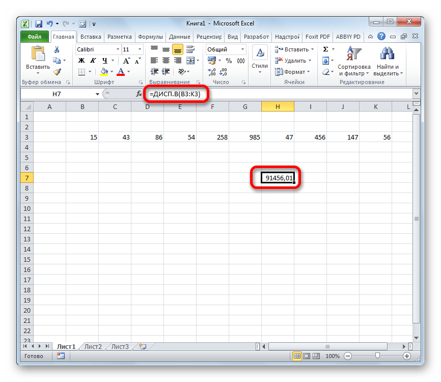
3. Производится запуск окна аргументов функции. Далее поступаем полностью аналогичным образом, как и при использовании предыдущего оператора: устанавливаем курсор в поле аргумента «Число1» и выделяем область, содержащую числовой ряд, на листе. Затем щелкаем по кнопке «OK».



4. Результат вычисления будет выведен в отдельную ячейку.

Урок: Другие статистические функции в Эксель

Как видим, программа Эксель способна в значительной мере облегчить расчет дисперсии. Эта статистическая величина может быть рассчитана приложением, как по генеральной совокупности, так и по выборке. При этом все действия пользователя фактически сводятся только к указанию диапазона обрабатываемых чисел, а основную работу Excel делает сам. Безусловно, это сэкономит значительное количество времени пользователей.

Еще статьи по данной теме:

Помогла ли Вам статья?

Whether it is daily life thing or any day at work, we are always comparing to see whats good and what is not so good. This differential analysis has a much popular name as variance analysis.

Whenever, whatever and whoever is deciding, you got to have the variance report to better understand the situation and what control actions are needed. Read this if you are interested in details about What is Variance analysis?

Normally this is how variance analysis looks like:

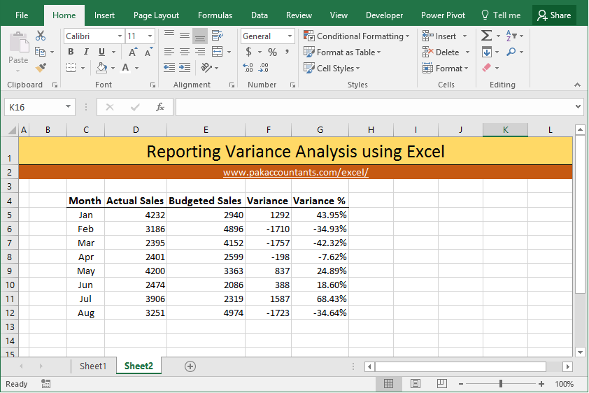Not much a of a fan like this… right?

Lets face it! when you are in the seat deciding things you would like to have the data in such shape that you can process with most of your organs and senses and not just brain. That is why colors, charts and mix of other things are used. Following are 10 techniques to take variance analysis beyond simple numbers and percentages.

Method 1 Use brackets for negative numbers

Simplest of all and very formal too. At the moment that small dash at left for negative or unfavourable variance need an effort in itself to see. Putting numbers in brackets make it much easier on eyes to separate the good from bad. This is how to do it:

Select the cells you want to format > hit Ctrl+1 on the keyboard > from the dialogue box select number tab > select custom from the list at left > Under type input box remove anything that is written and put this:

0;(0);0

Click OK and now you have negative numbers in brackets.

With percentages the format code will be a little different as following:

0.00%;(0.00)%;0%

If you are one of those souls who pursue finesse at every level then you can adjust the format a little more for percentages so that numbers and brackets don’t break the visual harmony of the report. Lets change the code as following and see what it does:

0.00_)%;(0.00)%;0_)%

With negative numbers enclosed in brackets, the digit’s position is shifted a little and can cause confusion. Adding “_)” element helps get it sorted. See we are adding it only to positive number and zero portion of the code.

Method 2 Color the content or data – Custom number format

We can even use colors to differentiate the negative numbers/percentages from positive ones in addition to brackets or on simple numbers.

Again, go to custom number format dialogue box by selecting the data and hitting Ctrl+1 and put this code for numbers:

[Blue]0;[Red]0;0

This will give positive numbers in blue color, negative numbers in red and 0 will remain default color.

You can even use colors with the code mentioned in method 1 above as follows:

[Blue]0_);[Red](0);0_)

This code will show positive numbers in blue and negative numbers in brackets with red color while keeping the column aligned nicely.

So what we did is basically add color codes in square brackets for each of the positive and negative number portion of the code. You can use other specific color codes as well or apply a color only to negative or positive number.

Method 3 Use arrows

We can use up and down arrows to show the positive and negative numbers or favourable and unfavourable variance.

The basic trick is to input character code using number pad while holding down the ALT key on the keyboard. Yes! you need number pad for this. Number keys above alphabet keys won’t work.

Select the data and go to custom number format dialogue box by hitting Ctrl+1 combo. Go to custom and remove anything from type input bar. Press “0” key followed by a tap of spacebar and then press + hold down ALT key and from number pad press 3 followed by 0. Let go of ALT key and an arrow up will be inserted! Or simply ALT + 3 + 0.

Same goes for negative number but this time instead of 3 and 0, press 3 and 1 and it will insert an arrow down. So for arrow down the combination is ALT + 3 + 1

As wordpress won’t allow me to paste the original code so I am just putting the structure of code as following:

0 [space] [arrow up];0 [space] [arrow down];0

One improvement that can make it better by having arrows aligned to the right of the cell and numbers to the left of the cell. This is done by adding one additional element which is esterisk. So the structure will be as following:

0[esterisk][space][arrow up];0[esterisk][space][arrow down];0

As you can see we are including only esterisk symbol before the space character to the same code discussed earlier.

And definitely you can use colors as well to give more oomph:

Method 4 Use cell color

If you are not fond of colored text then you can use cell color to change for negative and/or positive numbers.

Select the data > go to home tab > styles group > click conditional formatting drop down button > click new rule. From the dialogue box select “Use a formula to determine which cells to format”

Now we can put a formula to color the cells with negative numbers with a simple formula like this one:

=G5<0

Click format button and select the color of cell you desire and make other formatting related changes if you want. Once done click OK to apply the conditional formatting.

Method 5 Use arrows – Conditional formatting

We saw how to use arrows to differential positive and negative figures using custom number formatting in method 3 above, but you can do very similar thing using conditional formatting as well.

Go to home tab > styles group > click conditional formatting drop down button > click new rule. Having the first rule type selected, change format style to icon sets. Change to icon style of your choice which in our case is arrows. From the type drop down change the value to “Numbers” for both. Have the first condition as “>” 0 and second condition has “>=” 0 and click OK.

Method 6 Use data bars

One my favourite way to present variances with great visual impact that adds a lot to understanding and the best part is its super quick to implement.

Select the data > go to home tab > styles group > click conditional formatting drop down button > data bars > select the style you like. Done!

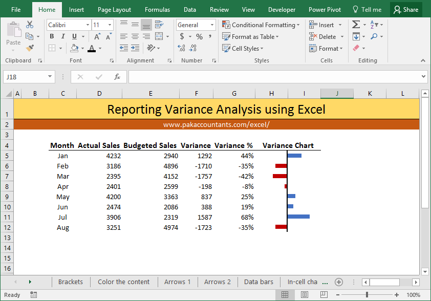
Method 7 “In-cell” charts

So far we have been utilizing builtin features of Excel. Like databars that do really good job, but there is limited control. Another alternative is to make in cell charts using REPT function with symbols.

I have already explained this technique in great detail here: Budget vs Actual Variance Reports with “In the Cell Charts” in Excel

This technique requires two columns as we will be “plotting” negative and positive numbers separately. I will be using “|” called pipe or vertical bar. You can use any other symbol you like but this is the most easily accessible right from your keyboard.

So we will we use two columns, left one for negative figures and right for positive figures.

As my data is in G column and I am using percentage figures to make the in cell graph, so I will use the following formulas:

Negative number column:

=IF(G5<0,REPT("|",ROUND(ABS(G5)*100,0)),"")

Positive number column:

=IF(G5>0,REPT("|",ROUND(ABS(G5)*100,0)),"")

Select the cells and double click the fill handle to populate through whole range. Now we need to do a little formatting. Select the negative graph column and make it right-aligned. Select both columns and change the font to “Stencil”. Give negative column red color and positive blue or any that you like.

If you you don’t hav “Stencil” installed then you can use “Britanica Bold” or “Playbill” just to do the same.

If you think chart is taking too much space then you can adjust the size of font or change the multiplicative factor of “100” in formula to 50 or any lower number. For best understanding have the width of both columns equal. 

Following is another variation of the same technique:

This chart is included in the downloadable bundle

Method 8 Use scaled-down actual charts

Well this is definitely an option no denying in that. But best part is that you can scale them down to fit just like in-cell charts. I really like scaled down charts as they do really good in excel dashboards.

Select the data meaning only numbers or percentage whatever you want to use as base data for chart. Go to Insert tab > charts group > click column or bar chart drop down button > click stacked bar chart.

Chart will be inserted. We need to make few formatting changes like getting rid of legends, title, bottom axis scale adjustment and later deleting it, and hiding the series labels using custom number format option to be left with bare bars!

Following animation walks you through the whole process:

In my case the values are plotted as last value first. To correct this we can choose the “reverse order” option.

Now the values are plotted in the right order and also on the correct side of the chart i.e. positive values on the right side and negative on the left.

Here is another variation achieved with a little clever application of the same technique:

This chart is included in the downloadable bundle

Method 9 Make better variance charts

Have a look at it first:

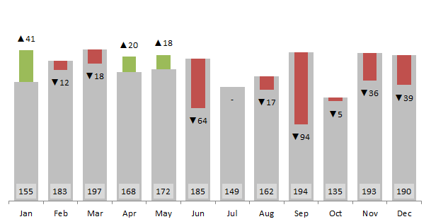
Lovely isn’t it! Want to make it? I have discussed its construction in probably the most detailed tutorial till date here: Variance Analysis in Excel – Making better Budget Vs Actual charts

Give it a read. The tutorial is not just about one variance analysis chart but a lot of other techniques that go into making it. One notable one is dynamic data labels

This chart is included in the downloadable bundle

Method 10 Highlight instances in chart

Probably the most interesting of all of the above. This is basically a chart but designed in a way that positive values are plotted with different color and negative values are plotted with another.

In addition to this, I have added On/Off switch so that if someone wants to highlight only negative or positive figures then it can be done easily.

To learn the technique head over to this tutorial: Highlight instances in Excel charts in different colors with shaded bars in background

This chart is included in the downloadable bundle

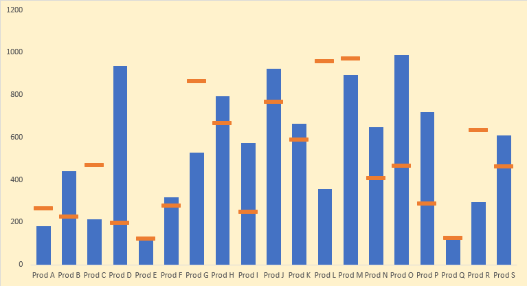
Method 11: Awesome Actual vs target variance charts

This advanced variance analysis chart does more in less space with amazing clarity to present actual and budgeted or targeted results in one Excel chart. To learn how to make this chart head over to this detailed tutorial.

This chart is included in the downloadable bundle

Method 12: Actual vs target variance charts with floating bars

In this quick and easy tutorial you will learn how to make a variance analysis chart in less than 60 seconds that is not just functional but beautiful to look at as well. To learn this specific chart head over to this page to read the tutorial.

This chart is included in the downloadable bundle

Method 13: Top to bottom vertical variance analysis with bar charts

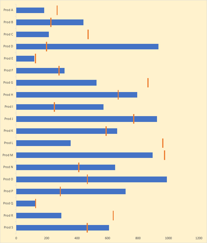
With advancement in tools we use to manage and communicate, our screen orientation has taken complete 90 degree change and this is where this charting technique comes handy. Instead of having your cell phone in landscape orientation and still missing the bits, you can keep the cell phone in natural portrait orientation and easily scroll up or down for even longer charts.

Also you will learn a fine technique to have floating bars using ONLY bar charts. This nifty technique is a must learn!

This chart is included in the downloadable bundle

So here is my list of 10+ ways to report variances so far. I would love to add more to it! But first let me know how do you like to report variances in your report in the comment section and if you have a technique with an x-factor then I would love to read about it!