
Return to Excel Formulas List
Download Example Workbook
Download the example workbook
This tutorial demonstrates how to get a cell value using the address of the cell (row and column) in Excel and Google Sheets.
Get Cell Value With the INDEX Function
We can get the value of a cell (its content) by using the INDEX Function.
The INDEX Function looks up a cell contained within a specified range and returns its value.
=INDEX(A1:J10,C3,C4)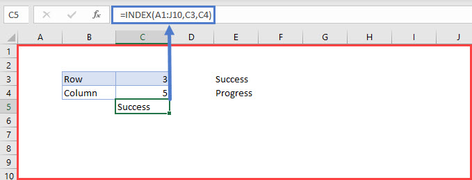
In the example above, the range specified in the INDEX formula is “A1:J10”, the row is cell “C3” (“3”), and the column is cell “C4” (“5”).
The formula looks through the range “A1:J10”, checks the cell in Row 3 and Column 5 (“E3”) and returns its value (“Success”).
Get Cell Value With the INDIRECT Function
Another option for getting the value of a cell by its address is to use the INDIRECT Function.
We can use the INDIRECT Function here in two different ways.
Using Text Reference Within the INDIRECT Function
The INDIRECT Function changes a specified text string to a cell reference and returns its value.
=INDIRECT("R" & 3 & "C" & 2,FALSE)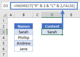
In the example above, the specified text string is “R3C2”. This means Row 3, Column 2. So the formula returns the value in that address (“Sarah”).
Note: The FALSE argument in this formula indicates the cell reference format (R1C1). (TRUE would use A1 style cell referencing).
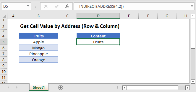
Get Cell Value by Using INDIRECT and ADDRESS
The second way to get the value of a cell using the INDIRECT Function is to combine it with the ADDRESS Function.
=INDIRECT(ADDRESS(4,2))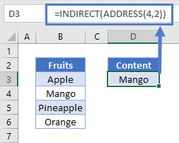
Let’s breakdown the formula into steps.
=ADDRESS(4,2)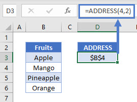
The ADDRESS Function takes a specified row number (“4”) and column number (“2”) and returns its absolute reference (“$B$4”). Therefore, the absolute reference for the cell in Column 2 (Column B based on position) and Row 4 is $B$4.
The INDIRECT Function returns the value of the cell referenced.
=INDIRECT(D3)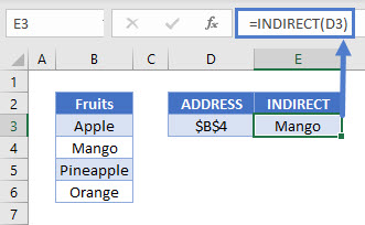
Combining these steps gives us our initial formula:
=INDIRECT(ADDRESS(4,2))
Note: The INDIRECT Function is volatile. It recalculates every time the workbook does and can cause Excel to run slowly. We recommend avoiding the use of large numbers of INDIRECT Functions in your workbooks.
Get Cell Value by Address in Google Sheets
These formulas work exactly the same in Google Sheets as in Excel.
Excel for Microsoft 365 Excel for Microsoft 365 for Mac Excel for the web Excel 2021 Excel 2021 for Mac Excel 2019 Excel 2019 for Mac Excel 2016 Excel 2016 for Mac Excel 2013 Excel 2010 Excel 2007 Excel for Mac 2011 Excel Starter 2010 More…Less
This article describes the formula syntax and usage of the ADDRESS function in Microsoft Excel. Find links to information about working with mailing addresses or creating mailing labels in the See Also section.
Description
You can use the ADDRESS function to obtain the address of a cell in a worksheet, given specified row and column numbers. For example, ADDRESS(2,3) returns $C$2. As another example, ADDRESS(77,300) returns $KN$77. You can use other functions, such as the ROW and COLUMN functions, to provide the row and column number arguments for the ADDRESS function.
Syntax
ADDRESS(row_num, column_num, [abs_num], [a1], [sheet_text])
The ADDRESS function syntax has the following arguments:
-
row_num Required. A numeric value that specifies the row number to use in the cell reference.
-
column_num Required. A numeric value that specifies the column number to use in the cell reference.
-
abs_num Optional. A numeric value that specifies the type of reference to return.
|
abs_num |
Returns this type of reference |
|
1 or omitted |
Absolute |
|
2 |
Absolute row; relative column |
|
3 |
Relative row; absolute column |
|
4 |
Relative |
-
A1 Optional. A logical value that specifies the A1 or R1C1 reference style. In A1 style, columns are labeled alphabetically, and rows are labeled numerically. In R1C1 reference style, both columns and rows are labeled numerically. If the A1 argument is TRUE or omitted, the ADDRESS function returns an A1-style reference; if FALSE, the ADDRESS function returns an R1C1-style reference.
Note: To change the reference style that Excel uses, click the File tab, click Options, and then click Formulas. Under Working with formulas, select or clear the R1C1 reference style check box.
-
sheet_text Optional. A text value that specifies the name of the worksheet to be used as the external reference. For example, the formula =ADDRESS(1,1,,,»Sheet2″) returns Sheet2!$A$1. If the sheet_text argument is omitted, no sheet name is used, and the address returned by the function refers to a cell on the current sheet.
Example
Copy the example data in the following table, and paste it in cell A1 of a new Excel worksheet. For formulas to show results, select them, press F2, and then press Enter. If you need to, you can adjust the column widths to see all the data.
|
Formula |
Description |
Result |
|
=ADDRESS(2,3) |
Absolute reference |
$C$2 |
|
=ADDRESS(2,3,2) |
Absolute row; relative column |
C$2 |
|
=ADDRESS(2,3,2,FALSE) |
Absolute row; relative column in R1C1 reference style |
R2C[3] |
|
=ADDRESS(2,3,1,FALSE,»[Book1]Sheet1″) |
Absolute reference to another workbook and worksheet |
‘[Book1]Sheet1’!R2C3 |
|
=ADDRESS(2,3,1,FALSE,»EXCEL SHEET») |
Absolute reference to another worksheet |
‘EXCEL SHEET’!R2C3 |
Need more help?
When using lookup formulas in Excel (such as VLOOKUP, XLOOKUP, or INDEX/MATCH), the intent is to find the matching value and get that value (or a corresponding value in the same row/column) as the result.
But in some cases, instead of getting the value, you may want the formula to return the cell address of the value.
This could be especially useful if you have a large data set and you want to find out the exact position of the lookup formula result.
There are some functions in Excel that designed to do exactly this.
In this tutorial, I will show you how you can find and return the cell address instead of the value in Excel using simple formulas.
Lookup And Return Cell Address Using the ADDRESS Function
The ADDRESS function in Excel is meant to exactly this.
It takes the row and the column number and gives you the cell address of that specific cell.
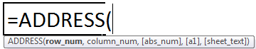
Below is the syntax of the ADDRESS function:
=ADDRESS(row_num, column_num, [abs_num], [a1], [sheet_text])
where:
- row_num: Row number of the cell for which you want the cell address
- column_num: Column number of the cell for which you want the address
- [abs_num]: Optional argument where you can specify whether want the cell reference to be absolute, relative, or mixed.
- [a1]: Optional argument where you can specify whether you want the reference in the R1C1 style or A1 style
- [sheet_text]: Optional argument where you can specify whether you want to add the sheet name along with the cell address or not
Now, let’s take an example and see how this works.
Suppose there is a dataset as shown below, where I have the Employee id, their name, and their department, and I want to quickly know the cell address that contains the department for employee id KR256.
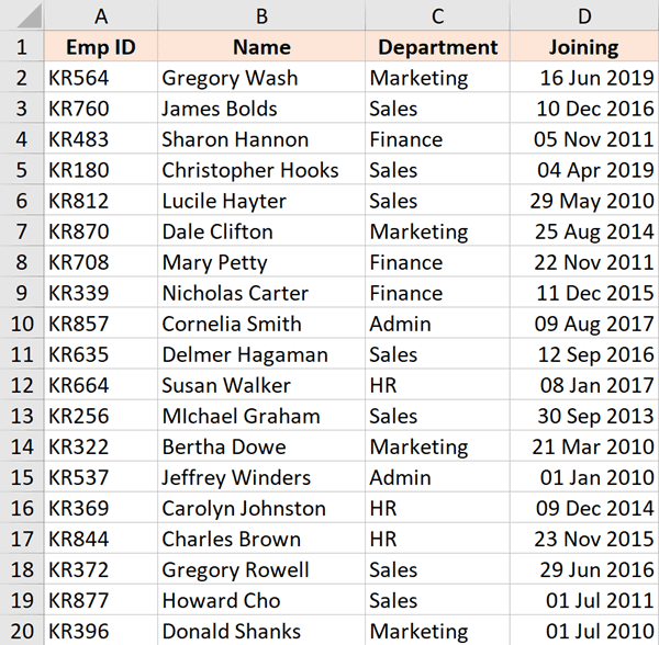
Below is the formula that will do this:
=ADDRESS(MATCH("KR256",A1:A20,0),3)
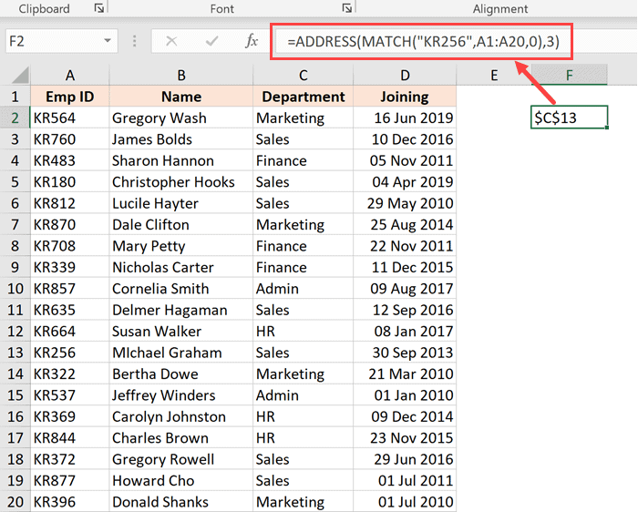
In the above formula, I have used the MATCH function to find out the row number that contains the given employee id.
And since the department is in column C, I have used 3 as the second argument.
This formula works great, but it has one drawback – it won’t work if you add the row above the dataset or a column to the left of the dataset.
This is because when I specify the second argument (the column number) as 3, it’s hard-coded and won’t change.
In case I add any column to the left of the dataset, the formula would count 3 columns from the beginning of the worksheet and not from the beginning of the dataset.
So, if you have a fixed dataset and need a simple formula, this will work fine.
But if you need this to be more fool-proof, use the one covered in the next section.
Lookup And Return Cell Address Using the CELL Function
While the ADDRESS function was made specifically to give you the cell reference of the specified row and column number, there is another function that also does this.
It’s called the CELL function (and it can give you a lot more information about the cell than the ADDRESS function).
Below is the syntax of the CELL function:
=CELL(info_type, [reference])
where:
- info_type: the information about the cell you want. This could be the address, the column number, the file name, etc.
- [reference]: Optional argument where you can specify the cell reference for which you need the cell information.
Now, let’s see an example where you can use this function to look up and get the cell reference.
Suppose you have a dataset as shown below, and you want to quickly know the cell address that contains the department for employee id KR256.
Below is the formula that will do this:
=CELL("address", INDEX($A$1:$D$20,MATCH("KR256",$A$1:$A$20,0),3))
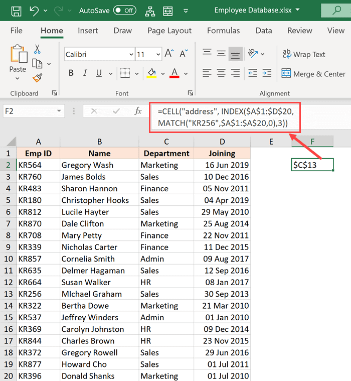
The above formula is quite straightforward.
I have used the INDEX formula as the second argument to get the department for the employee id KR256.
And then simply wrapped it within the CELL function and asked it to return the cell address of this value that I get from the INDEX formula.
Now here is the secret to why it works – the INDEX formula returns the lookup value when you give it all the necessary arguments. But at the same time, it would also return the cell reference of that resulting cell.
In our example, the INDEX formula returns “Sales” as the resulting value, but at the same time, you can also use it to give you the cell reference of that value instead of the value itself.
Normally, when you enter the INDEX formula in a cell, it returns the value because that is what it’s expected to do. But in scenarios where a cell reference is required, the INDEX formula will give you the cell reference.
In this example, that’s exactly what it does.
And the best part about using this formula is that it is not tied to the first cell in the worksheet. This means that you can select any data set (which could be anywhere in the worksheet), use the INDEX formula to do a regular look up and it would still give you the correct address.
And if you insert an additional row or column, the formula would adjust accordingly to give you the correct cell address.
So these are two simple formulas that you can use to look up and find and return the cell address instead of the value in Excel.
I hope you found this tutorial useful.
Other Excel tutorials you may also like:
- Lookup and Return Values in an Entire Row/Column in Excel
- Find the Last Occurrence of a Lookup Value a List in Excel
- Lookup the Second, the Third, or the Nth Value in Excel
- How to Reference Another Sheet or Workbook in Excel
- Lookup and Return Values in an Entire Row/Column in Excel
How to Get Cell Address in Excel (ADDRESS + CELL functions)
To obtain information about any cell in Excel, we have two functions: the CELL and the ADDRESS function.
Using these functions, you can get the address, the reference, the formula, the formatting (and much more) of a cell.
These are some of Excel’s most underrated functions, and it’s about time you learn why🤷♂️
So jump right into the guide below. And don’t forget to download our free sample workbook here as you scroll down.
How to use the ADDRESS function
The Excel ADDRESS function returns the cell address for a given row number and column letter.
It has a large but simple syntax that reads as follows:
=ADDRESS(row_num, column_num, [abs_num], [a1], [sheet_text])
In order to address the first cell (Cell A1):
- Write the ADDRESS function as follows:
=ADDRESS(1,1)
- Hit Enter to reach the following result.

The first argument represents the row number (Row 1). The second argument represents the column number (Column 1). And so the resulting ADDRESS is $A$1.
That’s all that you need – the rest of the arguments are only optional ✌
- Now write the ADDRESS function with the third argument (abs_num) set to 4.
=ADDRESS(1,1,4)
- Press Enter and here are the results:

By adding 4 as the [abs_num] argument, Excel changes our result to a relative cell reference. Something completely different from what we saw earlier.
That’s because different values for the abs_num argument return different address types.
Pro Tip!
For the [abs_num] argument:
- If you enter 1, the address type will be an absolute cell reference ($A$1).
- If you enter 2, the address type will be a mixed cell reference. (A$1 – An absolute row reference, and a relative column reference).
- If you enter 3, the address type will be a mixed cell reference. ($A1 – An absolute column reference, and a relative row reference).
- If you enter 4, the address type will be a relative cell reference (A1).
In the first example, we omitted the abs_num argument and Excel set it to 1 by default. The result was, therefore, an absolute cell reference.
But the formula doesn’t just stop here🚀
- Include the fourth argument [a1] to modify this formula further.
=ADDRESS(1,1,4,0)

Here, 0 represents the reference style.
Note that the result is in a different style from our previous example. That’s because we opted for the R1C1 reference style in which columns and rows are represented by numbers.
- To get the result in A1 reference style, add 1 as the [a1] argument :
=ADDRESS(1,1,4,1)

Note that we got the same result for our second example too.
That’s because if we omit the [a1] argument, Excel, by default, sets it to 1.
And what if you want the cell address from a different Excel sheet than the one you are currently on?
For this, you need to use the last optional argument of the ADDRESS function, i.e., [sheet_text].
It identifies the worksheet you want the cell address for 👀 Let’s try it out here:
- Write the [sheet_text] argument of the ADDRESS function as below:
=ADDRESS(1,1,4,1,”Sheet1″)

With the sheet_text argument as above, Excel generates an external reference. It returns the name of the worksheet with the cell address.
Like in the above example, Excel returns the address of the cell from Sheet 1. The Cell address is therefore prefixed by the worksheet name “Sheet1”.
If this argument is omitted, the resulting cell address won’t contain the worksheet name. And the address of the cell will be of the current sheet, by default.
How to use the CELL function
Until now we’ve seen how the ADDRESS function helps you find the address of a cell in Excel.
But what if you want to know about the location, format, formula, and content of a cell too🤔
The CELL function of Excel will help you fetch all these (and even other details about a cell). The syntax of this function reads as follows:
=CELL(info_type, [reference])
Starting with info_type, write the CELL function like this:
=CELL (
As you start writing the CELL function, Excel launches a drop-down menu of options for the argument “info_type“.

You can select from any of the 12 options in the drop-down menu above.
For example, select the option “Address” as the info_type argument. And Excel would return the address of the active (or the referred) cell.
= CELL (“Address”)

Note that we omitted the second argument of the CELL Function in the above example, i.e., [reference].
And so, the function returned the address of the active cell (Cell A2).
Pro Tip!
As the reference argument, you can refer to a single or a range of cells.
That’s not it – we still have 11 more info types to try and test.
So let’s change the arguments of our function as follows:
=CELL (“col”, A3)
Note that here we have created a reference to Cell A3 as the [reference] argument.

In this example, “col” represents the column number of cell A3 (the referred cell). The result given by Excel is 1 (the Column number for Cell A3).
Similarly, you can try different info_types to get different information about a cell. Like the following:
=CELL (“type”, A4)

“Type” returns the type of the referred cell.
Excel returned the value “B” indicating that the cell is blank. This is because we have referred to Cell A4 which is an empty string.
Pro Tip!
Under the “type” mode, if your cell contains a text constant, the result will be “I“. “B” if the cell is blank and “V” if the cell has any other data type.
The CELL function offers a wide variety of info types that you might fetch for a cell. Here’s a short tabular summary of them all 👇

The format info_type returns the format of the referred cell. It gives different results for different cells which are in the form of codes.
The image below shows a list of some common format codes along with their meanings and results. This should help clear out any confusion 🔍

That’s it – Now what?
In the above guide, we learned how to use two of the least-known yet very useful functions of Excel – the CELL and the ADDRESS function.
Finding information about a cell is no more a difficult task – thanks to the CELL function.
The ADDRESS function is also an excellent tool when used the right way. But it’s not the only one. Excel has a wide variety of functions that are equally or even more useful💪
To mention a few, the VLOOKUP, SUMIF, and IF functions of Excel. Register for my 30-minute free email course to master these right away.
Other resources
If you enjoyed reading this article, we bet you’d love to read our other blogs too. There’s certainly a lot more to learn about cell addresses and references in Excel.
Like how to use the ROW function to find the row number in Excel. Or how to use the COLUMN function to find the column number in Excel.
Kasper Langmann2023-02-23T11:17:47+00:00
Page load link
The ADDRESS function returns the absolute address of the cell based on a specified row and column number. The cell address is returned as a text string. For example, “=ADDRESS(1,2)” returns “$B$1.” An inbuilt function of Excel, it is categorized under the lookup and reference functions.
Table of contents
- Address Function in Excel
- Syntax of the ADDRESS Function
- How to Use the Address Function in Excel? (With Example)
- How to Use the INDIRECT Function to Pass the Address?
- Frequently Asked Questions
- Recommended Articles
Syntax of the ADDRESS Function
The syntax is stated as follows:
You are free to use this image on your website, templates, etc, Please provide us with an attribution linkArticle Link to be Hyperlinked
For eg:
Source: Address Function in Excel (wallstreetmojo.com)
The function accepts the following mandatory arguments:
- Row_Num: This is the row number used in the cell reference. The “row_num=1” represents row 1.
- Column_Num: This is the column number used in the cell reference. The “column_num= 2” represents column B.
The function accepts the following optional arguments:
- Abs_num (absolute number): This is the type of cell referenceCell reference in excel is referring the other cells to a cell to use its values or properties. For instance, if we have data in cell A2 and want to use that in cell A1, use =A2 in cell A1, and this will copy the A2 value in A1.read more–absolute or relative. If this parameter is omitted, the default value is set at 1 (absolute). It can have any of the following values depending on the requirement:
- A1: This is the reference style used. It can be either “A1” (1 or true) or “R1C1” (0 or false). If this parameter is omitted, the default style is “A1.”
- Sheet_text: This is the name of the sheet used in the cell address. If this parameter is omitted, no worksheet name is used.
How to Use the Address Function in Excel? (With Example)
You can download this Address Function Excel template here – Address Function Excel template
Let us consider the various possible outcomes of the ADDRESS function, as shown in the succeeding image.
The observations of a few rows are explained as follows:
1. The Third Row
- The “row=1” and “column=4.”
- The formula is “=ADDRESS(1,4).”
- By default, the parameters “absolute number” and “reference type” are set at 1.
- The result is an absolute address with an absolute row and an absolute column, i.e., “$D$1.”
- The “$D” signifies the absolute column “4” and “$1” signifies the absolute row “1.”
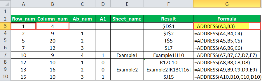
2. The Fifth Row
- The “row=5,” “column=20,” and “abs_num=2.”
- The ADDRESS formula can be rewritten in a simpler form as “=ADDRESS(5,20,2).”
- The reference style is set at 1 (true) when it has not been defined explicitly.
- The result is “T$5,” which has an absolute row ($5) and a relative column (T).
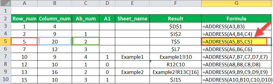
3. The Seventh Row
- We pass all the arguments of the ADDRESS function, including the optional ones.
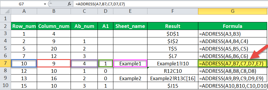
- The “row=10,” “column=9,” “abs_num=4,” “A1=1,” and “sheet_name=Example1.”
- The address formula can be rewritten in a simpler form as “=ADDRESS(10,9,4,1,”Example1″).”
- The result is “Example1!I10.”
- Since the “absolute number” parameter is set at 4, the result is a relative reference (“I10”).
How to Use the INDIRECT Function to Pass the Address?
The reference of a cell can be derived with the help of the ADDRESS function. However, if we are interested in obtaining the value stored in the Excel address of cells, we use the INDIRECT functionThe INDIRECT excel function is used to indirectly refer to cells, cell ranges, worksheets, and workbooks.read more. With this function, we can get the actual value through reference.
Syntax of the INDIRECT Function
The function accepts the following arguments:
- Ref_text: This is the cell reference supplied in the form of a text string.
- A1: This is a logical value that specifies the style of reference. It can be either “A1” (true or omitted) or “R1C1” (false).
The first argument is mandatory, while the second is optional.
Let us consider an example.
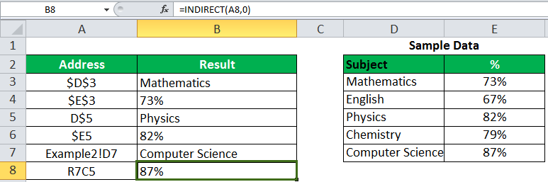
The data is given in the following image. We want to find the value of the cell reference passed in the INDIRECT function.
In the first observation, the “ADDRESS=$D$3.” We rewrite the function as “=INDIRECT(A3).”
In cell D3, under the sample data, the value is “Mathematics.” This is the same as the result of the INDIRECT function in cell B3.
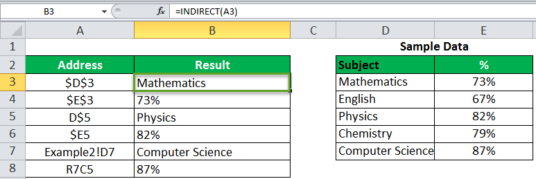
Let us consider another example in which the reference style is R7C5.
Here, we must set the “ref_type” to “false” (0), so that the INDIRECT function can read the reference style.
The output of “=INDIRECT(A8,0)” is 87%.
Frequently Asked Questions
What are the uses of the ADDRESS function of Excel?
The uses of the function are listed as follows:
– It is used to address the first or the last cell in a range.
– It helps convert a column number to a letter and vice versa.
– It is used to construct a cell reference within a formula.
– It helps find the cell value from the row and column number.
– It returns the address of the cell with the highest value.
How does the ADDRESS function return the address of the cell with the highest value?
The ADDRESS function is used in combination with the MATCH functionThe MATCH function looks for a specific value and returns its relative position in a given range of cells. The output is the first position found for the given value. Being a lookup and reference function, it works for both an exact and approximate match. For example, if the range A11:A15 consists of the numbers 2, 9, 8, 14, 32, the formula “MATCH(8,A11:A15,0)” returns 3. This is because the number 8 is at the third position.
read more to return the cell address with the highest value. The formula is stated as follows:
“=ADDRESS(MATCH(MAX(B:B),B:B,0),COLUMN(B2))”
The MAX functionThe MAX Formula in Excel is used to calculate the maximum value from a set of data/array. It counts numbers but ignores empty cells, text, the logical values TRUE and FALSE, and text values.read more returns the maximum value from the range “B:B.” The MATCH function looks for that maximum value and returns the row number (index). The column returns the column number of “B2.”
How does the ADDRESS function return the complete address of a named range?
The formula to return the full address of a named range is stated as follows:
“=ADDRESS(ROW(range), COLUMN(range)) & “:” & ADDRESS(ROW(range) + ROWS(range)-1, COLUMN(range) + COLUMNS(range)-1)”
“Range” is the named range whose address is required.
If the range address is required as a relative reference, the “abs_num” argument is set at 4. The formula can be rewritten as follows:
“=ADDRESS(ROW(range), COLUMN(range), 4) & “:” & ADDRESS(ROW(range) + ROWS(range)-1, COLUMN(range) + COLUMNS(range)-1, 4)”
- The ADDRESS function creates a cell address from a given row and column number.
- The syntax of the ADDRESS function is–“ADDRESS(row_num, column_num, [abs_num], [a1], [sheet_text]).”
- The “row_num” and “column_num” are mandatory arguments, while “abs_num,” “A1,” and “sheet_text” are optional arguments.
- The “abs_num” parameter can be set as follows:
- 1 or omitted–Absolute reference
- 2–Absolute row, relative column
- 3–Relative row, absolute column
- 4–Relative reference
- The reference style can be set at either “A1” (1 or true) or “R1C1” (0 or false).
- The default reference style is “A1.”
- The INDIRECT function helps obtain the value stored in the Excel address of cells. The syntax of the INDIRECT function is–“INDIRECT(ref_text, [a1]).”
Recommended Articles
This has been a guide to Address Excel Function. Here we discuss how to use the Address Formula in Excel along with step by step examples and downloadable Excel templates.`
- Excel Convert FunctionAs the word itself, the Excel CONVERT function defines that it can convert the numbers from one measurement system to another measurement system.read more
- Excel VBA MonthVBA Month Function is an inbuilt function that is used to extract the month from a date. The output of this function is an integer ranging from 1 to 12. Only the month number is extracted from the supplied date value by this function.read more
- PMT Excel Function
- Page Setup in ExcelTo set up a page in MS excel, in the page layout tab, click on the small arrow mark under the page setup group> A dialogue box will open, click on «fit to 1 page» option>go to print preview option and choose landscape mode>save changes, it’s done.
read more