Value not available excel

Этот урок объясняет, как быстро справиться с ситуацией, когда функция ВПР (VLOOKUP) не хочет работать в Excel 2013, 2010, 2007 и 2003, а также, как выявить и исправить распространённые ошибки и преодолеть ограничения ВПР.

В нескольких предыдущих статьях мы изучили различные грани функции ВПР в Excel. Если Вы читали их внимательно, то сейчас должны быть экспертом в этой области. Однако не без причины многие специалисты по Excel считают ВПР одной из наиболее сложных функций. Она имеет кучу ограничений и особенностей, которые становятся источником многих проблем и ошибок.

В этой статье Вы найдёте простые объяснения ошибок #N/A (#Н/Д), #NAME? (#ИМЯ?) и #VALUE! (#ЗНАЧ!), появляющихся при работе с функцией ВПР, а также приёмы и способы борьбы с ними. Мы начнём с наиболее частых случаев и наиболее очевидных причин, почему ВПР не работает, поэтому лучше изучать примеры в том порядке, в каком они приведены в статье.

• Исправляем ошибку #Н/Д
• Исправляем ошибку #ЗНАЧ! в формулах с ВПР
• Ошибка #ИМЯ? в ВПР
• ВПР не работает (проблемы, ограничения и решения)
• ВПР – работа с функциями ЕСЛИОШИБКА и ЕОШИБКА

Исправляем ошибку #Н/Д функции ВПР в Excel

В формулах с ВПР сообщение об ошибке #N/A (#Н/Д) – означает not available (нет данных) – появляется, когда Excel не может найти искомое значение. Это может произойти по нескольким причинам.

1. Искомое значение написано с опечаткой

Хорошая мысль проверить этот пункт в первую очередь! Опечатки часто возникают, когда Вы работаете с очень большими объёмами данных, состоящих из тысяч строк, или когда искомое значение вписано в формулу.

2. Ошибка #Н/Д при поиске приближённого совпадения с ВПР

Если Вы используете формулу с условием поиска приближённого совпадения, т.е. аргумент range_lookup (интервальный_просмотр) равен TRUE (ИСТИНА) или не указан, Ваша формула может сообщить об ошибке #Н/Д в двух случаях:

• Искомое значение меньше наименьшего значения в просматриваемом массиве.
• Столбец поиска не упорядочен по возрастанию.

3. Ошибка #Н/Д при поиске точного совпадения с ВПР

Если Вы ищете точное совпадение, т.е. аргумент range_lookup (интервальный_просмотр) равен FALSE (ЛОЖЬ) и точное значение не найдено, формула также сообщит об ошибке #Н/Д. Более подробно о том, как искать точное и приближенное совпадение с функцией ВПР.

4. Столбец поиска не является крайним левым

Как Вы, вероятно, знаете, одно из самых значительных ограничений ВПР это то, что она не может смотреть влево, следовательно, столбец поиска в Вашей таблице должен быть крайним левым. На практике мы часто забываем об этом, что приводит к не работающей формуле и появлению ошибки #Н/Д.

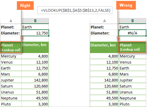
Решение: Если нет возможности изменить структуру данных так, чтобы столбец поиска был крайним левым, Вы можете использовать комбинацию функций ИНДЕКС (INDEX) и ПОИСКПОЗ (MATCH), как более гибкую альтернативу для ВПР.

5. Числа форматированы как текст

Другой источник ошибки #Н/Д в формулах с ВПР – это числа в текстовом формате в основной таблице или в таблице поиска.

Это обычно случается, когда Вы импортируете информацию из внешних баз данных или когда ввели апостроф перед числом, чтобы сохранить стоящий в начале ноль.

Наиболее очевидные признаки числа в текстовом формате показаны на рисунке ниже:

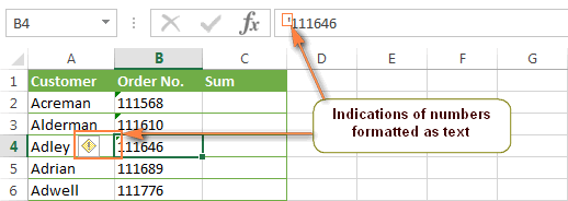
Кроме этого, числа могут быть сохранены в формате General (Общий). В таком случае есть только один заметный признак – числа выровнены по левому краю ячейки, в то время как стандартно они выравниваются по правому краю.

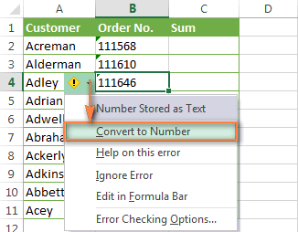
Решение: Если это одиночное значение, просто кликните по иконке ошибки и выберите Convert to Number (Конвертировать в число) из контекстного меню.

Если такая ситуация со многими числами, выделите их и щелкните по выделенной области правой кнопкой мыши. В появившемся контекстном меню выберите Format Cells (Формат ячеек) > вкладка Number (Число) > формат Number (Числовой) и нажмите ОК.

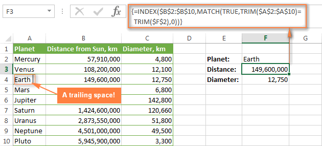
6. В начале или в конце стоит пробел

Это наименее очевидная причина ошибки #Н/Д в работе функции ВПР, поскольку зрительно трудно увидеть эти лишние пробелы, особенно при работе с большими таблицами, когда большая часть данных находится за пределами экрана.

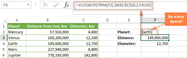
Решение 1: Лишние пробелы в основной таблице (там, где функция ВПР)

Если лишние пробелы оказались в основной таблице, Вы можете обеспечить правильную работу формул, заключив аргумент lookup_value (искомое_значение) в функцию TRIM (СЖПРОБЕЛЫ):

=VLOOKUP(TRIM($F2),$A$2:$C$10,3,FALSE)
=ВПР(СЖПРОБЕЛЫ($F2);$A$2:$C$10;3;ЛОЖЬ)

Решение 2: Лишние пробелы в таблице поиска (в столбце поиска)

Если лишние пробелы оказались в столбце поиска – простыми путями ошибку #Н/Д в формуле с ВПР не избежать. Вместо ВПР Вы можете использовать формулу массива с комбинацией функций ИНДЕКС (INDEX), ПОИСКПОЗ (MATCH) и СЖПРОБЕЛЫ (TRIM):

=INDEX($C$2:$C$10,MATCH(TRUE,TRIM($A$2:$A$10)=TRIM($F$2),0))
=ИНДЕКС($C$2:$C$10;ПОИСКПОЗ(ИСТИНА;СЖПРОБЕЛЫ($A$2:$A$10)=СЖПРОБЕЛЫ($F$2);0))

Так как это формула массива, не забудьте нажать Ctrl+Shift+Enter вместо привычного Enter, чтобы правильно ввести формулу.

Ошибка #ЗНАЧ! в формулах с ВПР

В большинстве случаев, Microsoft Excel сообщает об ошибке #VALUE! (#ЗНАЧ!), когда значение, использованное в формуле, не подходит по типу данных. Что касается ВПР, то обычно выделяют две причины ошибки #ЗНАЧ!.

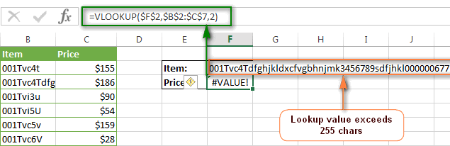
1. Искомое значение длиннее 255 символов

Будьте внимательны: функция ВПР не может искать значения, содержащие более 255 символов. Если искомое значение превышает этот предел, то Вы получите сообщение об ошибке #ЗНАЧ!.

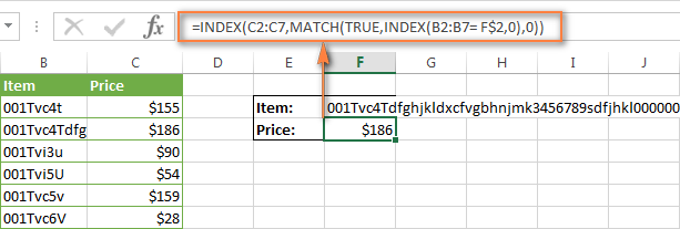
Решение: Используйте связку функций ИНДЕКС+ПОИСКПОЗ (INDEX+MATCH). Ниже представлена формула, которая отлично справится с этой задачей:

=INDEX(C2:C7,MATCH(TRUE,INDEX(B2:B7=F$2,0),0))
=ИНДЕКС(C2:C7;ПОИСКПОЗ(ИСТИНА;ИНДЕКС(B2:B7=F$2;0);0))

2. Не указан полный путь к рабочей книге для поиска

Если Вы извлекаете данные из другой рабочей книги, то должны указать полный путь к этому файлу. Если говорить точнее, Вы должны указать имя рабочей книги (включая расширение) в квадратных скобках [ ], далее указать имя листа, а затем – восклицательный знак. Всю эту конструкцию нужно заключить в апострофы, на случай если имя книги или листа содержит пробелы.

Вот полная структура функции ВПР для поиска в другой книге:

=VLOOKUP(lookup_value,'[workbook name]sheet name'!table_array, col_index_num,FALSE)
=ВПР(искомое_значение;'[имя_книги]имя_листа'!таблица;номер_столбца;ЛОЖЬ)

Настоящая формула может выглядеть так:

=VLOOKUP($A$2,'[New Prices.xls]Sheet1'!$B:$D,3,FALSE)
=ВПР($A$2;'[New Prices.xls]Sheet1'!$B:$D;3;ЛОЖЬ)

Эта формула будет искать значение ячейки A2 в столбце B на листе Sheet1 в рабочей книге New Prices и извлекать соответствующее значение из столбца D.

Если любая часть пути к таблице пропущена, Ваша функция ВПР не будет работать и сообщит об ошибке #ЗНАЧ! (даже если рабочая книга с таблицей поиска в данный момент открыта).

Для получения дополнительной информации о функции ВПР, ссылающейся на другой файл Excel, обратитесь к уроку: Поиск в другой рабочей книге с помощью ВПР.

3. Аргумент Номер_столбца меньше 1

Трудно представить ситуацию, когда кто-то вводит значение меньше 1, чтобы обозначить столбец, из которого нужно извлечь значение. Хотя это возможно, если значение этого аргумента вычисляется другой функцией Excel, вложенной в ВПР.

Итак, если случилось, что аргумент col_index_num (номер_столбца) меньше 1, функция ВПР также сообщит об ошибке #ЗНАЧ!.

Если же аргумент col_index_num (номер_столбца) больше количества столбцов в заданном массиве, ВПР сообщит об ошибке #REF! (#ССЫЛ!).

Ошибка #ИМЯ? в ВПР

Простейший случай – ошибка #NAME? (#ИМЯ?) – появится, если Вы случайно напишите с ошибкой имя функции.

Решение очевидно – проверьте правописание!

ВПР не работает (ограничения, оговорки и решения)

Помимо достаточно сложного синтаксиса, ВПР имеет больше ограничений, чем любая другая функция Excel. Из-за этих ограничений, простые на первый взгляд формулы с ВПР часто приводят к неожиданным результатам. Ниже Вы найдёте решения для нескольких распространённых сценариев, когда ВПР ошибается.

1. ВПР не чувствительна к регистру

Функция ВПР не различает регистр и принимает символы нижнего и ВЕРХНЕГО регистра как одинаковые. Поэтому, если в таблице есть несколько элементов, которые различаются только регистром символов, функция ВПР возвратит первый попавшийся элемент, не взирая на регистр.

Решение: Используйте другую функцию Excel, которая может выполнить вертикальный поиск (ПРОСМОТР, СУММПРОИЗВ, ИНДЕКС и ПОИСКПОЗ) в сочетании с СОВПАД, которая различает регистр. Более подробно Вы можете узнать из урока — 4 способа сделать ВПР с учетом регистра в Excel.

2. ВПР возвращает первое найденное значение

Как Вы уже знаете, ВПР возвращает из заданного столбца значение, соответствующее первому найденному совпадению с искомым. Однако, Вы можете заставить ее извлечь 2-е, 3-е, 4-е или любое другое повторение значения, которое Вам нужно. Если нужно извлечь все повторяющиеся значения, Вам потребуется комбинация из функций ИНДЕКС (INDEX), НАИМЕНЬШИЙ (SMALL) и СТРОКА (ROW).

3. В таблицу был добавлен или удалён столбец

К сожалению, формулы с ВПР перестают работать каждый раз, когда в таблицу поиска добавляется или удаляется новый столбец. Это происходит, потому что синтаксис ВПР требует указывать полностью весь диапазон поиска и конкретный номер столбца для извлечения данных. Естественно, и заданный диапазон, и номер столбца меняются, когда Вы удаляете столбец или вставляете новый.

Решение: И снова на помощь спешат функции ИНДЕКС (INDEX) и ПОИСКПОЗ (MATCH). В формуле ИНДЕКС+ПОИСКПОЗ Вы раздельно задаёте столбцы для поиска и для извлечения данных, и в результате можете удалять или вставлять сколько угодно столбцов, не беспокоясь о том, что придётся обновлять все связанные формулы поиска.

4. Ссылки на ячейки исказились при копировании формулы

Этот заголовок исчерпывающе объясняет суть проблемы, правда?

Решение: Всегда используйте абсолютные ссылки на ячейки (с символом $) при записи диапазона, например $A$2:$C$100 или $A:$C. В строке формул Вы можете быстро переключать тип ссылки, нажимая F4.

ВПР – работа с функциями ЕСЛИОШИБКА и ЕОШИБКА

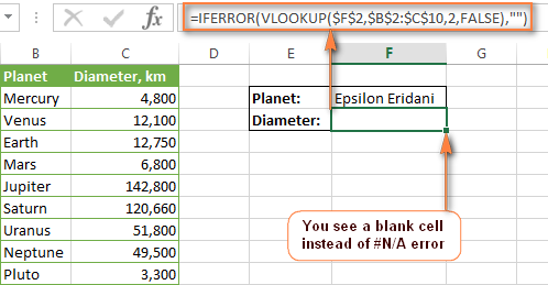
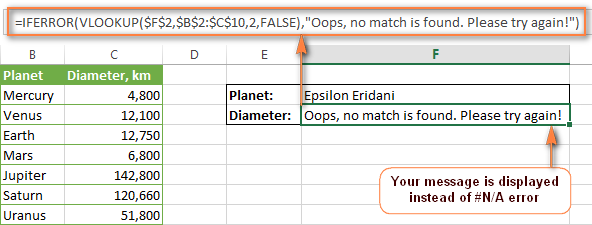
Если Вы не хотите пугать пользователей сообщениями об ошибках #Н/Д, #ЗНАЧ! или #ИМЯ?, можете показывать пустую ячейку или собственное сообщение. Вы можете сделать это, поместив ВПР в функцию ЕСЛИОШИБКА (IFERROR) в Excel 2013, 2010 и 2007 или использовать связку функций ЕСЛИ+ЕОШИБКА (IF+ISERROR) в более ранних версиях.

ВПР: работа с функцией ЕСЛИОШИБКА

Синтаксис функции ЕСЛИОШИБКА (IFERROR) прост и говорит сам за себя:

IFERROR(value,value_if_error)
ЕСЛИОШИБКА(значение;значение_если_ошибка)

То есть, для первого аргумента Вы вставляете значение, которое нужно проверить на предмет ошибки, а для второго аргумента указываете, что нужно возвратить, если ошибка найдётся.

Например, вот такая формула возвращает пустую ячейку, если искомое значение не найдено:

=IFERROR(VLOOKUP($F$2,$B$2:$C$10,2,FALSE),"")
=ЕСЛИОШИБКА(ВПР($F$2;$B$2:$C$10;2;ЛОЖЬ);"")

Если Вы хотите показать собственное сообщение вместо стандартного сообщения об ошибке функции ВПР, впишите его в кавычках, например, так:

=IFERROR(VLOOKUP($F$2,$B$2:$C$10,2,FALSE),"Ничего не найдено. Попробуйте еще раз!")
=ЕСЛИОШИБКА(ВПР($F$2;$B$2:$C$10;2;ЛОЖЬ);"Ничего не найдено. Попробуйте еще раз!")

ВПР: работа с функцией ЕОШИБКА

Так как функция ЕСЛИОШИБКА появилась в Excel 2007, при работе в более ранних версиях Вам придётся использовать комбинацию ЕСЛИ (IF) и ЕОШИБКА (ISERROR) вот так:

=IF(ISERROR(VLOOKUP формула),"Ваше сообщение при ошибке",VLOOKUP формула)
=ЕСЛИ(ЕОШИБКА(ВПР формула);"Ваше сообщение при ошибке";ВПР формула)

Например, формула ЕСЛИ+ЕОШИБКА+ВПР, аналогична формуле ЕСЛИОШИБКА+ВПР, показанной выше:

=IF(ISERROR(VLOOKUP($F$2,$B$2:$C$10,2,FALSE)),"",VLOOKUP($F$2,$B$2:$C$10,2,FALSE))
=ЕСЛИ(ЕОШИБКА(ВПР($F$2;$B$2:$C$10;2;ЛОЖЬ));"";ВПР($F$2;$B$2:$C$10;2;ЛОЖЬ))

На сегодня всё. Надеюсь, этот короткий учебник поможет Вам справиться со всеми возможными ошибками ВПР и заставит Ваши формулы работать правильно.

I recommend that you look into the combination of INDEX & MATCH, rather than VLOOKUP, for situations like this. VLOOKUP has 2 main flaws: (1) you have to order your data so that your search term is the left-most column of a continuous data block [as you have just seen]; and (2) it is volatile, meaning that when a column is inserted within your data block, it will no longer properly ‘count’ the number of columns to move to retrieve your data.

MATCH is like half of VLOOKUP. You give MATCH a specific column or row, and a value to search for, and it will simply return the number of cells in it had to move to find that value.

=MATCH(A1,B:B,0)

This says ‘look at B:B, and tell me what row the value of A1 appears on’.

INDEX is like the other half of VLOOKUP. You give INDEX a group of cells (either a row, column, or a 2D range), and a specific row number (plus potentially a column number), and it will return the value for that cell.

=INDEX(C:C,5)

This gives you the value of cell C5, which is the 5th row found in the column given to INDEX. Combine these two formulas and it will return the value of column C, where column B matches A1:

=INDEX(C:C,MATCH(A1,B:B,0))

This formula gives an identical result to

=VLOOKUP(A1,B:C,0)

VLOOKUP looks simpler here, but INDEX & MATCH is much more versatile — in your case, you wouldn’t have needed to reorder your data to get it to work, you could have used the formula:

=INDEX('Raw Data'!I:I,MATCH(E9,'Raw Data'!E:E,0))

Once you get into the habit of using INDEX / MATCH over vlookup, you will find that your data is a lot more flexible to manage.

You may have encountered an error message that says the “Value not available” error is in vlookup. It turns out that there are several ways to solve this problem, which we will talk about a little later.

Updated

1. Download ASR Pro

2. Run the program

3. Click «Scan Now» to find and remove any viruses on your computer

Speed up your computer today with this simple download.

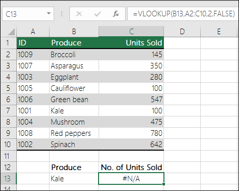
g.Often the only common cause of a #N / ​​A error is related to VLOOKUP, HLOOKUP, LOOKUP, or MATCH, where the formula cannot find a suitable reference value. For example, your search weight does not exist in the original data. In this case, “banana” is not mentioned in the lookup table, so the positive aspects of VLOOKUP are the # N / A error.

g.Stands

vlookup is called “vertical search” and its osThe new feature is that you can search for values ​​in one column (vertically) and then return the matching value from multiple cells in a row of that value (horizontally). For example, if you find yourself at a restaurant counter, search the list of products and then just look at the price once you find an item that matches your order. Sometimes it can be tricky to use the basic syntax for VLOOKUP. In this case, a terrible # n / a result may be returned, although you can look directly at the market value in the column.

What Does “# N / A” Actually Mean For An Exact Result?

# N / A is short for “not available”, which means that the scan cannot return a value or only found a match. This result can be returned even if there are matches in the column, if the VLOOKUP syntax is clearly poorly constructed. Some of your problems may lead to # N / A being fired.

Common Causes Of # N / A In VLOOKUP

Most of the time it returns # N / A because the actual data in the table cell is definitely not the same as They appear in the table. There are several possible reasons for the discrepancy between the way statistics are stored and what is displayed in a table cell.

1. Numbers Are Formatted With Text

If a table cell is formatted exactly like text, it will be treated as a type even if it contains numbers, dates, and other data that is not normally handled in the same way as plain text. If you are looking for explicit numbers and cells are formatted as copies, # N / A may be returned because an exact match cannot be found due to different data types. The most common way to prevent this is to select the desired table cells so that they can be found, and then right-click them to format them with the appropriate data type on your computer’s hard drive.

Because column B is formatted as text, the search dollar value must be enclosed in double quotes, otherwise the column must often be reformatted to a numeric data type.

2. Add Much More To Table Lookup Values ​​

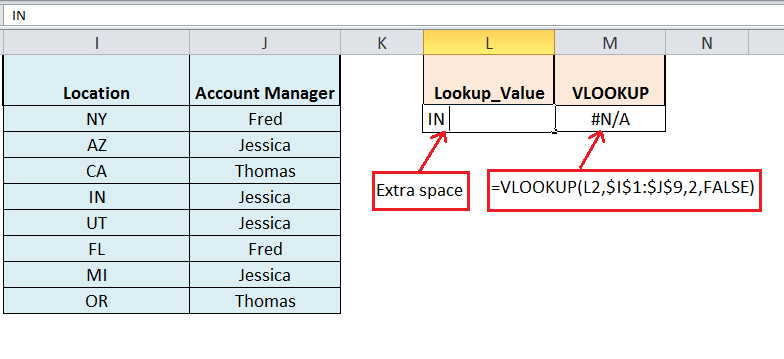
Ca Any stylistic problem in spreadsheets or just data in Commander is leading or trailing spaces in a particular data item. Because the VLOOKUP function searches for a strict exact match, it will not find a new matching cell if the data contains spaces at the beginning or end of a specified value. To resolve this issue, make sure buildings are removed from the column cells. This can be achieved by using the CROP function in addition to the FIND AND REPLACE method, or by using an Excel add-in to clear cells.

The value relative to cell B2 “2019” does indeed contain a space that caused this # N / A error.

3. Error In Lookup_value Syntax, Battle Of VLOOKUP

You might think that this particular case would be uncomplicated, only it is very easy to make typos and other useful errors in the lookup_value parameter when designing the syntax for a VLOOKUP formula. Make sure you type and enter the search term correctly, that the program is entered in the correct upper and lower case letters and does not contain leading or trailing spaces.

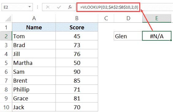
4. The Search Value Is Not Far To The Left In The Array е Array

Make sure the perks you want are in the leftmost column, which is in the furniture array of the second parameter of some VLOOKUP formula. Typos in the cellset will invalidate the search. Handle this setting with care. Also, if the command does contain a value, but it is the wrong column, your formula will return the wrong values ​​to your desktop.

Sometimes the result is returned # N / A just because the syntax of the VLOOKUP formula is incorrect. An example would be an incorrect search for a value in a parameter list. Make sure the value you are looking for is in the leftmost parameter or the first parameter in the formula. Example: VLOOKUP (lookup_value, table_array, col_index_num, [range_lookup]).

These are just 4 of the most common Excel VLOOKUP errors that lead to the dreaded # N / A error message. Excel is extremely powerful and has many features. The best way to become an Excel expert and learn how to use all this data magic is with Excel training.

Why not start your journey and your free time to becomeAre you a certified Excel master today?

Speed up your computer today with this simple download.

검색 문제에서 “값을 사용할 수 없음” 오류를 수정하는 가장 좋은 방법 V
Najlepszy Sposób Na Naprawienie Błędu „wartość Niedostępna” W Problemach Z Wyszukiwaniem V
Bästa Sättet Att Fixa Felet “värde Ej Tillgängligt” I Sökproblem V
Il Modo Migliore Per Correggere L’errore “valore Non Disponibile” Nei Problemi Di Ricerca V
Meilleur Moyen De Corriger L’erreur “valeur Non Disponible” Dans Les Problèmes De Recherche V
Melhor Maneira De Corrigir O Erro “valor Não Disponível” Em Problemas De Pesquisa V
Beste Möglichkeit, Den Fehler „Wert Nicht Verfügbar“ Bei Suchproblemen Zu Beheben V
Лучший способ исправить ошибку «значение недоступно» в проблемах поиска V
De Beste Manier Om De “waarde Niet Beschikbaar”-fout In Zoekproblemen Op Te Lossen V
La Mejor Manera De Corregir El Error “valor No Disponible” En Los Problemas De Búsqueda V

1. 04-14-2005, 12:06 PM

   
   

   #1

   Value Not Available Error in Vlookup
   

   I’m using the vlookup function to get a number back from a table. I’ve
   created the vlookup properly but keep getting the #N/A with the message —
   «Value Not Available Error». The problem is that the value is available.
   I’ve copied the vlookup formula into a number of cells — all come back #N/A.
   The puzzle is, I can get the formula to work if I retype the value being
   looked up in the table. I’ve compared formats; I’ve made sure the table is
   in alphabetical order; I can’t see any difference from the value being looked
   up with the value in the table — they are even the same font.
   Any ideas? The table is copied into the worksheet from another workbook.
   Thanks for any help.

   ---

2. 04-14-2005, 01:06 PM

   
   

   #2

   Re: Value Not Available Error in Vlookup
   

   Hi

   when you retype the value being lookup it tends to suggest a problem along
   the lines of:
   — calculation set to manual — tools / options / calculation -check that it
   is set to automatic
   — leading or trailing spaces in this value in the lookup value — type in
   another cell =LEN(A1) where A1 is the cell reference of your lookup value to
   find out how many characters excel sees the cell as having as compared to
   how many you think it has
   — numbers that aren’t really numbers if you’re looking up numbers — type in
   another cell =ISNUMBER(A1) to test that what you think is a number is
   acutally a number
   -omitting the 4th parameter (0 or FALSE) for an exact match — although this
   would normally raise wrong answers rather than an #NA error

   hope this helps
   —
   Cheers
   JulieD
   check out www.hcts.net.au/tipsandtricks.htm
   ….well i’m working on it anyway
   «thefeokas» <thefeokas@discussions.microsoft.com> wrote in message
   news:65416377-E39F-4150-A189-DBDCEA3F49CF@microsoft.com…

   
   > I’m using the vlookup function to get a number back from a table. I’ve
   > created the vlookup properly but keep getting the #N/A with the message —
   > «Value Not Available Error». The problem is that the value is available.
   > I’ve copied the vlookup formula into a number of cells — all come back
   > #N/A.
   > The puzzle is, I can get the formula to work if I retype the value being
   > looked up in the table. I’ve compared formats; I’ve made sure the table
   > is
   > in alphabetical order; I can’t see any difference from the value being
   > looked
   > up with the value in the table — they are even the same font.
   > Any ideas? The table is copied into the worksheet from another workbook.
   > Thanks for any help.

   ---

3. 04-14-2005, 01:06 PM

   
   

   #3

   Re: Value Not Available Error in Vlookup
   

   That did it! I found that there were spaces in the lookup table at the end of
   the values. I used Replace… to remove the trailing spaces.
   Thanks.

   «JulieD» wrote:

   
   > Hi
   >
   > when you retype the value being lookup it tends to suggest a problem along
   > the lines of:
   > — calculation set to manual — tools / options / calculation -check that it
   > is set to automatic
   > — leading or trailing spaces in this value in the lookup value — type in
   > another cell =LEN(A1) where A1 is the cell reference of your lookup value to
   > find out how many characters excel sees the cell as having as compared to
   > how many you think it has
   > — numbers that aren’t really numbers if you’re looking up numbers — type in
   > another cell =ISNUMBER(A1) to test that what you think is a number is
   > acutally a number
   > -omitting the 4th parameter (0 or FALSE) for an exact match — although this
   > would normally raise wrong answers rather than an #NA error
   >
   > hope this helps
   > —
   > Cheers
   > JulieD
   > check out www.hcts.net.au/tipsandtricks.htm
   > ….well i’m working on it anyway
   > «thefeokas» <thefeokas@discussions.microsoft.com> wrote in message
   > news:65416377-E39F-4150-A189-DBDCEA3F49CF@microsoft.com…
   > > I’m using the vlookup function to get a number back from a table. I’ve
   > > created the vlookup properly but keep getting the #N/A with the message —
   > > «Value Not Available Error». The problem is that the value is available.
   > > I’ve copied the vlookup formula into a number of cells — all come back
   > > #N/A.
   > > The puzzle is, I can get the formula to work if I retype the value being
   > > looked up in the table. I’ve compared formats; I’ve made sure the table
   > > is
   > > in alphabetical order; I can’t see any difference from the value being
   > > looked
   > > up with the value in the table — they are even the same font.
   > > Any ideas? The table is copied into the worksheet from another workbook.
   > > Thanks for any help.
   >
   >
   >

   ---

4. 04-14-2005, 01:06 PM

   
   

   #4

   Re: Value Not Available Error in Vlookup
   

   you’re welcome and thanks for the feedback

   —
   Cheers
   JulieD
   check out www.hcts.net.au/tipsandtricks.htm
   ….well i’m working on it anyway
   «thefeokas» <thefeokas@discussions.microsoft.com> wrote in message
   news:62E30085-F56C-42F5-8C8C-D1DAABED6CF2@microsoft.com…

   
   > That did it! I found that there were spaces in the lookup table at the end
   > of
   > the values. I used Replace… to remove the trailing spaces.
   > Thanks.
   >
   > «JulieD» wrote:
   >
   >> Hi
   >>
   >> when you retype the value being lookup it tends to suggest a problem
   >> along
   >> the lines of:
   >> — calculation set to manual — tools / options / calculation -check that
   >> it
   >> is set to automatic
   >> — leading or trailing spaces in this value in the lookup value — type in
   >> another cell =LEN(A1) where A1 is the cell reference of your lookup value
   >> to
   >> find out how many characters excel sees the cell as having as compared to
   >> how many you think it has
   >> — numbers that aren’t really numbers if you’re looking up numbers — type
   >> in
   >> another cell =ISNUMBER(A1) to test that what you think is a number is
   >> acutally a number
   >> -omitting the 4th parameter (0 or FALSE) for an exact match — although
   >> this
   >> would normally raise wrong answers rather than an #NA error
   >>
   >> hope this helps
   >> —
   >> Cheers
   >> JulieD
   >> check out www.hcts.net.au/tipsandtricks.htm
   >> ….well i’m working on it anyway
   >> «thefeokas» <thefeokas@discussions.microsoft.com> wrote in message
   >> news:65416377-E39F-4150-A189-DBDCEA3F49CF@microsoft.com…
   >> > I’m using the vlookup function to get a number back from a table. I’ve
   >> > created the vlookup properly but keep getting the #N/A with the
   >> > message —
   >> > «Value Not Available Error». The problem is that the value is
   >> > available.
   >> > I’ve copied the vlookup formula into a number of cells — all come back
   >> > #N/A.
   >> > The puzzle is, I can get the formula to work if I retype the value
   >> > being
   >> > looked up in the table. I’ve compared formats; I’ve made sure the
   >> > table
   >> > is
   >> > in alphabetical order; I can’t see any difference from the value being
   >> > looked
   >> > up with the value in the table — they are even the same font.
   >> > Any ideas? The table is copied into the worksheet from another
   >> > workbook.
   >> > Thanks for any help.
   >>
   >>
   >>

   ---

PC running slow?

1. Download ASR Pro from the website

2. Install it on your computer

3. Run the scan to find any malware or virus that might be lurking in your system

Improve the speed of your computer today by downloading this software — it will fix your PC problems.

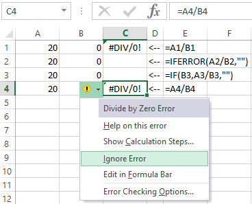
If you know how to remove the “Value is not available” error in Excel on your computer, this blog post will help you solve it. g.To fix the error, we can use someone else’s IFERROR () function that was introduced in Excel 2007. We use our original vlookup function as the first argument. Next, we form a comma and specify what should appear when the vlookup function returns an error.

g.

Excel for Microsoft 365 Excel 2021 Excel 2019 Excel 2016 Excel 2013 Excel 2010 Excel 2007 Aria-label = “Press Enter More … Less

Excel for Microsoft 365 Excel 2021 Excel 2019 Excel 2016 Excel 2013 Excel 2010 Excel 2007 More ….. Less

Use the following procedure to format misspelled cells so that text on these phones appears in white. As a result, the error text is sold practically invisible in this fabric.

1. The selected range of

   cells containing each of our error values.

2. On the Home tab, in the Styles group, click the arrow next to Conditional Formatting and select Manage Rules.
   The Conditional Rule Formatting Manager dialog box appears.

3. Click New Rule.
   Displays the “New Formatting Dialog” rule field.

4. Under Select a Functional Rule Type, click Format Only Cells Containing Ideas.

5. Under Edit Rule Description, under Format only cells with, select Error.

6. Click Format, then click the Font tab.

7. Click the arrowup to open a list of colors, and select white under Theme Colors.

There are times when you don’t want to display error values ​​in cells and prefer to display text instead, such as the string for “# N / A”, a hyphen, or the string “NA”. To do this, you can use the IFEROR and NA functions, as shown in the following example.

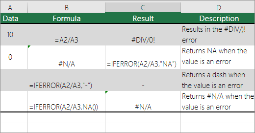
Function details

IFERROR Use this intent to determine if a cell contains a valid error or if formula results return an error.

NA Use this function to return wire # N / A to the cell. The syntax is considered = NA ().

1. Click on one of our pivot table reports.
   The PivotTable Tools will appear.

2. PC running slow?

   ASR Pro is the ultimate solution for your PC repair needs! Not only does it swiftly and safely diagnose and repair various Windows issues, but it also increases system performance, optimizes memory, improves security and fine tunes your PC for maximum reliability. So why wait? Get started today!

   

   Excel 2016 and Excel 2013: Under Variance Analysis, in the PivotTable group, click the pointer next to the Options box and select Options.

   Excel 2010 and Excel 2007: On the Options tab, in the PivotTable cluster, click the arrow next to the Options box and select Options.

3. Click Disposition and Format Loss, then do one or more of the following:

   • Change the display of errors. Under Format, select Validate Package to display the error values. In the field, you can display the value of the type for which you want to display errors. To display errors as blank cells, remove all characters in most fields.

   • Change the display of empty cells. Select the Show Blank Cells check box. In the box, enter the value you want to display in the available cells. To display blank cells, remove characters from the field. To display pure zeros, select the checkbox.

If a cell contains a formula that results in an error, a circle will appear in the upper left basket of the cell (error indicator). You can prevent these views from appearing using the following procedures.

1. In Excel 2016, Excel 2013, and Excel 2010: Click File> Options> Formulas.

   In Excel 2007: Click the Microsoft Office button > Excel Options> Formulas.

2. Under Error Checking, clear the Enable Error Checking for Queries check box.

Improve the speed of your computer today by downloading this software — it will fix your PC problems.

So Verschieben Sie Den Fehler “Wert Nicht Verfügbar” In Excel Easy-Lösung
Comment Supprimer L’erreur “Valeur Non Disponible” Dans La Solution Excel Easy
Как устранить ошибку “Значение недоступно” в решении Excel Easy
Hoe De “Waarde Gewoon Niet Beschikbaar”-fout In Excel Easy-oplossing Te Verwijderen
Jak Faktycznie Usunąć Błąd „Wartość Niedostępna” W Rozwiązaniu Excel Easy
Cómo Eliminar El Error “Valor No Disponible” En Excel Easy Solution
Come Rimuovere L’errore “Valore Non Più Disponibile” Nella Soluzione Excel Easy
Excel Easy 솔루션에서 “값을 사용할 수 없음” 오류를 제거하는 방법
Como Evitar O Erro “Valor Não Disponível” Na Solução Fácil Do Excel
Hur Man Tar Bort “Value N’t Available” -fel I Excel Easy -lösning