
Excel for Microsoft 365 Excel 2021 Excel 2019 Excel 2016 Excel 2013 Excel 2010 Excel 2007 More…Less
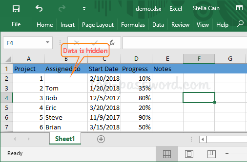
Suppose you have a worksheet that contains confidential information, such as employee salaries, that you do not want a co-worker who stops by your desk to see. Or perhaps you multiply the values in a range of cells by the value in another cell that you do not want to be visible on the worksheet. By applying a custom number format, you can hide the values of those cells on the worksheet.
Note: Although cells with hidden values appear blank on the worksheet, their values remain displayed in the formula bar where you can work with them.
Hide cell values
-
Select the cell or range of cells that contains values that you want to hide. For more information, see Select cells, ranges, rows, or columns on a worksheet .
Note: The selected cells will appear blank on the worksheet, but a value appears in the formula bar when you click one of the cells.
-
On the Home tab, click the Dialog Box Launcher
 next to Number.
-
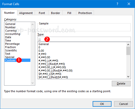
In the Category box, click Custom.
-
In the Type box, select the existing codes.
-
Type ;;; (three semicolons).
-
Click OK.
Tip: To cancel a selection of cells, click any cell on the worksheet.
Display hidden cell values
-
Select the cell or range of cells that contains values that are hidden. For more information, see Select cells, ranges, rows, or columns on a worksheet .
-
On the Home tab, click the Dialog Box Launcher
next to Number.
-
In the Category box, click General to apply the default number format, or click the date, time, or number format that you want.
Tip: To cancel a selection of cells, click any cell on the worksheet.
Need more help?
Want more options?
Explore subscription benefits, browse training courses, learn how to secure your device, and more.
Communities help you ask and answer questions, give feedback, and hear from experts with rich knowledge.
Excel for Microsoft 365 for Mac Excel 2021 for Mac Excel 2019 for Mac Excel 2016 for Mac Excel for Mac 2011 More…Less
If you have a sheet that contains confidential information, such as employee salaries, you can hide the values of those cells by using a custom number format.
Do any of the following:
Hide cell values
When you hide a value in a cell, the cell appears to be empty. However, the formula bar still contains the value.
-
Select the cells.
-
On the Format menu, click Cells, and then click the Number tab.
-
Under Category, click Custom.
-
In the Type box, type ;;; (that is, three semicolons in a row), and then click OK.
Display hidden cell values
-
Select the cells.
-
On the Format menu, click Cells, and then click the Number tab.
-
Under Category, click General (or any appropriate date, time, or number format other than Custom), and then click OK.
See also
Protect workbooks or sheets (2016)
Protect a workbook
Protect a sheet (2011)
Need more help?
Conditional formatting of Excel cells simplifies
highlighting values by adding color scales,
data bars, sparklines, and in-cell icons to the cell. The exact values of the highlighted cells
are rarely meaningful and may even interfere with the perception of information. Custom cell format
allows hiding values of such cells without hiding the cells.

1. Select cells which values you want to hide and do
one of the following:
- Right-click on the selection and choose Format Cells… in the popup menu:

- On the Home tab, in the Number group, click the dialog box launcher:


2. In the Format Cells dialog box, on the Number
tab, select the Custom formatting, and then in the Type field, type «;;;»
to hide any value in the cells:

Note: The format code has four sections separated by semicolons:
Positive; Negative; Zero; Text
The empty sections mean no visible content to show.
See
Custom cell format for more details.
Please, disable AdBlock and reload the page to continue
Today, 30% of our visitors use Ad-Block to block ads.We understand your pain with ads, but without ads, we won’t be able to provide you with free content soon. If you need our content for work or study, please support our efforts and disable AdBlock for our site. As you will see, we have a lot of helpful information to share.
Содержание
- Hide error values and error indicators in cells
- Convert an error to zero and use a format to hide the value
- Hide or display cell values
- Hide cell values
- Display hidden cell values
- How to Hide Rows based on Cell Value in Excel?
- Using Filters to Hide Rows based on Cell Value
- Using VBA to Hide Rows based on Cell Value
- Writing the VBA Code
- Running the Macro
- Explanation of the Code
- Un-hiding Columns Based On Cell Value
- Hiding Rows Based On Cell Values in Real-Time
- The Worksheet_SelectionChange Event
- Writing the VBA Code
- Running the Macro
- Explanation of the Code
Hide error values and error indicators in cells
Let’s say that your spreadsheet formulas have errors that you anticipate and don’t need to correct, but you want to improve the display of your results. There are several ways to hide error values and error indicators in cells.
There are many reasons why formulas can return errors. For example, division by 0 is not allowed, and if you enter the formula =1/0, Excel returns #DIV/0. Error values include #DIV/0!, #N/A, #NAME?, #NULL!, #NUM!, #REF!, and #VALUE!.
Convert an error to zero and use a format to hide the value
You can hide error values by converting them to a number such as 0, and then applying a conditional format that hides the value.
Create an example error
Open a blank workbook, or create a new worksheet.
Enter 3 in cell B1, enter 0 in cell C1, and in cell A1, enter the formula =B1/C1.
The #DIV/0! error appears in cell A1.
Select A1, and press F2 to edit the formula.
After the equal sign (=), type IFERROR followed by an opening parenthesis.
IFERROR(
Move the cursor to the end of the formula.
Type ,0 ) – that is, a comma followed by a zero and a closing parenthesis.
The formula =B1/C1 becomes =IFERROR(B1/C1 ,0).
Press Enter to complete the formula.
The contents of the cell should now display 0 instead of the #DIV! error.
Apply the conditional format
Select the cell that contains the error, and on the Home tab, click Conditional Formatting.
In the New Formatting Rule dialog box, click Format only cells that contain.
Under Format only cells with, make sure Cell Value appears in the first list box, equal to appears in the second list box, and then type 0 in the text box to the right.
Click the Format button.
Click the Number tab and then, under Category, click Custom.
In the Type box, enter ;;; (three semicolons), and then click OK. Click OK again.
The 0 in the cell disappears. This happens because the ;;; custom format causes any numbers in a cell to not be displayed. However, the actual value (0) remains in the cell.
Use the following procedure to format cells that contain errors so that the text in those cells is displayed in a white font. This makes the error text in these cells virtually invisible.
Select the range of cells that contain the error value.
On the Home tab, in the Styles group, click the arrow next to Conditional Formatting and then click Manage Rules.
The Conditional Formatting Rules Manager dialog box appears.
Click New Rule.
The New Formatting Rule dialog box appears.
Under Select a Rule Type, click Format only cells that contain.
Under Edit the Rule Description, in the Format only cells with list, select Errors.
Click Format, and then click the Font tab.
Click the arrow to open the Color list, and under Theme Colors, select the white color.
There may be times when you do not want error vales to appear in cells, and would prefer that a text string such as “#N/A,” a dash, or the string “NA” appears instead. To do this, you can use the IFERROR and NA functions, as the following example shows.
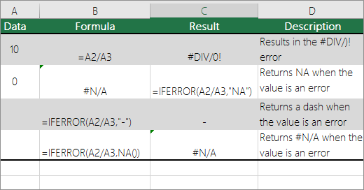
IFERROR Use this function to determine if a cell contains an error or if the results of a formula will return an error.
NA Use this function to return the string #N/A in a cell. The syntax is = NA().
Click the PivotTable report.
The PivotTable Tools appear.
Excel 2016 and Excel 2013: On the Analyze tab, in the PivotTable group, click the arrow next to Options, and then click Options.
Excel 2010 and Excel 2007: On the Options tab, in the PivotTable group, click the arrow next to Options, and then click Options.
Click the Layout & Format tab, and then do one or more of the following:
Change error display Select the For error values show check box under Format. In the box, type the value that you want to display instead of errors. To display errors as blank cells, delete any characters in the box.
Change empty cell display Select the For empty cells show check box. In the box, type the value that you want to display in empty cells. To display blank cells, delete any characters in the box. To display zeros, clear the check box.
If a cell contains a formula that results in an error, a triangle (an error indicator) appears in the top-left corner of the cell. You can prevent these indicators from being displayed by using the following procedure.

Cell with a formula problem
In Excel 2016, Excel 2013, and Excel 2010: Click File > Options > Formulas.
In Excel 2007: Click the Microsoft Office Button  > Excel Options > Formulas.
Under Error Checking, clear the Enable background error checking check box.
Источник
Hide or display cell values
Suppose you have a worksheet that contains confidential information, such as employee salaries, that you do not want a co-worker who stops by your desk to see. Or perhaps you multiply the values in a range of cells by the value in another cell that you do not want to be visible on the worksheet. By applying a custom number format, you can hide the values of those cells on the worksheet.
Note: Although cells with hidden values appear blank on the worksheet, their values remain displayed in the formula bar where you can work with them.
Hide cell values
Select the cell or range of cells that contains values that you want to hide. For more information, see Select cells, ranges, rows, or columns on a worksheet .
Note: The selected cells will appear blank on the worksheet, but a value appears in the formula bar when you click one of the cells.
On the Home tab, click the Dialog Box Launcher  next to Number.
In the Category box, click Custom.
In the Type box, select the existing codes.
Type ;;; (three semicolons).
Tip: To cancel a selection of cells, click any cell on the worksheet.
Select the cell or range of cells that contains values that are hidden. For more information, see Select cells, ranges, rows, or columns on a worksheet .
On the Home tab, click the Dialog Box Launcher next to Number.
In the Category box, click General to apply the default number format, or click the date, time, or number format that you want.
Tip: To cancel a selection of cells, click any cell on the worksheet.
Источник
How to Hide Rows based on Cell Value in Excel?
Working with large datasets that contain rows after rows of data can be quite painful.
In such cases, looking for data that match particular criteria can be like looking for a needle in a haystack.
Thankfully, Excel provides some features that let you hide certain rows based on the cell value so that you only see the rows that you want to see. There are two ways to do this:
In this tutorial, we will discuss both methods, and you can pick the method you feel most comfortable with.
Table of Contents
Using Filters to Hide Rows based on Cell Value
Let us say you have the dataset shown below, and you want to see data about only those employees who are still in service.

This is really easy to do using filters. Here are the steps you need to follow:
- Select the working area of your dataset.
- From the Data tab, select the Filter button. You will find it in the ‘Sort and Filter’ group.
- You should now see a small arrow button on every cell of the header row.
- These buttons are meant to help you filter your cells. You can click on any arrow to choose a filter for the corresponding column.
- In this example, we want to filter out the rows that contain the Employment status = “In service”. So, select the arrow next to the Employment Status header.
- Uncheck the boxes next to all the statuses, except “In service”. You can simply uncheck “Select All” to quickly uncheck everything and then just select “In service”.
- Click OK.


You should now be able to see only the rows with Employment Status=”In service”. All other rows should now be hidden.

Note: To unhide the hidden cells, simply click on the Filter button again.
Using VBA to Hide Rows based on Cell Value
The second method requires a little coding. If you are accustomed to using macros and a little coding using VBA, then you get much more scope and flexibility to manipulate your data to behave exactly the way you want.
Writing the VBA Code
The following code will help you display only the rows that contain information about employees who are ‘In service’ and will hide all other rows:
The macro loops through each cell of column C and hide the rows that do not contain the value “In service”. It should essentially analyze each cell from rows 2 to 19 and adjust the ‘Hidden’ attribute of the row that you want to hide.
To enter the above code, copy it and paste it into your developer window. Here’s how:
- From the Developer menu ribbon, select Visual Basic.
- Once your VBA window opens, you will see all your files and folders in the Project Explorer on the left side. If you don’t see Project Explorer, click on View->Project Explorer.
- Make sure ‘ThisWorkbook’ is selected under the VBA project with the same name as your Excel workbook.
- Click Insert->Module. You should see a new module window open up.
- Now you can start coding. Copy the above lines of code and paste them into the new module window.
- In our example, we want to hide the rows that do not contain the value ‘In service’ in column 3. But you can replace the value of ColNum number from “3” in line 4 to the column number containing your criteria values.
- Close the VBA window.


If you can’t see the Developer ribbon, from the File menu, go to Options. Select Customize Ribbon and check the Developer option from Main Tabs.
Finally, Click OK.
Your macro is now ready to use.
Running the Macro
Whenever you need to use the above macro, all you need to do is run it, and here’s how:
- Select the Developer tab
- Click on the Macros button (under the Code group).
- This will open the Macro Window, where you will find the names of all the macros that you have created so far.
- Select the macro (or module) named ‘HideRows’ and click on the Run button.


You should see all the rows where Employment Status is not ’In service’ hidden.

Explanation of the Code
Here’s a line by line explanation of the above code:
- In line 1 we defined the function name.
- In lines 2, 3 and 4 we defined variables to hold the starting row and ending row of the dataset as well as the index of the criteria column.
- In lines 5 to 11, we looped through each cell in column “3” (or column C) of the Active Worksheet. If a cell does not contain the value “Inservice”, then we set the ‘Hidden’ attribute of the entire row (corresponding to that cell) to True, which means we want to hide the entire corresponding row.
- Line 12 simply demarcates the end of the HideRows function.
In this way, the above code hides all the rows that do not contain the value ‘In service’ in column C.
Un-hiding Columns Based On Cell Value
Now that we have been able to successfully hide unwanted rows, what if we want to see the hidden rows again?
Doing this is quite easy. You only need to make a small change to the HideRows function.
Here, we simply ensured that irrespective of the value, all the rows are displayed (by setting the Hidden property of all rows to False).
You can run this macro in exactly the same way as HideRows.

Hiding Rows Based On Cell Values in Real-Time
In the first example, the columns are hidden only when the macro runs. However, most of the time, we want to hide columns on-the-fly, based on the value in a particular cell.
So, let’s now take a look at another example that demonstrates this. In this example, we have the following dataset:
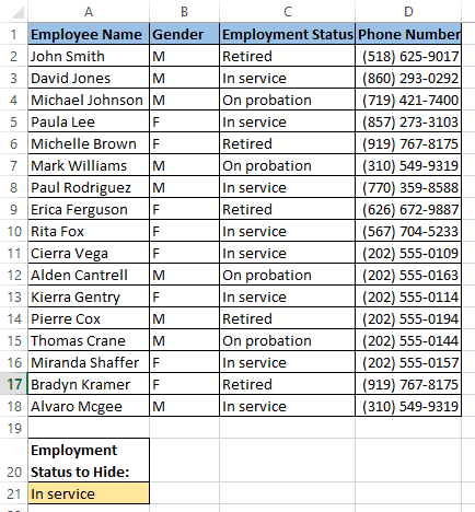
The only difference from the first dataset is that we have a value in cell A21 that will determine which rows should be hidden. So when cell A21 contains the value ‘Retired’ then only the rows containing the Employment Status ‘Retired’ are hidden.
Similarly, when cell A21 contains the value ‘On probation’ then only the rows containing the Employment Status ‘On probation’ are hidden.
When there is nothing in cell A21, we want all rows to be displayed.
We want this to happen in real-time, every time the value in cell A21 changes. For this, we need to make use of Excel’s Worksheet_SelectionChange function.
The Worksheet_SelectionChange Event
The Worksheet_SelectionChange procedure is an Excel built-in VBA event
It comes pre-installed with the worksheet and is called whenever a user selects a cell and then changes his/her selection to some other cell.
Since this function comes pre-installed with the worksheet, you need to place it in the code module of the correct sheet so that you can use it.
In our code, we are going to put all our lines inside this function, so that they get executed whenever the user changes the value in A21 and then selects some other cell.
Writing the VBA Code
Here’s the code that we are going to use:
To enter the above code, you need to copy it and paste it in your developer window, inside your worksheet’s Worksheet_SelectionChange procedure. Here’s how:
- From the Developer menu ribbon, select Visual Basic.
- Once your VBA window opens, you will see all your project files and folders in the Project Explorer on the left side.
- In the Project Explorer, double click on the name of your worksheet, under the VBA project with the same name as your Excel workbook. In our example, we are working with Sheet1.
- This will open up a new module window for your selected sheet.
- Click on the dropdown arrow on the left of the window. You should see an option that says ‘Worksheet’.
- Click on the ‘Worksheet’ option. By default, you will see the Worksheet_SelectionChange procedure created for you in the module window.
- Now you can start coding. Copy the above lines of code and paste them into the Worksheet_SelectionChange procedure, right after the line: Private Sub Worksheet_SelectionChange(ByVal Target As Range).
- Close the VBA window.


Running the Macro
The Worksheet_SelectionChange procedure starts running as soon as you are done coding. So you don’t need to explicitly run the macro for it to start working.
Try typing the ‘Retired’ in the cell A21, then clicking any other cell. You should find all rows containing the value ‘Retired’ in column C disappear.

Now try replacing the value in cell A21 to ‘On probation’, then clicking any other cell. You should find all rows containing the value ‘On probation’ in column C disappear.

Now try removing the value in cell A21 and leaving it empty. Then click on any other cell. You should find both rows become visible again.

This means the code is working in real-time when changes are made to cell B20.
Explanation of the Code
Let us take a few minutes to understand this code now.
- Lines 1, 2, and 3 define variables to hold the starting row and ending row of the dataset as well as the index of the criteria column. You can change the values according to your requirement.
- Lines 4 to 10, loop through each cell in column “3” (or column C) of the worksheet. If the cell contains the value in cell A21, then we set the ‘Hidden’ attribute of the entire row (corresponding to that cell) to True, which means we want to hide the entire corresponding row.
In this way, the above code hides the rows of the dataset depending on the value in cell A21. If A21 does not contain any value then the code displays all rows.
In this tutorial, I showed you how you can use Filters as well as Excel VBA to hide rows based on a cell value.
I did this with the help of two simple examples – one that removes required rows only when the macro is explicitly run and another that works in real-time.
I hope that we have been successful in helping you understand the concept behind the code so that you can customize it and use it in your own applications.
Other Excel tutorials you may also like:
Источник
Working with large datasets that contain rows after rows of data can be quite painful.
In such cases, looking for data that match particular criteria can be like looking for a needle in a haystack.
Thankfully, Excel provides some features that let you hide certain rows based on the cell value so that you only see the rows that you want to see. There are two ways to do this:
- Using filters
- Using VBA
In this tutorial, we will discuss both methods, and you can pick the method you feel most comfortable with.
Using Filters to Hide Rows based on Cell Value
Let us say you have the dataset shown below, and you want to see data about only those employees who are still in service.
This is really easy to do using filters. Here are the steps you need to follow:
- Select the working area of your dataset.
- From the Data tab, select the Filter button. You will find it in the ‘Sort and Filter’ group.

- You should now see a small arrow button on every cell of the header row.

- These buttons are meant to help you filter your cells. You can click on any arrow to choose a filter for the corresponding column.
- In this example, we want to filter out the rows that contain the Employment status = “In service”. So, select the arrow next to the Employment Status header.
- Uncheck the boxes next to all the statuses, except “In service”. You can simply uncheck “Select All” to quickly uncheck everything and then just select “In service”.

- Click OK.
You should now be able to see only the rows with Employment Status=”In service”. All other rows should now be hidden.
Note: To unhide the hidden cells, simply click on the Filter button again.
Using VBA to Hide Rows based on Cell Value
The second method requires a little coding. If you are accustomed to using macros and a little coding using VBA, then you get much more scope and flexibility to manipulate your data to behave exactly the way you want.
Writing the VBA Code
The following code will help you display only the rows that contain information about employees who are ‘In service’ and will hide all other rows:
Sub HideRows()
StartRow = 2
EndRow = 19
ColNum = 3
For i = StartRow To EndRow
If Cells(i, ColNum).Value <> "In service" Then
Cells(i, ColNum).EntireRow.Hidden = True
Else
Cells(i, ColNum).EntireRow.Hidden = False
End If
Next i
End Sub
The macro loops through each cell of column C and hide the rows that do not contain the value “In service”. It should essentially analyze each cell from rows 2 to 19 and adjust the ‘Hidden’ attribute of the row that you want to hide.
To enter the above code, copy it and paste it into your developer window. Here’s how:
- From the Developer menu ribbon, select Visual Basic.

- Once your VBA window opens, you will see all your files and folders in the Project Explorer on the left side. If you don’t see Project Explorer, click on View->Project Explorer.

- Make sure ‘ThisWorkbook’ is selected under the VBA project with the same name as your Excel workbook.
- Click Insert->Module. You should see a new module window open up.

- Now you can start coding. Copy the above lines of code and paste them into the new module window.

- In our example, we want to hide the rows that do not contain the value ‘In service’ in column 3. But you can replace the value of ColNum number from “3” in line 4 to the column number containing your criteria values.
- Close the VBA window.
Note: If your dataset covers more than 19 rows, you can change the values of the StartRow and EndRow variables to your required row numbers.
If you can’t see the Developer ribbon, from the File menu, go to Options. Select Customize Ribbon and check the Developer option from Main Tabs.
Finally, Click OK.
Your macro is now ready to use.
Running the Macro
Whenever you need to use the above macro, all you need to do is run it, and here’s how:
- Select the Developer tab
- Click on the Macros button (under the Code group).
- This will open the Macro Window, where you will find the names of all the macros that you have created so far.
- Select the macro (or module) named ‘HideRows’ and click on the Run button.

You should see all the rows where Employment Status is not ’In service’ hidden.
Explanation of the Code
Here’s a line by line explanation of the above code:
- In line 1 we defined the function name.
Sub HideRows()
- In lines 2, 3 and 4 we defined variables to hold the starting row and ending row of the dataset as well as the index of the criteria column.
StartRow = 2
EndRow = 19
ColNum = 3
- In lines 5 to 11, we looped through each cell in column “3” (or column C) of the Active Worksheet. If a cell does not contain the value “Inservice”, then we set the ‘Hidden’ attribute of the entire row (corresponding to that cell) to True, which means we want to hide the entire corresponding row.
For i = StartRow To EndRow
If Cells(i, ColNum).Value <> "In service" Then
Cells(i, ColNum).EntireRow.Hidden = True
Else
Cells(i, ColNum).EntireRow.Hidden = False
End If
Next i
- Line 12 simply demarcates the end of the HideRows function.
End Sub
In this way, the above code hides all the rows that do not contain the value ‘In service’ in column C.
Un-hiding Columns Based On Cell Value
Now that we have been able to successfully hide unwanted rows, what if we want to see the hidden rows again?
Doing this is quite easy. You only need to make a small change to the HideRows function.
Sub UnhideRows()
StartRow = 2
EndRow = 19
ColNum = 3
For i = StartRow To EndRow
Cells(i, ColNum).EntireRow.Hidden = False
Next i
End Sub
Here, we simply ensured that irrespective of the value, all the rows are displayed (by setting the Hidden property of all rows to False).
You can run this macro in exactly the same way as HideRows.
Hiding Rows Based On Cell Values in Real-Time
In the first example, the columns are hidden only when the macro runs. However, most of the time, we want to hide columns on-the-fly, based on the value in a particular cell.
So, let’s now take a look at another example that demonstrates this. In this example, we have the following dataset:
The only difference from the first dataset is that we have a value in cell A21 that will determine which rows should be hidden. So when cell A21 contains the value ‘Retired’ then only the rows containing the Employment Status ‘Retired’ are hidden.
Similarly, when cell A21 contains the value ‘On probation’ then only the rows containing the Employment Status ‘On probation’ are hidden.
When there is nothing in cell A21, we want all rows to be displayed.
We want this to happen in real-time, every time the value in cell A21 changes. For this, we need to make use of Excel’s Worksheet_SelectionChange function.
The Worksheet_SelectionChange Event
The Worksheet_SelectionChange procedure is an Excel built-in VBA event
It comes pre-installed with the worksheet and is called whenever a user selects a cell and then changes his/her selection to some other cell.
Since this function comes pre-installed with the worksheet, you need to place it in the code module of the correct sheet so that you can use it.
In our code, we are going to put all our lines inside this function, so that they get executed whenever the user changes the value in A21 and then selects some other cell.
Writing the VBA Code
Here’s the code that we are going to use:
StartRow = 2
EndRow = 19
ColNum = 3
For i = StartRow To EndRow
If Cells(i, ColNum).Value = Range("A21").Value Then
Cells(i, ColNum).EntireRow.Hidden = True
Else
Cells(i, ColNum).EntireRow.Hidden = False
End If
Next i
To enter the above code, you need to copy it and paste it in your developer window, inside your worksheet’s Worksheet_SelectionChange procedure. Here’s how:
- From the Developer menu ribbon, select Visual Basic.
- Once your VBA window opens, you will see all your project files and folders in the Project Explorer on the left side.
- In the Project Explorer, double click on the name of your worksheet, under the VBA project with the same name as your Excel workbook. In our example, we are working with Sheet1.
- This will open up a new module window for your selected sheet.
- Click on the dropdown arrow on the left of the window. You should see an option that says ‘Worksheet’.

- Click on the ‘Worksheet’ option. By default, you will see the Worksheet_SelectionChange procedure created for you in the module window.
- Now you can start coding. Copy the above lines of code and paste them into the Worksheet_SelectionChange procedure, right after the line: Private Sub Worksheet_SelectionChange(ByVal Target As Range).

- Close the VBA window.
Running the Macro
The Worksheet_SelectionChange procedure starts running as soon as you are done coding. So you don’t need to explicitly run the macro for it to start working.
Try typing the ‘Retired’ in the cell A21, then clicking any other cell. You should find all rows containing the value ‘Retired’ in column C disappear.
Now try replacing the value in cell A21 to ‘On probation’, then clicking any other cell. You should find all rows containing the value ‘On probation’ in column C disappear.
Now try removing the value in cell A21 and leaving it empty. Then click on any other cell. You should find both rows become visible again.
This means the code is working in real-time when changes are made to cell B20.
Explanation of the Code
Let us take a few minutes to understand this code now.
- Lines 1, 2, and 3 define variables to hold the starting row and ending row of the dataset as well as the index of the criteria column. You can change the values according to your requirement.
StartRow = 2
EndRow = 19
ColNum = 3
- Lines 4 to 10, loop through each cell in column “3” (or column C) of the worksheet. If the cell contains the value in cell A21, then we set the ‘Hidden’ attribute of the entire row (corresponding to that cell) to True, which means we want to hide the entire corresponding row.
For i = StartRow To EndRow
If Cells(i, ColNum).Value = Range("A21").Value Then
Cells(i, ColNum).EntireRow.Hidden = True
Else
Cells(i, ColNum).EntireRow.Hidden = False
End If
Next i
In this way, the above code hides the rows of the dataset depending on the value in cell A21. If A21 does not contain any value then the code displays all rows.
In this tutorial, I showed you how you can use Filters as well as Excel VBA to hide rows based on a cell value.
I did this with the help of two simple examples – one that removes required rows only when the macro is explicitly run and another that works in real-time.
I hope that we have been successful in helping you understand the concept behind the code so that you can customize it and use it in your own applications.
Other Excel tutorials you may also like:
- How to Hide Columns Based On Cell Value in Excel
- How to Delete Filtered Rows in Excel (with and without VBA)
- How to Highlight Every Other Row in Excel (Conditional Formatting & VBA)
- How to Unhide All Rows in Excel with VBA
- How to Set a Row to Print on Every Page in Excel
- How to Paste in a Filtered Column Skipping the Hidden Cells
- How to Select Multiple Rows in Excel
- How to Select Rows with Specific Text in Excel
- How to Move Row to Another Sheet Based On Cell Value in Excel?
- How to Compare Two Cells in Excel?
Watch Video – How to Hide Zero Values in Excel + How to Remove Zero Values
In case you prefer reading over watching a video, below is the complete written tutorial.
Sometimes in Excel, you may want to hide zero values in your dataset and show these cells as blanks.
Suppose you have a dataset as shown below and you want to hide the value 0 in all these cells (or want to replace it with something such as a dash or the text ‘Not Available’).
While you can do this manually with a small dataset, you’ll need better ways when working with large datasets.
In this tutorial, I will show you multiple ways to hide zero values in Excel and one method to select and remove all the zero values from the dataset.
Important Note: When you hide a 0 in a cell using the methods shown in this tutorial, it will only hide the 0 and not remove it. While the cells may look empty, those cells still contain the 0s. And in case you use these cells (that have hidden zeroes) in any formula, these will be used in the formula.
Let’s get started and dive into each of these methods!
Automatically Hide Zero Value in Cells
Excel has an inbuilt functionality that allows you to automatically hide all the zero values for the entire worksheet.
All you have to do is uncheck a box in Excel options, and the change will be applied to the entire worksheet.
Suppose you have the sales dataset as shown below and you want to hide all the zero values and show a blank cells instead.
Below are the steps to hide zeros from all the cells in a workbook in Excel:
- Open the workbook in which you want to hide all the zeros
- Click the File tab

- Click on Options

- In the Excel Options dialog box that opens, click on the ‘Advanced’ option in the left pane

- Scroll down to the section that says ‘Display option for this worksheet’, and select the worksheet in which you want to hide the zeros.

- Uncheck the ‘Show a zero in cells that have zero value’ option

- Click Ok


The above steps would instantly hide zeros in all the cells in the selected worksheet.
This change is also applied to cells where zero is a result of a formula.
Remember that this method only hides the 0 value in the cells and doesn’t remove these. The 0 is still there, it’s just hidden.
This is the best and fastest method to hide zero values in Excel. But this is useful only if you want to hide zero values in the entire worksheet. In case you only want this to hide zero values in a specific range of cells, it’s better to use other methods covered next in this tutorial.
Hide Zero Value in Cells using Conditional Formatting
While the above method is the most convenient one, it doesn’t allow you to hide zeros only in a specific range (rather it hides zero values in the entire worksheet).
In case you only want to hide zeros for a specific dataset (or multiple datasets), you can use conditional formatting.
With conditional formatting, you can apply a specific format based on the value in the cells. So, if the value in some cells is 0, you can simply program conditional formatting to hide it (or even highlight it if you want).
Suppose you have a dataset as shown below and you want to hide zeros in the cells.
Below are the steps to hide zeros in Excel using conditional formatting:
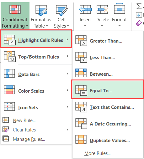
- Select the dataset
- Click the ‘Home’ tab

- In the ‘Styles’ group, click on ‘Conditional Formatting’.

- Place the cursor over the ‘Highlight Cells Rules’ options and in the options that show up, click on the ‘Equal to’ option.

- In the ‘Equal To’ dialog box, enter ‘0’ in the left field.

- Select the Format drop-down and click on ‘Custom Format’.

- In the ‘Format Cells’ dialog box, select the ‘Font’ tab.
- From the Color drop-down, choose the white color.

- Click OK.
- Click OK.


The above steps change the font color of the cells that have the zeros to white, which make these cells look blank.
This workaround works only when you have a white background in your worksheet. In case there is any other background-color in the cells, the white color may still keep the zeros visible.
In case you want to truly hide the zeros in the cells, where the cells look blank no matter what background color is given to the cells, you can use the steps below.
- Select the dataset
- Click the ‘Home’ tab
- In the ‘Styles’ group, click on ‘Conditional Formatting’.
- Place the cursor over the ‘Highlight Cells Rules’ options and in the options that show up, click on the ‘Equal to’ option.
- In the ‘Equal To’ dialog box, enter 0 in the left field.
- Select the Format drop-down and click on Custom Format.
- In the ‘Format Cells’ dialog box, select the ‘Number’ tab and click on the ‘Custom’ option in the left pane.
- In the Custom format option, enter the following in the Type field: ;;; (three semi-colons without space)
- Click OK.
- Click OK.

The above steps change the custom formatting of cells that have the value 0.
When you use three semi-colons as the format, it hides everything in the cell (be it numeric or text). And since this format is applied only to those cells which have the value 0 in it, it only hides the zeros and not the rest of the dataset.
You can also use this method to highlight these cells in a different color (such as red or yellow). To do this, just add another step (after Step  where you need to select the Fill tab in the ‘Format cells’ dialog box and then select the color in which you want to highlight the cells.
Both the methods covered above also work when 0 is a result of a formula in a cell.
Note: Both the method covered in this section only hide the zero values. It doesn’t remove these zeros. This means that in case you use these cells in calculations, all the zeros will be used as well.
Hide Zero Value using Custom Formatting
Another way to hide zero values from a dataset is by creating a custom format that hides the value in cells that have 0s, while any other value is displayed as expected.
Below are the steps to use a custom format to hide zeros in cells:
- Select the entire dataset for which you want to apply this format. If you want this for the entire worksheet, select all the cells
- With the cells selected, click the Home tab
- In the Cells group, click the Format option

- From the drop-down option, click on Format Cells. This will open the Format cells dialog box

- In the Format Cells dialog box, select the Number tab

- In the option on the left pane, click on the Custom option.
- In the options on the right, enter the following format in the Type field: 0;-0;;@
- Click OK


The above steps would apply a custom format to the selected cells where only those cells which have the value 0 are formatted to hide the value, while the rest of the cells display the data as expected.
How does this custom format work?
In Excel, there are four types of data formats that you specify:
- Positive numbers
- Negative numbers
- Zeros
- Text
And for each of these data types, you can specify a format.
In most cases, there is a default format – General, which keeps all these data types visible. But you have the flexibility of creating a specific format for each of these data types.
Below is the custom format structure you need to follow in case you are applying a custom format to each of these data types:
<Positive Numbers>;<Negative Numbers>;<Zeros>;<Text>
In the method covered above, I have specified the format to:
0;-0;;@
The above format does the following:
- Positive numbers are shown as is
- Negative numbers are shown with a negative sign
- Zeros are hidden (as no format is specified)
- Text is shown as is
Replace Zeros with Dash or Some Specific Text
In some cases, you may want to not just hide the zeros in the cells, but replace these with something more meaning.
For example, you may want to remove the zeros and replace it with a dash or a text such as “Not Available” or “Data Yet to Come”
This is again made possible using custom number formatting, where you can specify what a cell should display instead of a zero.
Below are the steps to convert a 0 to a dash in Excel:
- Select the entire dataset for which you want to apply this format. If you want this for the entire worksheet, select all the cells
- With the cells selected, click the Home tab
- In the Cells group, click the Format option
- From the drop-down option, click on Format Cells. This will open the Format cells dialog box
- In the Format Cells dialog box, select the Number tab
- In the option on the left pane, click on the Custom option.
- In the options on the right, enter the following format in the Type field: 0;-0;–;@

- Click OK

The above steps would keep all the other cells as is and change the cells with the value 0 to show a dash (–).
Note: In this example, I have chosen to replace the zero with a dash, but you can use any text as well. For example, if you want to show the NA in the cells, you can use the following format: 0;-0;”NA”;@
Pro Tip: You can also specify a few text colors in custom number formatting. For example, if you want the cells with zeros to show the text NA in red color, you can use the following format: 0;-0;[Red]”NA”;@
Hide Zero Values in Pivot Tables
There can be two scenarios where a Pivot Table shows the value as 0:
- The source data cells that are summarized in the Pivot Table has 0 values
- The source data cells that are summarized in the Pivot Table are blanks and the Pivot table has been formatted to show the empty cells as zero
Let’s see how to hide the zeros in the Pivot table in each scenario:
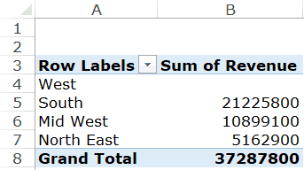
When Source Data cells have 0s
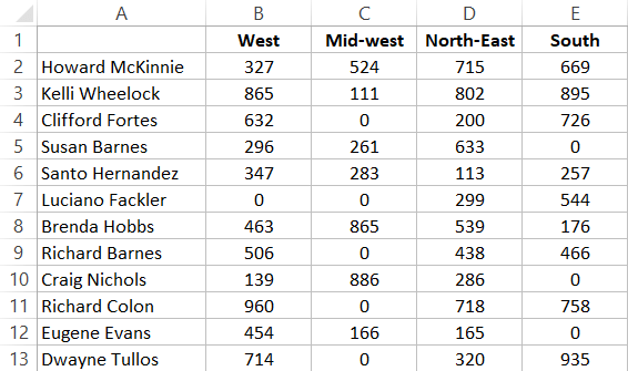
Below is a sample dataset that I have used to create a Pivot table. Note that the Quantity/Revenue/Profit numbers for all the records for ‘West’ are 0.
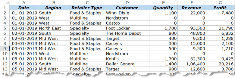
The Pivot table created using this data set looks as shown below:
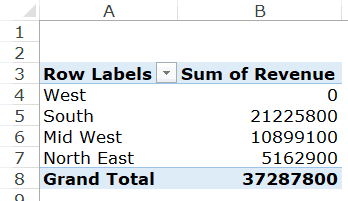
Since there were 0s in the dataset for all the records for West region, you see a 0 in the Pivot table for west here.
If you want to hide zero in this Pivot Table, you can use conditional formatting to do this.
However, conditional formatting in the Pivot Table in Excel works a little different than regular data.
Here are the steps to apply conditional formatting to Pivot Table to hide zeros:
- Select any cell in the column that has 0s in the Pivot Table summary (Do not select all the cells, but only one cell)
- Click the Home tab
- In the ‘Styles’ group, click on ‘Conditional Formatting’.
- Place the cursor over the ‘Highlight Cells Rules’ options and in the options that show up, click on the ‘Equal to’ option.
- In the ‘Equal To’ dialog box, enter 0 in the left field.
- Select the Format drop-down and click on Custom Format.
- In the ‘Format Cells’ dialog box, select the Number tab and click on the ‘Custom’ option in the left pane.
- In the Custom format option, enter the following in the Type field: ;;; (three semi-colons without space)
- Click OK. You will see small Formatting Options icon at the right of the selected cell.
- Click on this ‘Formatting Options’ icon

- In the options that become available, choose – All cells showing “Sum of Revenue” values for “Region”.


The above steps hide the zero in the Pivot Table in such a way that if you change the Pivot Table structure (by adding more rows/columns headers to it, the zeros will continue to be hidden).
If you want to learn more about how this works, here is a detailed tutorial on the right way to apply conditional formatting to Pivot Tables.
When Source Data cells have empty cells
Below is an example where I have a dataset that has empty cells for all the records for West.
If I create a Pivot Table using this data, I will get the result as shown below.
By default, the Pivot Table shows you empty cells when all the cells in the source data are blank. But in case you still see a 0 in this case, follow the below steps to hide the zero and show blank cells:
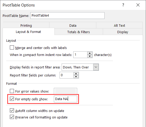
- Right-click on any of the cells in the Pivot Table
- Click on ‘Pivot Table Options’

- In the ‘PivotTable Options’ dialog box, click on the ‘Layout & Format’ tab
- In the Format options, check the options and ‘For empty cells show:’ and leave it blank.

- Click OK.


The above steps would hide the zeros in the Pivot Table and show a blank cell instead.
In case you want the Pivot Table to show something instead of the 0, you can specify that in step 4. For example, if you want to show the text – ‘Data not Available’, instead of the 0, type this text in the field (as shown below).
Find and Remove Zeros in Excel
In all the methods above, I have shown you ways to hide the 0 value in the cell, but the value still remains in the cell.
In case you want to remove the zero values from the dataset (which would leave you with blank cells), use the below steps:
- Select the dataset (or the entire worksheet)
- Click the Home tab
- In the ‘Editing’ group, click on ‘Find & Select’
- In the options that are shown in the drop-down, click on ‘Replace’

- In the ‘Find and Replace’ dialog box, make the following changes:
- In the ‘Find what’ field, enter 0
- In the ‘Replace with’ field, enter nothing (leave it empty)
- Click on Options button and check the ‘Match entire cell contents’ option

- Click on Replace All


The above steps would instantly replace all the cells that had zero value with a blank.
In case you don’t want to remove the zeros right away and first select the cells, use the following steps:
- Select the dataset (or the entire worksheet)
- Click the Home tab
- In the ‘Editing’ group, click on ‘Find & Select’
- In the options that are shown in the drop-down, click on ‘Replace’
- In the ‘Find and Replace’ dialog box, make the following changes:
- In the ‘Find what’ field, enter 0
- In the ‘Replace with’ field, enter nothing (leave it empty)
- Click on Options button and check the ‘Match entire cell contents’ option
- Click on the ‘Find All’ button. This will give you a list of all the cells that have 0 in it
- Press Control-A (hold the control key and press A). This will select all the cells that have 0 in it.


Now, that you have all the cells with 0 selected, you can delete these, replace these with something else, or change the color and highlight these.
Hiding the Zeros Vs. Removing The Zeros
When treating the cells with 0s in it, you need to know the difference between hiding these and removing these.
When you hide the zero value in a cell, it is not visible to you, but it still remains in the cell. This means that if you have a dataset and you use it for calculation, that 0 value will also be used in the calculation.
On the contrary, when you have a blank cell, using it in formulas may mean that Excel automatically ignores these cells (depending on which formula you’re using).
For example, below is what I get when I use the AVERAGE formula to get the average for two columns (the result is in row 14). Column A has cells where the 0 value has been hidden (but is still there in the cell) and Column B has cells where the 0 value has been removed.
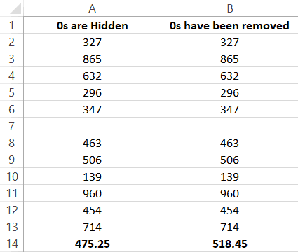
You can see the difference in the result despite the fact that the dataset for both datasets looks the same.
This happens as the AVERAGE formula ignores blank cells in column B, but it uses the ones in Column A (as the ones in column A still has the value 0 in it).
You may also like the following Excel tutorials:
- How to Hide a Worksheet in Excel
- Delete Rows Based on a Cell Value
- Delete Blank Rows in Excel
- How to Delete Every Other Row in Excel (or Every Nth Row)
- Show Formulas in Excel Instead of the Values
- Change Negative Number to Positive in Excel
- How to Remove Leading Zeros in Excel
How can I hide the data in an individual cell I want to keep private? Hiding the confidential content of a cell is a useful trick most Excel users probably don’t know. In this tutorial we’ll walk you through the procedure to hide data or text in a cell in Excel 2016.
How to Hide Data or Text in an Excel Cell?
- Open your Excel spreadsheet in Excel 2016.
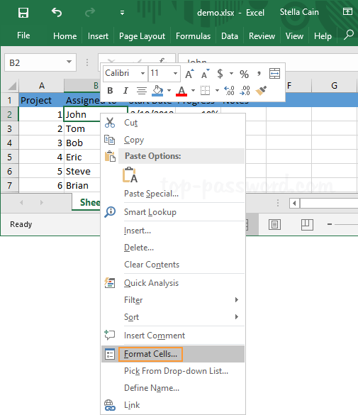
- Select the cells that contain sensitive data you want to hide. Right-click to choose “Format Cells” option from the drop-down menu.

- On the Number tab, choose the Custom category and enter three semicolons (;;;) without the parentheses into the Type box.

- Click OK and now the data in your selected cells is hidden.

This method only hides the cell contents from being seen. The contents are still there and accessible for formulas, charts as such. If you want to display the hidden cell values, right-click the cells and select “Format Cells“. But this time choose “General” as the format of the cells.
Now, the hidden text in your cells will be visible again.
- Previous Post: How to Hide / Unhide Entire Row or Column in Excel 2016
- Next Post: How to Change Text to Uppercase or Lowercase in Excel 2016
-
03-18-2009, 11:20 AM
#1
Forum Contributor
How to hide #VALUE! in cells ????
Hi,
There are empty cells in a column.
Where the cells are empty, they are reading #VALUE! because I have copied down a formula in all other cells above and below etc.
Is there any quick way of making the #VALUE! disappear or by hiding?
(Other than the copied formulas in the column, there are also conditional formatting so when the numbers drop below zero value, it turns the numbers red).
It’s a long sheet and I want to avoid deleting each #VALUE! by hand !
Thanks.
Last edited by NBVC; 03-18-2009 at 04:00 PM.
-
03-18-2009, 11:24 AM
#2
Re: How to hide #VALUE! in cells ????
Hi,
You have two options.
If you haven’t used all three Conditional formats (assuming XL 2003 or less) then you could format the font to be white if there’s an error. Otherwise why not just wrap the formula in an IF(ISERROR(yourformula),»»,yourformula)
HTH
Richard Buttrey
RIP — d. 06/10/2022
If any of the responses have helped then please consider rating them by clicking the small star icon
below the post.
-
03-18-2009, 11:24 AM
#3
Re: How to hide #VALUE! in cells ????
I dont know which formula you are using by using — operator we can suppress #value in many cases eg
=sumproduct(—(conditon) , —( condition2) , etc ))
-
03-18-2009, 11:24 AM
#4
Re: How to hide #VALUE! in cells ????
Can you tell us the formula in the cell?
-
03-18-2009, 11:29 AM
#5
Forum Contributor
Re: How to hide #VALUE! in cells ????
Firstly, thanks for replying so promptly.
The formula is quite basic and reads:
=F2071-J2071
-
03-18-2009, 11:33 AM
#6
Forum Contributor
Re: How to hide #VALUE! in cells ????
Just added in an additional conditional format with the following:
=IF(ISERROR(F2072-J2072),»»,F2072-J2072)
Doesn’t appear to have worked ?
Thanks.
-
03-18-2009, 12:13 PM
#7
Forum Contributor
Re: How to hide #VALUE! in cells ????
Can somebody help please…………….. gotta get this roted urgently.
Thanks.
-
03-18-2009, 12:23 PM
#8
Forum Contributor
Re: How to hide #VALUE! in cells ????
Originally Posted by Richard Buttrey
Hi,
You have two options.
If you haven’t used all three Conditional formats (assuming XL 2003 or less) then you could format the font to be white if there’s an error. Otherwise why not just wrap the formula in an IF(ISERROR(yourformula),»»,yourformula)
HTH
Richard — see below — any thoughts ?
Thanks.
-
03-18-2009, 12:30 PM
#9
Re: How to hide #VALUE! in cells ????
How about?
=IF(SUM(F2072,J2072),F2072-J2072,»»)
Where there is a will there are many ways.
If you are happy with the results, please add to the contributor’s reputation by clicking the reputation icon (star icon) below left corner
Please also mark the thread as Solved once it is solved. Check the FAQ’s to see how.
-
03-18-2009, 12:31 PM
#10
Re: How to hide #VALUE! in cells ????
Hi,
can u post a sample of ur workbook..
may be u are calculating a numeric field but there are some text data in them.. (in the form of white space in front of the number)
-
03-18-2009, 12:33 PM
#11
Re: How to hide #VALUE! in cells ????
-
03-18-2009, 12:33 PM
#12
Re: How to hide #VALUE! in cells ????
I would suggest
=IF(COUNT(F2072,J2072)=2,F2072-J2072,»»)
Calculation only undertaken if both values are numbers.
-
03-18-2009, 02:07 PM
#13
Forum Contributor
Re: How to hide #VALUE! in cells ????
Well done — this worked.
You’re life savers.
Thanks.
-
08-20-2013, 03:59 AM
#14
Registered User
Re: How to hide #VALUE! in cells ????
Try this Hopefully it works…
=IF(ISERROR(F2072-J2072),»Message»)
-
08-20-2013, 04:10 AM
#15
Re: How to hide #VALUE! in cells ????


 below the post.
