Value if true value if false excel - Word и Excel - помощь в работе с программами

IF function

The IF function is one of the most popular functions in Excel, and it allows you to make logical comparisons between a value and what you expect.

So an IF statement can have two results. The first result is if your comparison is True, the second if your comparison is False.

For example, =IF(C2=”Yes”,1,2) says IF(C2 = Yes, then return a 1, otherwise return a 2).

Use the IF function, one of the logical functions, to return one value if a condition is true and another value if it’s false.

IF(logical_test, value_if_true, [value_if_false])

For example:

=IF(A2>B2,»Over Budget»,»OK»)
=IF(A2=B2,B4-A4,»»)

Argument name	Description
logical_test (required)	The condition you want to test.
value_if_true (required)	The value that you want returned if the result of *logical_test* is TRUE.
value_if_false (optional)	The value that you want returned if the result of *logical_test* is FALSE.

Simple IF examples

=IF(C2=”Yes”,1,2)

In the above example, cell D2 says: IF(C2 = Yes, then return a 1, otherwise return a 2)

=IF(C2=1,”Yes”,”No”)

In this example, the formula in cell D2 says: IF(C2 = 1, then return Yes, otherwise return No)As you see, the IF function can be used to evaluate both text and values. It can also be used to evaluate errors. You are not limited to only checking if one thing is equal to another and returning a single result, you can also use mathematical operators and perform additional calculations depending on your criteria. You can also nest multiple IF functions together in order to perform multiple comparisons.

=IF(C2>B2,”Over Budget”,”Within Budget”)

In the above example, the IF function in D2 is saying IF(C2 Is Greater Than B2, then return “Over Budget”, otherwise return “Within Budget”)

=IF(C2>B2,C2-B2,0)

In the above illustration, instead of returning a text result, we are going to return a mathematical calculation. So the formula in E2 is saying IF(Actual is Greater than Budgeted, then Subtract the Budgeted amount from the Actual amount, otherwise return nothing).

=IF(E7=”Yes”,F5*0.0825,0)

In this example, the formula in F7 is saying IF(E7 = “Yes”, then calculate the Total Amount in F5 * 8.25%, otherwise no Sales Tax is due so return 0)

Note: If you are going to use text in formulas, you need to wrap the text in quotes (e.g. “Text”). The only exception to that is using TRUE or FALSE, which Excel automatically understands.

Common problems

Problem	What went wrong
0 (zero) in cell	There was no argument for either value_if_true or value_if_False arguments. To see the right value returned, add argument text to the two arguments, or add TRUE or FALSE to the argument.
#NAME? in cell	This usually means that the formula is misspelled.

Need more help?

You can always ask an expert in the Excel Tech Community or get support in the Answers community.

Что возвращает функция

Заданное вами значение при выполнении двух условий ИСТИНА или ЛОЖЬ.

Синтаксис

=IF(logical_test, [value_if_true], [value_if_false]) — английская версия

=ЕСЛИ(лог_выражение; [значение_если_истина]; [значение_если_ложь]) — русская версия

Аргументы функции

logical_test (лог_выражение) — это условие, которое вы хотите протестировать. Этот аргумент функции должен быть логичным и определяемым как ЛОЖЬ или ИСТИНА. Аргументом может быть как статичное значение, так и результат функции, вычисления;
[value_if_true] ([значение_если_истина]) — (не обязательно) — это то значение, которое возвращает функция. Оно будет отображено в случае, если значение которое вы тестируете соответствует условию ИСТИНА;
[value_if_false] ([значение_если_ложь]) — (не обязательно) — это то значение, которое возвращает функция. Оно будет отображено в случае, если условие, которое вы тестируете соответствует условию ЛОЖЬ.

Дополнительная информация

В функции ЕСЛИ может быть протестировано 64 условий за один раз;
Если какой-либо из аргументов функции является массивом — оценивается каждый элемент массива;
Если вы не укажете условие аргумента FALSE (ЛОЖЬ) value_if_false (значение_если_ложь) в функции, т.е. после аргумента value_if_true (значение_если_истина) есть только запятая (точка с запятой), функция вернет значение “0”, если результат вычисления функции будет равен FALSE (ЛОЖЬ).
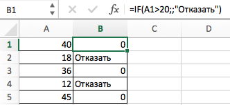
На примере ниже, формула =IF(A1> 20,”Разрешить”) или =ЕСЛИ(A1>20;»Разрешить») , где value_if_false (значение_если_ложь) не указано, однако аргумент value_if_true (значение_если_истина) по-прежнему следует через запятую. Функция вернет “0” всякий раз, когда проверяемое условие не будет соответствовать условиям TRUE (ИСТИНА).

|
Если вы не укажете условие аргумента TRUE(ИСТИНА) (value_if_true (значение_если_истина)) в функции, т.е. условие указано только для аргумента value_if_false (значение_если_ложь), то формула вернет значение “0”, если результат вычисления функции будет равен TRUE (ИСТИНА);
На примере ниже формула равна =IF (A1>20;«Отказать») или =ЕСЛИ(A1>20;»Отказать»), где аргумент value_if_true (значение_если_истина) не указан, формула будет возвращать “0” всякий раз, когда условие соответствует TRUE (ИСТИНА).

Функция Если в Excel примеры с несколькими условиями

Пример 1. Проверяем простое числовое условие с помощью функции IF (ЕСЛИ)

При использовании функции ЕСЛИ в Excel, вы можете использовать различные операторы для проверки состояния. Вот список операторов, которые вы можете использовать:

Ниже приведен простой пример использования функции при расчете оценок студентов. Если сумма баллов больше или равна «35», то формула возвращает “Сдал”, иначе возвращается “Не сдал”.

Пример 2. Использование вложенной функции IF (ЕСЛИ) для проверки условия выражения

Функция может принимать до 64 условий одновременно. Несмотря на то, что создавать длинные вложенные функции нецелесообразно, то в редких случаях вы можете создать формулу, которая множество условий последовательно.

В приведенном ниже примере мы проверяем два условия.

Первое условие проверяет, сумму баллов не меньше ли она чем 35 баллов. Если это ИСТИНА, то функция вернет “Не сдал”;
В случае, если первое условие — ЛОЖЬ, и сумма баллов больше 35, то функция проверяет второе условие. В случае если сумма баллов больше или равна 75. Если это правда, то функция возвращает значение “Отлично”, в других случаях функция возвращает “Сдал”.

Пример 3. Вычисляем сумму комиссии с продаж с помощью функции IF (ЕСЛИ) в Excel

Функция позволяет выполнять вычисления с числами. Хороший пример использования — расчет комиссии продаж для торгового представителя.

В приведенном ниже примере, торговый представитель по продажам:

не получает комиссионных, если объем продаж меньше 50 тыс;
получает комиссию в размере 2%, если продажи между 50-100 тыс
получает 4% комиссионных, если объем продаж превышает 100 тыс.

Рассчитать размер комиссионных для торгового агента можно по следующей формуле:

=IF(B2<50,0,IF(B2<100,B2*2%,B2*4%)) — английская версия

=ЕСЛИ(B2<50;0;ЕСЛИ(B2<100;B2*2%;B2*4%)) — русская версия

В формуле, использованной в примере выше, вычисление суммы комиссионных выполняется в самой функции ЕСЛИ. Если объем продаж находится между 50-100K, то формула возвращает B2 * 2%, что составляет 2% комиссии в зависимости от объема продажи.

Больше лайфхаков в нашем Telegram Подписаться

Пример 4. Используем логические операторы (AND/OR) (И/ИЛИ) в функции IF (ЕСЛИ) в Excel

Вы можете использовать логические операторы (AND/OR) (И/ИЛИ) внутри функции для одновременного тестирования нескольких условий.

Например, предположим, что вы должны выбрать студентов для стипендий, основываясь на оценках и посещаемости. В приведенном ниже примере учащийся имеет право на участие только в том случае, если он набрал более 80 баллов и имеет посещаемость более 80%.

Вы можете использовать функцию AND (И) вместе с функцией IF (ЕСЛИ), чтобы сначала проверить, выполняются ли оба эти условия или нет. Если условия соблюдены, функция возвращает “Имеет право”, в противном случае она возвращает “Не имеет право”.

Формула для этого расчета:

=IF(AND(B2>80,C2>80%),”Да”,”Нет”) — английская версия

=ЕСЛИ(И(B2>80;C2>80%);»Да»;»Нет») — русская версия

Пример 5. Преобразуем ошибки в значения “0” с помощью функции IF (ЕСЛИ)

С помощью этой функции вы также можете убирать ячейки содержащие ошибки. Вы можете преобразовать значения ошибок в пробелы или нули или любое другое значение.

Формула для преобразования ошибок в ячейках следующая:

=IF(ISERROR(A1),0,A1) — английская версия

=ЕСЛИ(ЕОШИБКА(A1);0;A1) — русская версия

Формула возвращает “0”, в случае если в ячейке есть ошибка, иначе она возвращает значение ячейки.

ПРИМЕЧАНИЕ. Если вы используете Excel 2007 или версии после него, вы также можете использовать функцию IFERROR для этого.

Точно так же вы можете обрабатывать пустые ячейки. В случае пустых ячеек используйте функцию ISBLANK, на примере ниже:

=IF(ISBLANK(A1),0,A1) — английская версия

=ЕСЛИ(ЕПУСТО(A1);0;A1) — русская версия

Источник

The IF function runs a logical test and returns one value for a TRUE result, and another value for a FALSE result. The result from IF can be a value, a cell reference, or even another formula. By combining the IF function with other logical functions like AND and OR, you can test more than one condition at a time.

Syntax

The generic syntax for the IF function looks like this:

=IF(logical_test,[value_if_true],[value_if_false])

The first argument, logical_test, is typically an expression that returns either TRUE or FALSE. The second argument, value_if_true, is the value to return when logical_test is TRUE. The last argument, value_if_false, is the value to return when logical_test is FALSE. Both value_if_true and value_if_false are optional, but you must provide one or the other. For example, if cell A1 contains 80, then:

=IF(A1>75,TRUE) // returns TRUE
=IF(A1>75,"OK") // returns "OK"
=IF(A1>85,"OK") // returns FALSE
=IF(A1>75,10,0) // returns 10
=IF(A1>85,10,0) // returns 0
=IF(A1>75,"Yes","No") // returns "Yes"
=IF(A1>85,"Yes","No") // returns "No"

Notice that text values like «OK», «Yes», «No», etc. must be enclosed in double quotes («»). However, numeric values should not be enclosed in quotes.

Logical tests

The IF function supports logical operators (>,<,<>,=) when creating logical tests. Most commonly, the logical_test in IF is a complete logical expression that will evaluate to TRUE or FALSE. The table below shows some common examples:

Goal	Logical test
If A1 is greater than 75	A1>75
If A1 equals 100	A1=100
If A1 is less than or equal to 100	A1<=100
If A1 equals «Red»	A1=»red»
If A1 is not equal to «Red»	A1<>»red»
If A1 is less than B1	A1<B1
If A1 is empty	A1=»»
If A1 is not empty	A1<>»»
If A1 is less than current date	A1<TODAY()

Notice text values must be enclosed in double quotes («»), but numbers do not. The IF function does not support wildcards, but you can combine IF with COUNTIF to get basic wildcard functionality. To test for substrings in a cell, you can use the IF function with the SEARCH function.

Pass or Fail example

In the worksheet shown above, we want to assign either «Pass» or «Fail» based on a test score. A passing score is 70 or higher. The formula in D6, copied down, is:

=IF(C5>=70,"Pass","Fail")

Translation: If the value in C5 is greater than or equal to 70, return «Pass». Otherwise, return «Fail».

Note that the logical flow of this formula can be reversed. This formula returns the same result:

=IF(C5<70,"Fail","Pass")

Translation: If the value in C5 is less than 70, return «Fail». Otherwise, return «Pass».

Both formulas above, when copied down, will return correct results.

Note: If you are new to the idea of formula criteria, this article explains many examples.

Assign points based on color

In the worksheet below, we want to assign points based on the color in column B. If the color is «red», the result should be 100. If the color is «blue», the result should be 125. This requires that we use a formula based on two IF functions, one nested inside the other. The formula in C5, copied down, is:

=IF(B5="red",100,IF(B5="blue",125))

Translation: IF the value in B5 is «red», return 100. Else, if the value in B5 is «blue», return 125.

There are three things to notice in this example:

The formula will return FALSE if the value in B5 is anything except «red» or «blue»
The text values «red» and «blue» must be enclosed in double quotes («»)
The IF function is not case-sensitive and will match «red», «Red», «RED», or «rEd».

This is a simple example of a nested IFs formula. See below for a more complex example.

Return another formula

The IF function can return another formula as a result. For example, the formula below will return A1*5% when A1 is less than 100, and A1*7% when A1 is greater than or equal to 100:

=IF(A1<100,A1*5%,A1*7%)

Nested IF statements

The IF function can be «nested». A «nested IF» refers to a formula where at least one IF function is nested inside another in order to test for more conditions and return more possible results. Each IF statement needs to be carefully «nested» inside another so that the logic is correct. For example, the following formula can be used to assign a grade rather than a pass / fail result:

=IF(C6<70,"F",IF(C6<75,"D",IF(C6<85,"C",IF(C6<95,"B","A"))))

Up to 64 IF functions can be nested. However, in general, you should consider other functions, like VLOOKUP or XLOOKUP for more complex scenarios, because they can handle more conditions in a more streamlined fashion. For a more details see this article on nested IFs.

Note: the newer IFS function is designed to handle multiple conditions without nesting. However, a lookup function like VLOOKUP or XLOOKUP is usually a better approach unless the logic for each condition is custom.

IF with AND, OR, NOT

The IF function can be combined with the AND function and the OR function. For example, to return «OK» when A1 is between 7 and 10, you can use a formula like this:

=IF(AND(A1>7,A1<10),"OK","")

Translation: if A1 is greater than 7 and less than 10, return «OK». Otherwise, return nothing («»).

To return B1+10 when A1 is «red» or «blue» you can use the OR function like this:

=IF(OR(A1="red",A1="blue"),B1+10,B1)

Translation: if A1 is red or blue, return B1+10, otherwise return B1.

=IF(NOT(A1="red"),B1+10,B1)

Translation: if A1 is NOT red, return B1+10, otherwise return B1.

IF cell contains specific text

Because the IF function does not support wildcards, it is not obvious how to configure IF to check for a specific substring in a cell. A common approach is to combine the ISNUMBER function and the SEARCH function to create a logical test like this:

=ISNUMBER(SEARCH(substring,A1)) // returns TRUE or FALSE

For example, to check for the substring «xyz» in cell A1, you can use a formula like this:

=IF(ISNUMBER(SEARCH("xyz",A1)),"Yes","No")

Read a detailed explanation here.

More information

Read more about nested IFs
Learn how to use VLOOKUP instead of nested IFs (video)
50 Examples of formula criteria

Notes

The IF function is not case-sensitive.
To count values conditionally, use the COUNTIF or the COUNTIFS functions.
To sum values conditionally, use the SUMIF or the SUMIFS functions.
If any of the arguments to IF are supplied as arrays, the IF function will evaluate every element of the array.

Источник

The logical IF statement in Excel is used for the recording of certain conditions. It compares the number and / or text, function, etc. of the formula when the values correspond to the set parameters, and then there is one record, when do not respond — another.

Logic functions — it is a very simple and effective tool that is often used in practice. Let us consider it in details by examples.

The syntax of the function «IF» with one condition

The operation syntax in Excel is the structure of the functions necessary for its operation data.

=IF(boolean;value_if_TRUE;value_if_FALSE)

Let us consider the function syntax:

Boolean – what the operator checks (text or numeric data cell).
Value_if_TRUE – what will appear in the cell when the text or numbers correspond to a predetermined condition (true).
Value_if_FALSE – what appears in the box when the text or the number does not meet the predetermined condition (false).

Example:

Logical IF functions.

The operator checks the A1 cell and compares it to 20. This is a «Boolean». When the contents of the column is more than 20, there is a true legend «greater 20». In the other case it’s «less or equal 20».

Attention! The words in the formula need to be quoted. For Excel to understand that you want to display text values.

Here is one more example. To gain admission to the exam, a group of students must successfully pass a test. The results are listed in a table with columns: a list of students, a credit, an exam.

list.

The statement IF should check not the digital data type but the text. Therefore, we prescribed in the formula В2= «done» We take the quotes for the program to recognize the text correctly.

The function IF in Excel with multiple conditions

Usually one condition for the logic function is not enough. If you need to consider several options for decision-making, spread operators’ IF into each other. Thus, we get several functions IF in Excel.

The syntax is as follows:

Here the operator checks the two parameters. If the first condition is true, the formula returns the first argument is the truth. False — the operator checks the second condition.

Examples of a few conditions of the function IF in Excel:

It’s a table for the analysis of the progress. The student received 5 points:

А – excellent;
В – above average or superior work;
C – satisfactory;
D – a passing grade;
E – completely unsatisfactory.

IF statement checks two conditions: the equality of value in the cells.

In this example, we have added a third condition, which implies the presence of another report card and «twos». The principle of the operator is the same.

Enhanced functionality with the help of the operators «AND» and «OR»

When you need to check out a few of the true conditions you use the function И. The point is: IF A = 1 AND A = 2 THEN meaning в ELSE meaning с.

OR function checks the condition 1 or condition 2. As soon as at least one condition is true, the result is true. The point is: IF A = 1 OR A = 2 THEN value B ELSE value C.

Functions AND & OR can check up to 30 conditions.

An example of using the operator AND:

It’s the example of using the logical operator OR.

How to compare data in two tables

Users often need to compare the two spreadsheets in an Excel to match. Examples of the «life»: compare the prices of goods in different bringing, to compare balances (accounting reports) in a few months, the progress of pupils (students) of different classes, in different quarters, etc.

To compare the two tables in Excel, you can use the COUNTIFS statement. Consider the order of application functions.

For example, consider the two tables with the specifications of various food processors. We planned allocation of color differences. This problem in Excel solves the conditional formatting.

Baseline data (tables, which will work with):

tables.

Select the first table. Conditional Formatting — create a rule — use a formula to determine the formatted cells:

In the formula bar write: = COUNTIFS (comparable range; first cell of first table)=0. Comparing range is in the second table.

To drive the formula into the range, just select it first cell and the last. «= 0» means the search for the exact command (not approximate) values.

Choose the format and establish what changes in the cell formula in compliance. It’s better to do a color fill.

Select the second table. Conditional Formatting — create a rule — use the formula. Use the same operator (COUNTIFS). For the second table formula:

Download all examples in Excel

Now it is easy to compare the characteristics of the data in the table.

Источник

How to Use the IF Function in Excel: Step-by-Step (2023)

The IF function is going to be one of the most useful functions of Excel you’ll ever come across🤩

Once you know how to write the IF function, you’ll use it almost everywhere. With the IF function, Excel tests a given condition.

And returns one value if the condition turns true and another if it turns false. More details about the IF function with many examples of the same await you in the guide below 👇

So jump straight in and take our free sample workbook along with you to practice better.

How to use the IF function in Excel

The IF function is a logical function of Excel that’ll test a supplied condition. If the condition is true, the IF function would return one value.

And if it is false, it will return another value. And by the way, both these values will be supplied by you. Let’s see this through an example 👩‍🏫

Here we have a list of some people along with their ages.

Can we use the IF function to see which of these are of the age of 50? For sure. See here:

Activate a cell.
Write the IF function as below:

= IF (B2=50,

For the first argument of the IF function, write in the condition to be tested 👴

We want to test if the age of each person equals 50. Ages are in column B so we have written the logical condition B2=50.

This tells Excel to test if B2 is equal to 50.

Note that we have used a logical operator (=) to specify the condition. You’d need a logical operator to specify any kind of condition.

Kasper Langmann, Microsoft Office Specialist

As the next argument, write the value_if_true as below:

= IF (B2=50, “Equals 50”,

The value_if_true is the value that Excel would return if the logical condition turned true. It is an optional argument that you can omit ❌

For now, we are setting it to “Equals 50”.

If the value_if_true is omitted, and the logical test turns true, Excel simply returns the Boolean value “TRUE” in its place.

Kasper Langmann, Microsoft Office Specialist

Next, write in the value_if_false as below:

= IF (B2=50, “Equals 50”, “Doesn’t equal 50”)

The value_if_false is the value that Excel would return if the logical condition turned false. It is also an optional argument that you can omit.

We have set it to ‘Doesn’t Equal 50” 🙈

Do not forget to enclose the value_if_true and value_if_false in double quotation marks. Or else would fail to recognize it as a text.

And your IF function would return the #NAME error 🤯

If the value_if_false is omitted, Excel simply returns the Boolean value “FALSE” in its place.

Kasper Langmann, Microsoft Office Specialist

All good! Hit Enter.

The IF function evaluates if Cell B2 is equal to 50. And as that’s not the case, we get “Doesn’t equal 50” (the value_if_false) 🚩

Drag and drop the same formula to the whole list.

And there you get the results of the IF function for the entire list🥂

Note how Excel has supplied the value if true (Equals 50) for Cell B3 and B6 where the age is 60. Pretty simple that was!

IF and logical operators

You can take the IF function game levels ahead by using it together with logical operators.

For example, using the same dataset as above, can we readily see which people are above 50 👀

Write the IF function as below:

= IF (B2>50,

The logical condition for the IF function

As we want to find the ages that are greater than 50, we are going to define a logical condition using the greater than (>) logical operator.

So we have written the condition as B2>50 (is B2 greater than 50?).

Then write the value_if_true and value_if_false as below:

= IF (B2>50, “Greater than 50”, “Not greater than 50”)

We want Excel to return the text string “Greater than 50” if the age is more than 50.

And if any age is less than 50, we want Excel to return “Not greater than 50” ✈

Press Enter.

The IF function evaluates if Cell B2 is greater than 50. And we get the result “Greater than 50” in the very first cell as the age in Cell B2 is 88. (88>50) 👌

Drag and drop the same formula to the whole list.

Excel evaluates the whole list, and we have our results ready. You can use logical operators like that to test any logical condition.

Pro Tip!

You can use a total of 6 logical operators to write any logical test in Excel 6️⃣

Equal to (=)
Greater than (>)
Less than (<)
Greater than or equal to (>=)
Less than or equal to (<=)
Not equal to (<>)

Other IF formula examples

We’ve yet not had enough of the IF function – and there’s much more to come. Let’s see some more examples of the IF function below 🚴‍♀️

IF formula example #1

The above two examples show how you can use the IF function with numbers. But what if you want to use it with text?

You can still do that. Look into the data below.

Some employees worked overtime, whereas others did not. Based on the overtime detail, we need to offer incentives to employees 💰

So can we readily see which employees are getting a bonus this time?

Write the IF function as below:

= IF (B2=”Worked Overtime”

As we want to find which employee did overtime, we defined the logical condition B2=” Worked Overtime”.

This way Excel will see if cell B2 contains the text value “Worked Overtime” or not.

Here’s something for you to take note of. As we have specified text in our logical condition this time, we have enclosed it in double quotation marks.

Excel would fail to test a text logical condition if the text portion is not enclosed in quotation marks 📌

Kasper Langmann, Microsoft Office Specialist

Then write the value_if_true and value_in_false as below:

= IF (B2=”Worked Overtime”, “Yes”, “No”)

For any employee who has worked overtime, Excel will return a “Yes” and vice versa.

Hit Enter to run the function 🏃‍♀️

Drag and drop the same formula to the whole list.

The IF function tests if the cells have the text value “Worked Overtime”. And for all the cells that have this value, the result is a “Yes”. And for the employees who didn’t work overtime, the result is a “No”.

Pro Tip!

Did you note that Cell B5 has the status “WORKED OVERTIME” (uppercase characters)?

However, the IF function still finds the logical test to be true, and we have the value “Yes”.

This tells that the IF function is not case-sensitive 🏆

IF formula example #2

This example is going to be an interesting one. We are going to use the IF function with dates in logical tests.

The image below shows different events scheduled on certain dates 📅

In addition to these events, there is another event planned for 03 March 2023. We will now use the IF function to see if any event clashes with the event on 03 March.

Write the IF function as below:

= IF (B2=DATE(2023,03,03)

We have written the logical test as B2=DATE(2023,03,03)

Excel would now test if cell B2 contains the date 03-Mar-2022 or not.

Pro Tip!

To write the logical criterion using date, we have used the DATE function that works as follows:

=DATE(year,mm,dd)

It is important to know that the logical functions of Excel cannot recognize dates. They instead consider them as text strings 😅

To use dates in the IF function, you must use the DATE function for Excel to convert the date into an understandable format.

Alternatively, you can convert the date into a serial number and then write the IF function like this:

= IF (B2=44988,

However, to know the serial number for the targeted date (like 44988 for 03 March 2023), you still need to apply the DATE function separately 🤷‍♀️

Then write the value_if_true and value_if_false as below:

= IF (B2=DATE(2023,03,03), “Yes”, “No”)

For events that are scheduled on 03 March 2022, Excel will return a “Yes”.

And if that’s not the case, we will get a clean “No” ❌

Interesting, right? Let’s now run the function to see the final results.

Hit Enter.

IF function evaluates the corresponding value

Drag and drop the same formula to the whole list.

Seems like we would have to miss out on Event 3 and Event 5 🙅‍♂️

That’s it – Now what?

A long way we’ve come. In the guide above, we have seen how to use the basic IF function, IF function with logical operators, and with single and multiple conditions.

With this, you now know all the ins and outs of the IF function of Excel. I hope you enjoyed reading it as much as I enjoyed writing it ✍

If you found the IF function useful, must know that it only makes one function of the great Excel. This giant spreadsheet software has so much more for you to explore.

To become an Excel maestro, you must have a fine grip on Excel functions. Particularly, the key Excel functions like the VLOOKUP, SUMIF, and IF functions.

Don’t know where to start? Enroll in my 30-minute free email course that will take you through these (and many more) functions of Excel.

Frequently asked questions

IF is a logical function of Excel. It tests a given condition to be logically true or false.

It allows users to specify a value to be returned if the supplied condition is true, and a value if it is false.

The IF function then evaluates the condition and returns the relevant value if it proves true or false.

The Excel IF function has the following three articles:

Logical_test (required argument) – this is the logical test to be performed.

Value_if_true (optional argument) – this is the value to be returned if the logical test is true.

Value_if_false (optional argument) – this is the value to be returned if the logical test is false.

The IF function can be used to test more complex scenarios by nesting multiple IF functions together.

For example, you can nest multiple IF functions together as follows:

= IF (logical_condition, [value_if_true], IF (logical_condition, [value_if_true], [value_if_false])

This tells Excel to test the first IF function and return the value_if_true if it is true. And if it is false, test the second (nested) IF function.

To learn this in much more detail (with a handful of examples), read our tutorial on the Nested IF function here!

Kasper Langmann2023-02-23T14:47:57+00:00

Page load link

Источник

This Excel tutorial explains how to use the Excel IF function with syntax and examples.

Description

The Microsoft Excel IF function returns one value if the condition is TRUE, or another value if the condition is FALSE.

The IF function is a built-in function in Excel that is categorized as a Logical Function. It can be used as a worksheet function (WS) in Excel. As a worksheet function, the IF function can be entered as part of a formula in a cell of a worksheet.

If you want to follow along with this tutorial, download the example spreadsheet.

Download Example

Syntax

The syntax for the IF function in Microsoft Excel is:

IF( condition, value_if_true, [value_if_false] )

Parameters or Arguments

condition: The value that you want to test.
value_if_true: It is the value that is returned if condition evaluates to TRUE.
value_if_false: Optional. It is the value that is returned if condition evaluates to FALSE.

Returns

The IF function returns value_if_true when the condition is TRUE.
The IF function returns value_if_false when the condition is FALSE.
The IF function returns FALSE if the value_if_false parameter is omitted and the condition is FALSE.

Example (as Worksheet Function)

Let’s explore how to use the IF function as a worksheet function in Microsoft Excel.

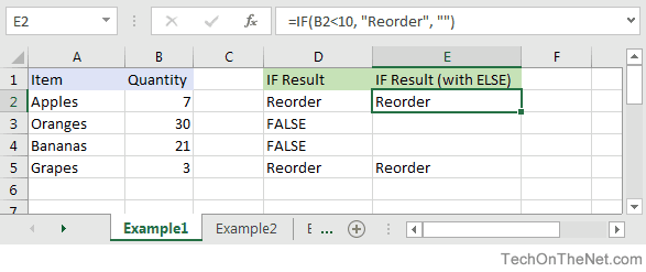
Based on the Excel spreadsheet above, the following IF examples would return:

=IF(B2<10, "Reorder", "")
Result: "Reorder"

=IF(A2="Apples", "Equal", "Not Equal")
Result: "Equal"

=IF(B3>=20, 12, 0)
Result: 12

Combining the IF function with Other Logical Functions

Quite often, you will need to specify more complex conditions when writing your formula in Excel. You can combine the IF function with other logical functions such as AND, OR, etc. Let’s explore this further.

AND function

The IF function can be combined with the AND function to allow you to test for multiple conditions. When using the AND function, all conditions within the AND function must be TRUE for the condition to be met. This comes in very handy in Excel formulas.

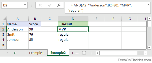
Based on the spreadsheet above, you can combine the IF function with the AND function as follows:

=IF(AND(A2="Anderson",B2>80), "MVP", "regular")
Result: "MVP"

=IF(AND(B2>=80,B2<=100), "Great Score", "Not Bad")
Result: "Great Score"

=IF(AND(B3>=80,B3<=100), "Great Score", "Not Bad")
Result: "Not Bad"

=IF(AND(A2="Anderson",A3="Smith",A4="Johnson"), 100, 50)
Result: 100

=IF(AND(A2="Anderson",A3="Smith",A4="Parker"), 100, 50)
Result: 50

In the examples above, all conditions within the AND function must be TRUE for the condition to be met.

OR function

The IF function can be combined with the OR function to allow you to test for multiple conditions. But in this case, only one or more of the conditions within the OR function needs to be TRUE for the condition to be met.

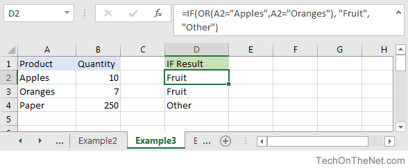
Based on the spreadsheet above, you can combine the IF function with the OR function as follows:

=IF(OR(A2="Apples",A2="Oranges"), "Fruit", "Other")
Result: "Fruit"

=IF(OR(A4="Apples",A4="Oranges"),"Fruit","Other")
Result: "Other"

=IF(OR(A4="Bananas",B4>=100), 999, "N/A")
Result: 999

=IF(OR(A2="Apples",A3="Apples",A4="Apples"), "Fruit", "Other")
Result: "Fruit"

In the examples above, only one of the conditions within the OR function must be TRUE for the condition to be met.

Let’s take a look at one more example that involves ranges of percentages.

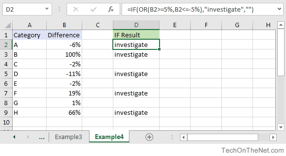
Based on the spreadsheet above, we would have the following formula in cell D2:

=IF(OR(B2>=5%,B2<=-5%),"investigate","")
Result: "investigate"

This IF function would return «investigate» if the value in cell B2 was either below -5% or above 5%. Since -6% is below -5%, it will return «investigate» as the result. We have copied this formula into cells D3 through D9 to show you the results that would be returned.

For example, in cell D3, we would have the following formula:

=IF(OR(B3>=5%,B3<=-5%),"investigate","")
Result: "investigate"

This formula would also return «investigate» but this time, it is because the value in cell B3 is greater than 5%.

Frequently Asked Questions

Question: In Microsoft Excel, I’d like to use the IF function to create the following logic:

if C11>=620, and C10=»F»or»S», and C4<=$1,000,000, and C4<=$500,000, and C7<=85%, and C8<=90%, and C12<=50, and C14<=2, and C15=»OO», and C16=»N», and C19<=48, and C21=»Y», then reference cell A148 on Sheet2. Otherwise, return an empty string.

Answer: The following formula would accomplish what you are trying to do:

=IF(AND(C11>=620, OR(C10="F",C10="S"), C4<=1000000, C4<=500000, C7<=0.85, C8<=0.9, C12<=50, C14<=2, C15="OO", C16="N", C19<=48, C21="Y"), Sheet2!A148, "")

Question: In Microsoft Excel, I’m trying to use the IF function to return 0 if cell A1 is either < 150,000 or > 250,000. Otherwise, it should return A1.

Answer: You can use the OR function to perform an OR condition in the IF function as follows:

=IF(OR(A1<150000,A1>250000),0,A1)

In this example, the formula will return 0 if cell A1 was either less than 150,000 or greater than 250,000. Otherwise, it will return the value in cell A1.

Question: In Microsoft Excel, I’m trying to use the IF function to return 25 if cell A1 > 100 and cell B1 < 200. Otherwise, it should return 0.

Answer: You can use the AND function to perform an AND condition in the IF function as follows:

=IF(AND(A1>100,B1<200),25,0)

In this example, the formula will return 25 if cell A1 is greater than 100 and cell B1 is less than 200. Otherwise, it will return 0.

Question: In Microsoft Excel, I need to write a formula that works this way:

IF (cell A1) is less than 20, then times it by 1,
IF it is greater than or equal to 20 but less than 50, then times it by 2
IF its is greater than or equal to 50 and less than 100, then times it by 3
And if it is great or equal to than 100, then times it by 4

Answer: You can write a nested IF statement to handle this. For example:

=IF(A1<20, A1*1, IF(A1<50, A1*2, IF(A1<100, A1*3, A1*4)))

Question: In Microsoft Excel, I need a formula in cell C5 that does the following:

IF A1+B1 <= 4, return $20
IF A1+B1 > 4 but <= 9, return $35
IF A1+B1 > 9 but <= 14, return $50
IF A1+B1 >= 15, return $75

Answer: In cell C5, you can write a nested IF statement that uses the AND function as follows:

=IF((A1+B1)<=4,20,IF(AND((A1+B1)>4,(A1+B1)<=9),35,IF(AND((A1+B1)>9,(A1+B1)<=14),50,75)))

Question: In Microsoft Excel, I need a formula that does the following:

IF the value in cell A1 is BLANK, then return «BLANK»
IF the value in cell A1 is TEXT, then return «TEXT»
IF the value in cell A1 is NUMERIC, then return «NUM»

Answer: You can write a nested IF statement that uses the ISBLANK function, the ISTEXT function, and the ISNUMBER function as follows:

=IF(ISBLANK(A1)=TRUE,"BLANK",IF(ISTEXT(A1)=TRUE,"TEXT",IF(ISNUMBER(A1)=TRUE,"NUM","")))

Question: In Microsoft Excel, I want to write a formula for the following logic:

IF R1<0.3 AND R2<0.3 AND R3<0.42 THEN «OK» OTHERWISE «NOT OK»

Answer: You can write an IF statement that uses the AND function as follows:

=IF(AND(R1<0.3,R2<0.3,R3<0.42),"OK","NOT OK")

Question: In Microsoft Excel, I need a formula for the following:

IF cell A1= PRADIP then value will be 100
IF cell A1= PRAVIN then value will be 200
IF cell A1= PARTHA then value will be 300
IF cell A1= PAVAN then value will be 400

Answer: You can write an IF statement as follows:

=IF(A1="PRADIP",100,IF(A1="PRAVIN",200,IF(A1="PARTHA",300,IF(A1="PAVAN",400,""))))

Question: In Microsoft Excel, I want to calculate following using an «if» formula:

if A1<100,000 then A1*.1% but minimum 25
and if A1>1,000,000 then A1*.01% but maximum 5000

Answer: You can write a nested IF statement that uses the MAX function and the MIN function as follows:

=IF(A1<100000,MAX(25,A1*0.1%),IF(A1>1000000,MIN(5000,A1*0.01%),""))

Question: In Microsoft Excel, I am trying to create an IF statement that will repopulate the data from a particular cell if the data from the formula in the current cell equals 0. Below is my attempt at creating an IF statement that would populate the data; however, I was unsuccessful.

=IF(IF(ISERROR(M24+((L24-S24)/AA24)),"0",M24+((L24-S24)/AA24)))=0,L24)

The initial part of the formula calculates the EAC (Estimate At completion = AC+(BAC-EV)/CPI); however if the current EV (Earned Value) is zero, the EAC will equal zero. IF the outcome is zero, I would like the BAC (Budget At Completion), currently recorded in another cell (L24), to be repopulated in the current cell as the EAC.

Answer: You can write an IF statement that uses the OR function and the ISERROR function as follows:

=IF(OR(S24=0,ISERROR(M24+((L24-S24)/AA24))),L24,M24+((L24-S24)/AA24))

Question: I have been looking at your Excel IF, AND and OR sections and found this very helpful, however I cannot find the right way to write a formula to express if C2 is either 1,2,3,4,5,6,7,8,9 and F2 is F and F3 is either D,F,B,L,R,C then give a value of 1 if not then 0. I have tried many formulas but just can’t get it right, can you help please?

Answer: You can write an IF statement that uses the AND function and the OR function as follows:

=IF(AND(C2>=1,C2<=9, F2="F",OR(F3="D",F3="F",F3="B",F3="L",F3="R",F3="C")),1,0)

Question:In Excel, I have a roadspeed of a car in m/s in cell A1 and a drop down menu of different units in C1 (which unclude mph and kmh). I have used the following IF function in B1 to convert the number to the unit selected from the dropdown box:

=IF(C1="mph","=A1*2.23693629",IF(C1="kmh","A1*3.6"))

However say if kmh was selected B1 literally just shows A1*3.6 and does not actually calculate it. Is there away to get it to calculate it instead of just showing the text message?

Answer: You are very close with your formula. Because you are performing mathematical operations (such as A1*2.23693629 and A1*3.6), you do not need to surround the mathematical formulas in quotes. Quotes are necessary when you are evaluating strings, not performing math.

Try the following:

=IF(C1="mph",A1*2.23693629,IF(C1="kmh",A1*3.6))

Question:For an IF statement in Excel, I want to combine text and a value.

For example, I want to put an equation for work hours and pay. IF I am paid more than I should be, I want it to read how many hours I owe my boss. But if I work more than I am paid for, I want it to read what my boss owes me (hours*Pay per Hour).

I tried the following:

=IF(A2<0,"I owe boss" abs(A2) "Hours","Boss owes me" abs(A2)*15 "dollars")

Is it possible or do I have to do it in 2 separate cells? (one for text and one for the value)

Answer: There are two ways that you can concatenate text and values. The first is by using the & character to concatenate:

=IF(A2<0,"I owe boss " & ABS(A2) & " Hours","Boss owes me " & ABS(A2)*15 &  " dollars")

Or the second method is to use the CONCATENATE function:

=IF(A2<0,CONCATENATE("I owe boss ", ABS(A2)," Hours"), CONCATENATE("Boss owes me ", ABS(A2)*15,  " dollars"))

Question:I have Excel 2000. IF cell A2 is greater than or equal to 0 then add to C1. IF cell B2 is greater than or equal to 0 then subtract from C1. IF both A2 and B2 are blank then equals C1. Can you help me with the IF function on this one?

Answer: You can write a nested IF statement that uses the AND function and the ISBLANK function as follows:

=IF(AND(ISBLANK(A2)=FALSE,A2>=0),C1+A2, IF(AND(ISBLANK(B2)=FALSE,B2>=0),C1-B2, IF(AND(ISBLANK(A2)=TRUE, ISBLANK(B2)=TRUE),C1,"")))

Question:How would I write this equation in Excel? IF D12<=0 then D12*L12, IF D12 is > 0 but <=600 then D12*F12, IF D12 is >600 then ((600*F12)+((D12-600)*E12))

Answer: You can write a nested IF statement as follows:

=IF(D12<=0,D12*L12,IF(D12>600,((600*F12)+((D12-600)*E12)),D12*F12))

Question:In Excel, I have this formula currently:

=IF(OR(A1>=40, B1>=40, C1>=40), "20", (A1+B1+C1)-20)

If one of my salesman does sale for $40-$49, then his commission is $20; however if his/her sale is less (for example $35) then the commission is that amount minus $20 ($35-$20=$15). I have 3 columns that are needed based on the type of sale. Only one column per row will be needed. The problem is that, when left blank, the total in the formula cell is -20. I need help setting up this formula so that when the 3 columns are left blank, the cell with the formula is left blank as well.

Answer: Using the AND function and the ISBLANK function, you can write your IF statement as follows:

=IF(AND(ISBLANK(A1),ISBLANK(B1),ISBLANK(C1)),"",IF(OR(A1>40, B1>40, C1>40), "20", (A1+B1+C1)-20))

In this formula, we are using the ISBLANK function to check if all 3 cells A1, B1, and C1 are blank, and if they are return a blank value («»). Then the rest is the formula that you originally wrote.

Question:In Excel, I need to create a simple booking and and out system, that shows a date out and a date back

«A1» = allows person to input date booked out
«A2» =allows person to input date booked back in

«A3″= shows status of product, eg, booked out, overdue return etc.

I can automate A3 with the following IF function:

=IF(ISBLANK(A2),"booked out","returned")

But what I cant get to work is if the product is out for 10 days or more, I would like the cell to say «send email»

Can you assist?

Answer: Using the TODAY function and adding an additional IF function, you can write your formula as follows:

=IF(ISBLANK(A2),IF(TODAY()-A1>10,"send email","booked out"),"returned")

Question:Using Microsoft Excel, I need a formula in cell U2 that does the following:

IF the date in E2<=12/31/2010, return T2*0.75
IF the date in E2>12/31/2010 but <=12/31/2011, return T2*0.5
IF the date in E2>12/31/2011, return T2*0

I tried using the following formula, but it gives me «#VALUE!»

=IF(E2<=DATE(2010,12,31),T2*0.75), IF(AND(E2>DATE(2010,12,31),E2<=DATE(2011,12,31)),T2*0.5,T2*0)

Can someone please help? Thanks.

Answer: You were very close…you just need to adjust your parentheses as follows:

=IF(E2<=DATE(2010,12,31),T2*0.75, IF(AND(E2>DATE(2010,12,31),E2<=DATE(2011,12,31)),T2*0.5,T2*0))

Question:In Excel, I would like to add 60 days if grade is ‘A’, 45 days if grade is ‘B’ and 30 days if grade is ‘C’. It would roughly look something like this, but I’m struggling with commas, brackets, etc.

(IF C5=A)=DATE(YEAR(B5)+0,MONTH(B5)+0,DAY(B5)+60),
(IF C5=B)=DATE(YEAR(B5)+0,MONTH(B5)+0,DAY(B5)+45),
(IF C5=C)=DATE(YEAR(B5)+0,MONTH(B5)+0,DAY(B5)+30)

Answer:You should be able to achieve your date calculations with the following formula:

=IF(C5="A",B5+60,IF(C5="B",B5+45,IF(C5="C",B5+30)))

Question:In Excel, I am trying to write a function and can’t seem to figure it out. Could you help?

IF D3 is < 31, then 1.51
IF D3 is between 31-90, then 3.40
IF D3 is between 91-120, then 4.60
IF D3 is > 121, then 5.44

Answer:You can write your formula as follows:

=IF(D3>121,5.44,IF(D3>=91,4.6,IF(D3>=31,3.4,1.51)))

Question:I would like ask a question regarding the IF statement. How would I write in Excel this problem?

I have to check if cell A1 is empty and if not, check if the value is less than equal to 5. Then multiply the amount entered in cell A1 by .60. The answer will be displayed on Cell A2.

Answer:You can write your formula in cell A2 using the IF function and ISBLANK function as follows:

=IF(AND(ISBLANK(A1)=FALSE,A1<=5),A1*0.6,"")

Question:In Excel, I’m trying to nest an OR command and I can’t find the proper way to write it. I want the spreadsheet to do the following:

If D6 equals «HOUSE» and C6 equals either «MOUSE» or «CAT», I want to return the value in cell B6. Otherwise, the formula should return the value «BLANK».

I tried the following:

=IF((D6="HOUSE")*(C6="MOUSE")*OR(C6="CAT"));B6;"BLANK")

If I only ask for HOUSE and MOUSE or HOUSE and CAT, it works, but as soon as I ask for MOUSE OR CAT, it doesn’t work.

Answer:You can write your formula using the AND function and OR function as follows:

=IF(AND(D6="HOUSE",OR(C6="MOUSE",C6="CAT")),B6,"BLANK")

This will return the value in B6 if D6 equals «HOUSE» and C6 equals either «MOUSE» or «CAT». If those conditions are not met, the formula will return the text value of «BLANK».

Question:In Microsoft Excel, I’m trying to write the following formula:

If cell A1 equals «jaipur», «udaipur» or «jodhpur», then cell A2 should display «rajasthan»
If cell A1 equals «bangalore», «mysore» or «belgum», then cell A2 should display «karnataka»

Please help.

Answer:You can write your formula using the OR function as follows:

=IF(OR(A1="jaipur",A1="udaipur",A1="jodhpur"),"rajasthan", IF(OR(A1="bangalore",A1="mysore",A1="belgum"),"karnataka"))

This will return «rajasthan» if A1 equals either «jaipur», «udaipur» or «jodhpur» and it will return «karnataka» if A1 equals either «bangalore», «mysore» or «belgum».

Question:In Microsoft Excel I’m trying to achieve the following with IF function:

If a value in any cell in column F is «food» then add the value of its corresponding cell in column G (eg a corresponding cell for F3 is G3). The IF function is performed in another cell altogether. I can do it for a single pair of cells but I don’t know how to do it for an entire column. Could you help?

At the moment, I’ve got this:

=IF(F3="food"; G3; 0)

Answer:This formula can be created using the SUMIF formula instead of using the IF function:

=SUMIF(F1:F10,"=food",G1:G10)

This will evaluate the first 10 rows of data in your spreadsheet. You may need to adjust the ranges accordingly.

I notice that you separate your parameters with semi-colons, so you might need to replace the commas in the formula above with semi-colons.

Question:I’m looking for an Exel formula that says:

If F3 is «H» and E3 is «H», return 1
If F3 is «A» and E3 is «A», return 2
If F3 is «d» and E3 is «d», return 3

Appreciate if you can help.

Answer:This Excel formula can be created using the AND formula in combination with the IF function:

=IF(AND(F3="H",E3="H"),1,IF(AND(F3="A",E3="A"),2,IF(AND(F3="d",E3="d"),3,"")))

We’ve defaulted the formula to return a blank if none of the conditions above are met.

Question:I am trying to get Excel to check different boxes and check if there is text/numbers listed in the cells and then spit out «Complete» if all 5 Boxes have text/Numbers or «Not Complete» if one or more is empty. This is what I have so far and it doesn’t work.

=IF(OR(ISBLANK(J2),ISBLANK(M2),ISBLANK(R2),ISBLANK (AA2),ISBLANK (AB2)),"Not Complete","")

Answer:First, you are correct in using the ISBLANK function, however, you have a space between ISBLANK and (AA2), as well as ISBLANK and (AB2). This might seem insignificant, but Excel can be very picky and will return a #NAME? error. So first you need to eliminate those spaces.

Next, you need to change the ELSE condition of your IF function to return «Complete».

You should be able to modify your formula as follows:

=IF(OR(ISBLANK(J2),ISBLANK(M2),ISBLANK(R2),ISBLANK(AA2),ISBLANK(AB2)), "Not Complete", "Complete")

Now if any of the cell J2, M2, R2, AA2, or AB2 are blank, the formula will return «Not Complete». If all 5 cells have a value, the formula will return «Complete».

Question:I’m very new to the Excel world, and I’m trying to figure out how to set up the proper formula for an If/then cell.

What I’m trying for is:

If B2’s value is 1 to 5, then multiply E2 by .77
If B2’s value is 6 to 10, then multiply E2 by .735
If B2’s value is 11 to 19, then multiply E2 by .7
If B2’s value is 20 to 29, then multiply E2 by .675
If B2’s value is 30 to 39, then multiply E2 by .65

I’ve tried a few different things thinking I was on the right track based on the IF, and AND function tutorials here, but I can’t seem to get it right.

Answer:To write your IF formula, you need to nest multiple IF functions together in combination with the AND function.

The following formula should work for what you are trying to do:

=IF(AND(B2>=1, B2<=5), E2*0.77, IF(AND(B2>=6, B2<=10), E2*0.735, IF(AND(B2>=11, B2<=19), E2*0.7, IF(AND(B2>=20, B2<=29), E2*0.675, IF(AND(B2>=30, B2<=39), E2*0.65,"")))))

As one final component of your formula, you need to decide what to do when none of the conditions are met. In this example, we have returned «» when the value in B2 does not meet any of the IF conditions above.

Question:Here is the Excel formula that has me between a rock and a hard place.

If E45 <= 50, return 44.55
If E45 > 50 and E45 < 100, return 42
If E45 >=200, return 39.6

Again thank you very much.

Answer:You should be able to write this Excel formula using a combination of the IF function and the AND function.

The following formula should work:

=IF(E45<=50, 44.55, IF(AND(E45>50, E45<100), 42, IF(E45>=200, 39.6, "")))

Please note that if none of the conditions are met, the Excel formula will return «» as the result.

Question:I have a nesting OR function problem:

My nonworking formula is:

=IF(C9=1,K9/J7,IF(C9=2,K9/J7,IF(C9=3,K9/L7,IF(C9=4,0,K9/N7))))

In Cell C9, I can have an input of 1, 2, 3, 4 or 0. The problem is on how to write the «or» condition when a «4 or 0» exists in Column C. If the «4 or 0» conditions exists in Column C I want Column K divided by Column N and the answer to be placed in Column M and associated row

Answer:You should be able to use the OR function within your IF function to test for C9=4 OR C9=0 as follows:

=IF(C9=1,K9/J7,IF(C9=2,K9/J7,IF(C9=3,K9/L7,IF(OR(C9=4,C9=0),K9/N7))))

This formula will return K9/N7 if cell C9 is either 4 or 0.

Question:In Excel, I am trying to create a formula that will show the following:

If column B = Ross and column C = 8 then in cell AB of that row I want it to show 2013, If column B = Block and column C = 9 then in cell AB of that row I want it to show 2012.

Answer:You can create your Excel formula using nested IF functions with the AND function.

=IF(AND(B1="Ross",C1=8),2013,IF(AND(B1="Block",C1=9),2012,""))

This formula will return 2013 as a numeric value if B1 is «Ross» and C1 is 8, or 2012 as a numeric value if B1 is «Block» and C1 is 9. Otherwise, it will return blank, as denoted by «».

Question:In Excel, I really have a problem looking for the right formula to express the following:

If B1=0, C1 is equal to A1/2
If B1=1, C1 is equal to A1/2 times 20%
If D1=1, C1 is equal to A1/2-5

I’ve been trying to look for any same expressions in your site. Please help me fix this.

Answer:In cell C1, you can use the following Excel formula with 3 nested IF functions:

=IF(B1=0,A1/2, IF(B1=1,(A1/2)*0.2, IF(D1=1,(A1/2)-5,"")))

Please note that if none of the conditions are met, the Excel formula will return «» as the result.

Question:In Excel, I need the answer for an IF THEN statement which compares column A and B and has an «OR condition» for column C. My problem is I want column D to return yes if A1 and B1 are >=3 or C1 is >=1.

Answer:You can create your Excel IF formula as follows:

=IF(OR(AND(A1>=3,B1>=3),C1>=1),"yes","")

Please note that if none of the conditions are met, the Excel formula will return «» as the result.

Question:In Excel, what have I done wrong with this formula?

=IF(OR(ISBLANK(C9),ISBLANK(B9)),"",IF(ISBLANK(C9),D9-TODAY(), "Reactivated"))

I want to make an event that if B9 and C9 is empty, the value would be empty. If only C9 is empty, then the output would be the remaining days left between the two dates, and if the two cells are not empty, the output should be the string ‘Reactivated’.

The problem with this code is that IF(ISBLANK(C9),D9-TODAY() is not working.

Answer:First of all, you might want to replace your OR function with the AND function, so that your Excel IF formula looks like this:

=IF(AND(ISBLANK(C9),ISBLANK(B9)),"",IF(ISBLANK(C9),D9-TODAY(),"Reactivated"))

Next, make sure that you don’t have any abnormal formatting in the cell that contains the results. To be safe, right click on the cell that contains the formula and choose Format Cells from the popup menu. When the Format Cells window appears, select the Number tab. Choose General as the format and click on the OK button.

Question:I was wondering if you could tell me what I am doing wrong.
Here are the instructions:

A customer is eligible for a discount if the customer’s 2016 sales greater than or equal to 100000 OR if the customers First Order was placed in 2016.
If the customer qualifies for a discount, return a value of Y
If the customer does not qualify for a discount, return a value of N.

Here is the formula I’ve entered:

=IF(OR([2014 Sales]=0,[2015 Sales]=0,[2016 Sales]>=100000),"Y","N")

I only have 2 cells wrong. Can you help me please? I am very lost and confused.

Answer:You are very close with your IF formula, however, it looks like you need to add the AND function to your formula as follows:

=IF(OR([2016 Sales]>=100000,AND([2014 Sales]=0,[2015 Sales]=0),C8>=100000),"Y","N")

This formula should return Y if 2016 sales are greater than or equal to 100000, or if both 2014 sales and 2015 sales are 0. Otherwise, the formula will return N. You will also notice that we switched the order of your conditions in the formula so that it is easier to understand the formula based on your instructions above.

Question:Could you please help me? I need to use «OR» on my formula but I can’t get it to work. This is what I’ve tried:

=IF(C6>=0<=150,150000,IF(C6>=151<=160,158400))

Here is what I need the formula to do:

IF C6 IS >=0 OR <=150 THEN ASSIGN $150000

IF C6 IS >=151 OR <=160 THEN ASSIGN $158400

Answer:You should be able to use the AND function within your IF function as follows:

=IF(AND(ISBLANK(C6)=FALSE,C6>=0,C6<=150),150000,IF(AND(C6>=151,C6<=160),158400,""))

Notice that we first use the ISBLANK function to test C6 to make sure that it is not blank. This is because if C6 if blank, it will evalulate to greater than 0 and thus return 150000. To avoid this, we include ISBLANK(C6)=FALSE as one of the conditions in addition to C6>=0 and C6<=150. That way, you won’t return any false results if C6 is blank.

Question:I am having a problem with a formula, I want it to be IF E5=N then do the first formula, else do the second formula. Excel recognizes the =IF(logical_test,value_if_TRUE,value_if_FALSE) but doesn’t like the formula below:

=IF(e5="N",((AND(AH5-AG5<456, AH5-S5<822)), "Compliant", "not Compliant"),((AH5-S5<822), "Compliant", "not Compliant"))

Any help would be greatly appreciated.

Answer:To have the first formula executed when E5=N and then second formula executed when E5<>N, you will need to nest 2 additional IF functions within the main IF function as follows:

=IF(E5="N", IF((AND(AH5-AG5<456, AH5-S5<822)), "Compliant", "not Compliant"), IF((AH5-S5<822), "Compliant", "not Compliant"))

If E5=»N», the first nested IF function will be executed:

IF((AND(AH5-AG5<456, AH5-S5<822)), "Compliant", "not Compliant")

Otherwise,the second nested IF function will be executed:

IF((AH5-S5<822), "Compliant", "not Compliant"))

Question:I need to write a formula based on the following logic:

There is a maximum discount allowed of £1000 if the capital sum is less that £43000 and a lower discount of £500 if the capital sum is above £43000. So the formula should return either £500 or £1000 in the cell but the £43000 is made up of two numbers, say for e.g. £42750+350 and if the second number is less than the allowed discount, the actual lower value is returned — in this case the £500 or £1000 becomes £350. Or as another e.g. £42000+750 returns £750.

So on my spreadsheet, in this second e.g. I would have A1= £42000, A2=750, A3=A1+A2, A4=the formula with the changing discount, in this case £750.

How can I write this formula?

Answer:In cell A4, you can calculate the correct discount using the IF function and the MIN function as follows:

=IF(A3<43000, MIN(A2,1000), MIN(A2,500))

If A3 is less than 43000, the formula will return the lower value of A2 and 1000. Otherwise, it will return the lower value of A2 and 500.

Question: I have a list of sizes in column A with sizes 100, 200, 300, 400, 500, 600. Then I have another column B, with sizes of my products, and it is random, for example, 318, 445, 527. What I’m trying to create is for a value of 318 in column B, I need to return 400 for that product. If the value in column B is 445, then I should return 500 and so on, as long sizes in column A must be BIGGER to the NEAREST size to column B.

Any idea how to create this function?

Answer:If your sizes are in increments of 100, you can create this function by taking the value in column B, dividing by 100, rounding up to the nearest integer, and then multiplying by 100.

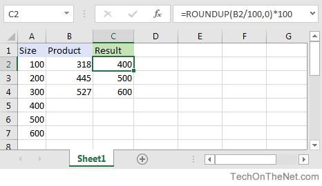
For example in cell C2, you can use the IF function and the ROUNDUP function as follows:

=ROUNDUP(B2/100,0)*100

This will return the correct value of 400 for a value of 318 in cell B2. Just copy this formula to cell C3, C4 and so on.

Источник

The IF function in Excel is used to give conditional outputs.

Syntax:

=IF(condition, value if TRUE, value if FALSE)

The IF statement in Excel checks the condition and returns the specified value if the condition is TRUE and another specified value if FALSE. At the place of value if TRUE and value of FALSE, you can put a value, a text within quotes, another formula or even another if statement (nested IF statement, we will talk about it).

Pro Note: IF in Excel 2016, 2013, and 2010 can have up to 64 nested IF statements. In Excel 2007 it was only 7.

The best thing about the IF statement is that you can customise TRUE and FALSE results. And this is what it is used for. Let’s see how…

IF Example 1:

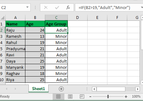
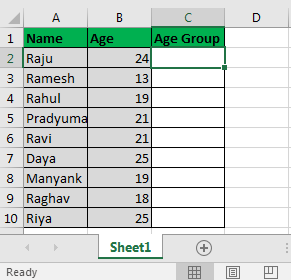
Assume you have a list of people. Now you want to know how many of them are adults and how many are minors.

Let’s say people whose age is greater than 19 are Adults and who are less than 19 are minor.

In Cell C2 write this excel IF statement and drag it down:

=IF(B2>19,»Adult»,»Minor»)

Here, Excel will simply check if the value in cell B2 is greater than 19 or not. Since it is greater than 19, it shows Adult in C2. And it does the same for all cells. Finally, we get this:

This was a simple example of an IF function in Excel. However, most of the time you would require nested IF or a combination of IF with other Excel functions.

Let’s have another example of the IF statement.

Example 2. Nested IF in Excel To Check Multiple Conditions

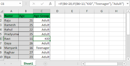
Assume, in a given list, you are required to tell if a kid is an Adult or “Teenager or KID”. And if Minor is then he is a teenager (between the age of 13 and 19) or a kid (below the age of 13).

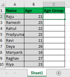
So here we have to do this

IF (is student’s age <20, if yes checkif(is student’s age <13, if yes then show “Kid”, If no then show “Teenager”), if No then show “Adult”)

There are other ways to do it but for the sake of understanding, we are taking this example.

Info: Most formulas are solved inside out but not IF statements. 
In a nested IF function, outer IF is solved first and then the inner IF. 
this is a basic diagram of the nested IFs control flow.

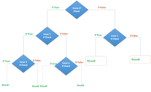
In cell C2, write this IF formula and drag it down to cell C10:

=IF(B6<20,IF(B6<13,»KID»,»Teenager»),»Adult»)

This is the final product we will have.

Now, let’s understand this. It’s easy.

IF(B6<20: this statement checks if the value in B6 is less than 20 not.

Since it is not, it skips the Value IF TRUE (IF(B6<13,»KID»,»Teenager»)) part and jumps to Value IF FALSE part and shows “Adult”.

Since most of them are above or equal to the age of 20, they are shown as “Adult”.

Note that Ravi is shown as “KID” as his age is 11 and Manyank is shown as “Teenager” as his age 16.

First, excel checks if Ravi’s age is <20. It’s TRUE. The control then moves to a TRUE section that contains another IF statement IF(B6<13. Next

Excel checks if Ravi<13. It’s TRUE. Control moves to the TRUE section of the IF. It contains “KID” and therefore it shows “KID” there.

Important Notes:

Nested IFs are solved inwards. The outer IF acts as a gateway to inner IF.
In Excel 2016, 2013 and 2010, you can have up to 64 steps of IF statements. In earlier Excel versions, it was only 7.
IF supports logical these operators = (equals to),< (less than), > (greater than) ,<= (less than or equal to),>= (greater than or equal to, <> (not equal to)
FALSE statements are optional, but TRUE options are mandatory.

Related Articles:

IF function with Wildcards

IF with OR Function in Excel

IF with AND Function in Excel

Popular Articles:

50 Excel Shortcut to Increase Your Productivity

How to use the VLOOKUP Function in Excel

How to use the COUNTIF function in Excel 2016

How to Use SUMIF Function in Excel

Источник

Значение, которое вы устанавливаете, когда два условия истинны или ложны.

Довольно часто количество возможных условий не 2 (проверенное и альтернативное), а 3, 4 и более. В этом случае вы также можете использовать функцию IF, но теперь вам придется поместить их одно в другое, указывая все условия по очереди. Рассмотрим следующий пример.

Несколько менеджеров по продажам должны получать премию в зависимости от выполнения плана продаж. Система поощрения выглядит следующим образом. Если план выполнен менее чем на 90%, премия не полагается, если от 90% до 95% — премия 10%, от 95% до 100% — премия 20%, а если план выполнен более чем достаточно — премия 30%. Как вы можете видеть, есть четыре варианта. Чтобы задать их в одной формуле, необходима следующая логическая структура. Если выполняется первое условие, то выполняется первый вариант, иначе, если выполняется второе условие, то выполняется второй вариант, иначе, если … и т.д. Количество условий может быть довольно большим. В конце формулы приводится последний альтернативный вариант, для которого не действует ни одно из вышеперечисленных условий (как третье поле в обычной формуле IF). В результате формула имеет следующий вид.

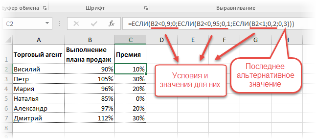
Комбинация функций IF работает таким образом, что если условие выполнено, то последующие условия больше не проверяются. Поэтому важно изложить их в правильном порядке. Если бы мы начали с B2

При написании формулы легко запутаться, поэтому стоит посмотреть на всплывающую подсказку.

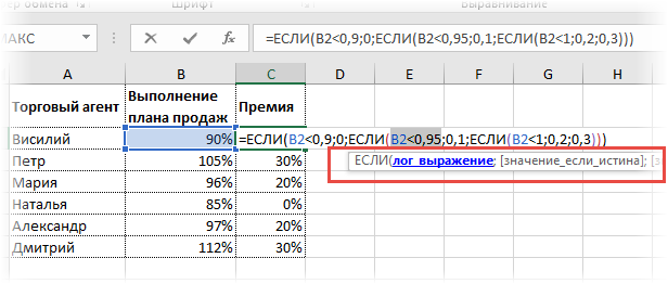
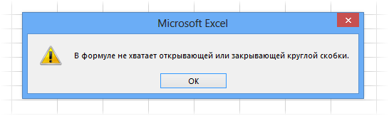
Не забудьте закрыть все круглые скобки в конце, иначе Excel выдаст ошибку

Синтаксис функции ЕСЛИ

Вот синтаксис и аргументы этой функции:

=If(булево выражение, значение, если «да», значение, если «нет»)

Логическое выражение — это (обязательное) условие, которое возвращает значение true или false («да» или «нет»);

Значение «да» — это (обязательное) действие, которое будет выполнено в случае положительного ответа;

Значение «нет» — это (обязательное) действие, предпринимаемое в случае отрицательного ответа;

Давайте рассмотрим эти аргументы вместе.

Первый аргумент — это логический вопрос. И этот ответ может быть только «да» или «нет», «истинным» или «ложным».

Как правильно задать вопрос? Вы можете построить логическое выражение, используя символы «=», «>», «=», «».

Расширение функционала с помощью операторов «И» и «ИЛИ»

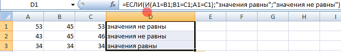
Когда необходимо проверить несколько истинных условий, используется функция AND, суть которой заключается в следующем: ЕСЛИ a = 1 И a = 2 ТО значение в ИЛИ равно c.

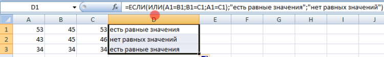
Функция ИЛИ проверяет, истинно ли условие 1 или условие 2. Если хотя бы одно условие истинно, результат будет истинным. Вывод таков: ЕСЛИ a = 1 ИЛИ a = 2 ТО значение в FATHER равно c.

Функции AND и OR могут проверять до 30 условий.

Пример использования оператора AND:

Пример использования функции ИЛИ:

Простейший пример применения.

Предположим, вы работаете в компании, которая продает шоколадные конфеты в нескольких регионах и обслуживает множество клиентов.

Мы должны отличать продажи, которые происходили в нашем регионе, от тех, которые были совершены за рубежом. Для этого нам нужно добавить в таблицу еще один атрибут для каждой продажи: страну, в которой она произошла. Мы хотим, чтобы этот атрибут создавался автоматически для каждой записи (т.е. строки).

В этом нам поможет функция IF. Добавим в таблицу данных столбец «Страна». Регион «Запад» — это местные продажи («Местные»), а остальные регионы — зарубежные продажи («Экспорт»).

Применение «ЕСЛИ» с несколькими условиями

Мы только что рассмотрели пример использования оператора «IF» с одним логическим выражением. Но вы также можете использовать более одного условия. Сначала будет проверена первая, и если она успешна, то значение будет выведено сразу. Только если первое логическое выражение не сработает, будет проверено второе.

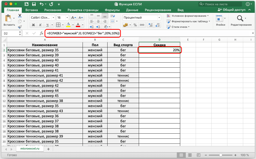
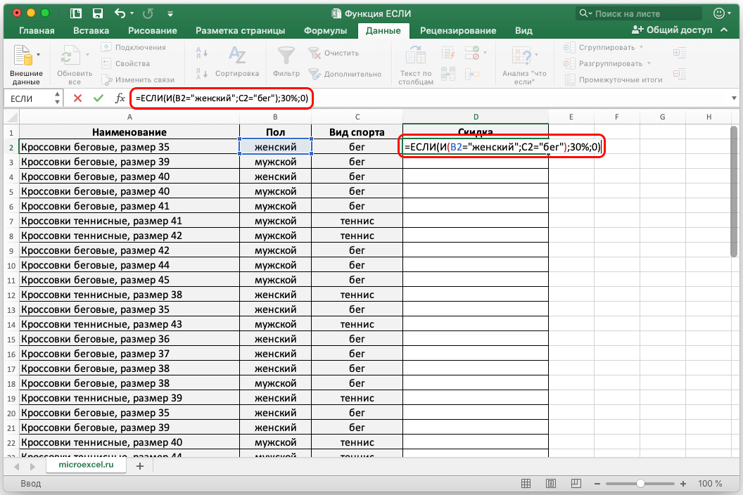
Рассмотрим пример той же таблицы. Но на этот раз давайте усложним задачу. Теперь нам нужно определить скидку на женскую обувь в зависимости от вида спорта.

Первое условие — проверка пола. Если это «мужчина» — сразу же отображается значение 0. Если это «женщина», то начинается вторая проверка условия. Если спорт — бег — 20%, если теннис — 10%.

Давайте напишем формулу для этих условий в нужной нам ячейке.

= IF(B2=»мужчина»;0; IF(C2=»бег»;20%;10%))

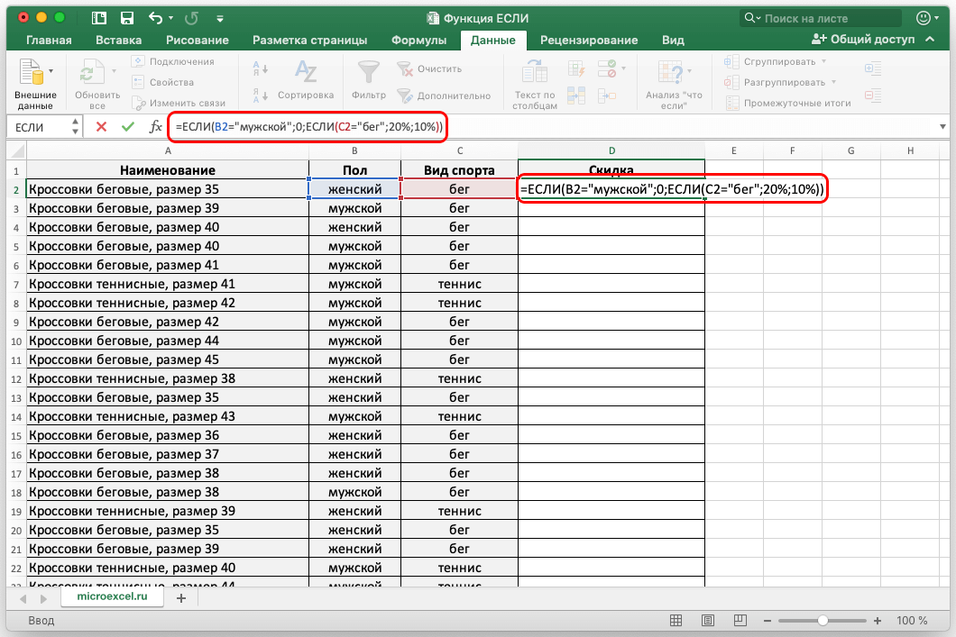
Нажимаем Enter и получаем результат в соответствии с заданными условиями.

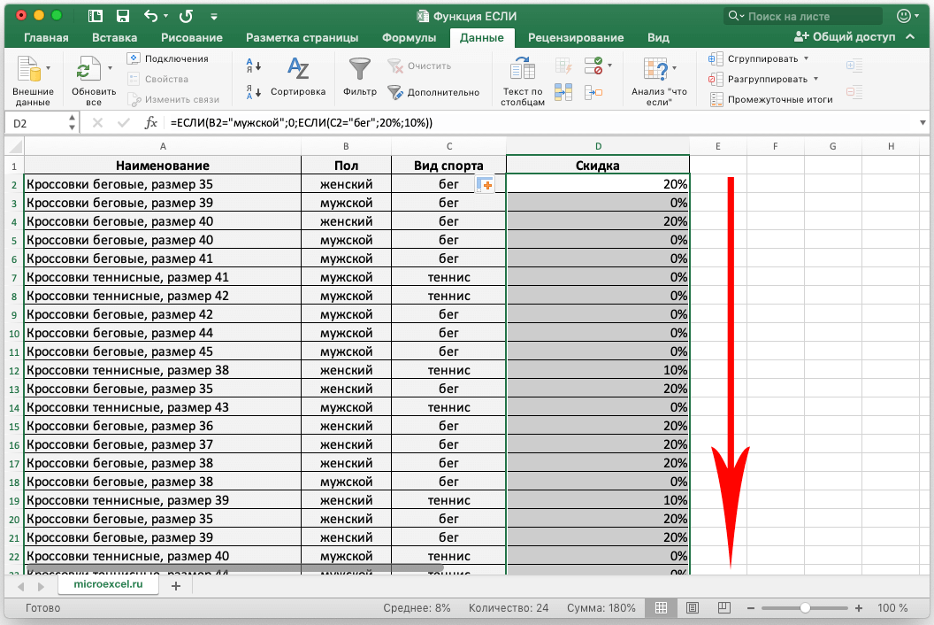
Затем распространите формулу на все остальные строки таблицы.

Операторы сравнения чисел и строк

Операторы, сравнивающие числа и строки, представлены операторами, состоящими из одного или двух математических знаков равенства и неравенства:

> — более чем;
>= — больше или равно;
= — равно;
— не равны.

Синтаксис:

1	Результат = Выражение1 Оператор Выражение2

Результат — любая числовая переменная;
Выражение — это выражение, которое возвращает число или строку;
Оператор — любой оператор, который сравнивает числа и строки.

Если переменная Result объявлена как Boolean (или Variant), она будет возвращать False и True. Числовые переменные других типов возвращают 0 (False) и -1 (True).

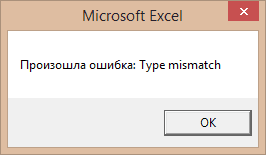
Операторы сравнения чисел и строк работают с двумя числами или двумя строками. При сравнении числа со строкой или строки с числом Excel VBA выдает ошибку несоответствия типов:

1 2 3 4 5 6 7 8 9 10

Sub Primer1() On Error GoTo Instr Dim myRes As Boolean ‘Сравнение строки с числом myRes = «пять» > 3 Instr: If Err.Description «» Then MsgBox «Произошла ошибка: » & Err.Description End If End Sub

Сравнение строк начинается с их первого символа. Если они равны, сравниваются следующие символы. И так далее, пока символы не станут разными, или одна или обе строки не закончатся.

Значения буквенных символов увеличиваются в алфавитном порядке, сначала все заглавные буквы, а затем все строчные. Если вы хотите сравнить длину строк, используйте функцию Len.

1 2 3

myRes = «семь» > «восемь» ‘myRes = True myRes = «семь» > «восемь» ‘myRes = False myRes = Len(«семь») > Len(«восемь») ‘myRes = False

Одновременное выполнение двух условий

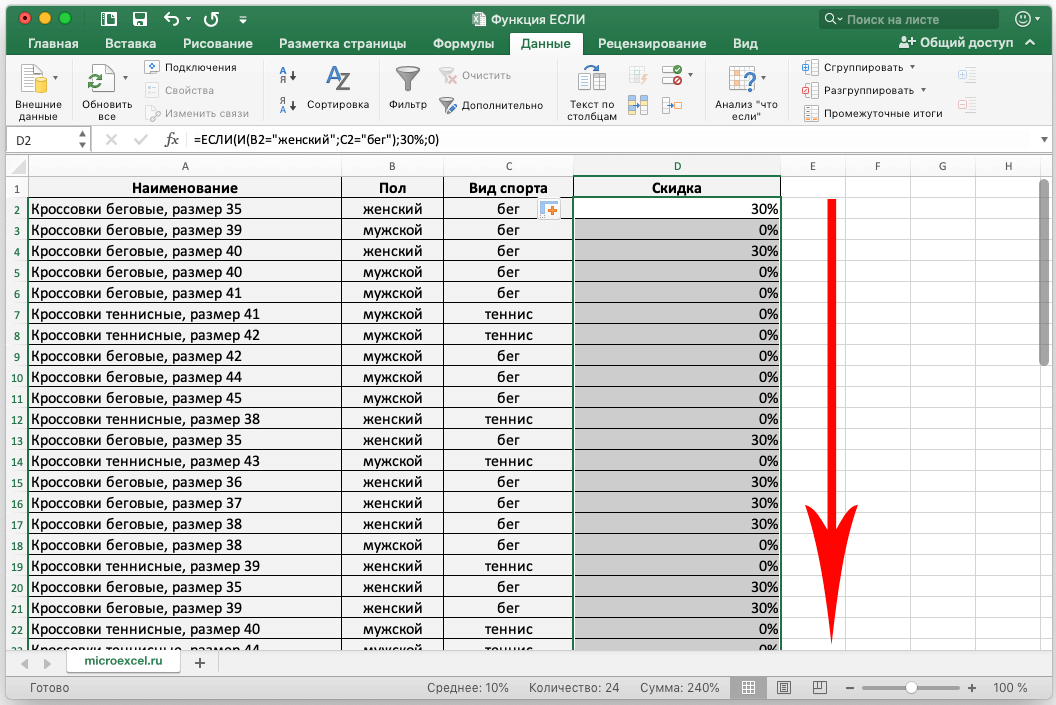
Также возможен вывод данных в Excel при одновременном выполнении двух условий. Таким образом, значение будет считаться ложным, если хотя бы одно из условий не выполняется. Для этого используется оператор «AND».

В качестве примера возьмем нашу таблицу. Теперь скидка в 30% будет предоставляться только в том случае, если это женская обувь, предназначенная для бега. Если эти условия выполняются одновременно, значение ячейки будет равно 30%, в противном случае оно будет равно 0.

Для этого используйте следующую формулу:

= IF(AND(B2=»women’s»;C2=»running»);30%;0)

Нажмите Enter, чтобы отобразить результат в ячейке.

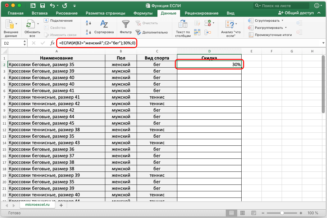
Как и в примерах выше, распространите формулу на оставшиеся строки.

Общее определение и задачи

«ЕСЛИ» — это стандартная функция Microsoft Excel. Его задача — проверить, выполняется ли определенное условие. Когда условие выполняется (true), оно возвращает одно значение в ячейке, где используется функция, а когда условие не выполняется (false), оно возвращает другое значение.

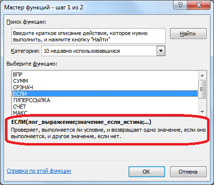
Синтаксис этой функции следующий: «IF(логическое выражение; [функция, если истинно]; [функция, если ложно])».

Как правильно записать?

Поместим курсор в ячейку G2 и введем знак «=». В Excel это означает, что теперь будет введена формула. Поэтому, как только вы нажмете «e», вам будет предложено выбрать функцию, начинающуюся на эту букву. Мы выбираем «ЕСЛИ».

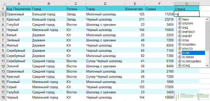
Все наши дальнейшие действия также будут подсказаны.

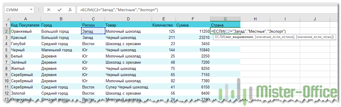
В качестве первого аргумента введите: C2=»Запад». Вам не нужно набирать адрес ячейки вручную, просто щелкните по ней мышью, как и в других функциях Excel. Затем вставьте «,» и укажите второй аргумент.

Второй аргумент — это значение, которое примет ячейка G2, если будет выполнено условие, которое мы записали. Это будет слово «Местный».

Затем мы снова указываем значение третьего аргумента, разделяя их запятыми. Это значение, которое примет ячейка G2, если условие не будет выполнено: «Экспорт». Не забудьте завершить ввод формулы, закрыв скобки и нажав клавишу «Enter».

Наша функция выглядит следующим образом:

= IF(C2=»Запад», «Местный», «Экспорт»)

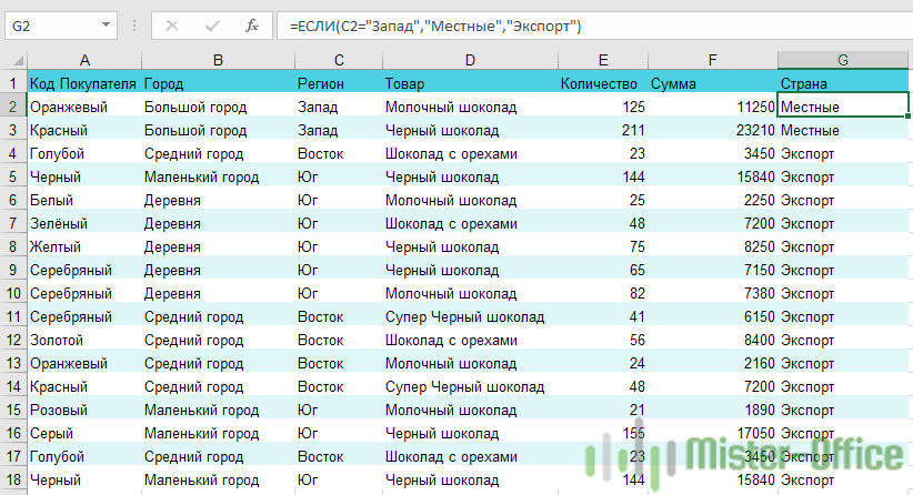
Наша ячейка G2 приняла значение «Местный».

Теперь нашу функцию можно скопировать во все остальные ячейки столбца G.

Дополнительная информация

Функция IF может одновременно тестировать 64 условия;
Если любой из аргументов функции является массивом — вычисляется каждый элемент массива;
Если в функции не указано условие для аргумента value_if_false, т.е. после аргумента value_if_false стоит только запятая (точка с запятой), то функция вернет «0», если результат функции FALSE.
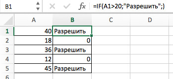
В примере ниже формула =IF(A1>20, «Разрешить») или =If(A1>20; «Разрешить»), где value_if_false не указано, но аргумент value_if_true по-прежнему следует через запятую. Функция возвращает «0» всякий раз, когда проверяемое условие не соответствует условию TRUE.

Если в функции не указано условие для аргумента TRUE(value_if_true), т.е. условие указано только для аргумента value_if_false, то формула будет возвращать «0» всякий раз, когда результатом вычисления функции будет TRUE;
В следующем примере формула имеет вид =IF(A1>20; «Запретить») или =If(A1>20; «Запретить»), где аргумент value_if_true не указан, формула будет возвращать «0» всякий раз, когда условие равно TRUE.

Вложенные условия с математическими выражениями.

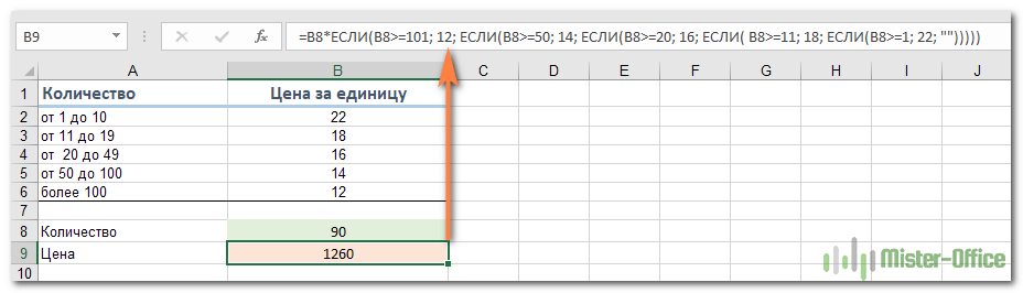
Вот еще одна типичная проблема: цена единицы товара варьируется в зависимости от его количества. Ваша цель — написать формулу, которая вычисляет цену для любого количества товара, введенного в данную ячейку. Другими словами, ваша формула должна проверять несколько условий и выполнять различные вычисления в зависимости от того, какой диапазон сумм содержит определенное количество товаров.

Эту задачу также можно выполнить с помощью нескольких вложенных функций ЕСЛИ. Логика такая же, как и в примере выше, за исключением того, что вы умножаете указанное количество на значение, возвращаемое вложенными условиями (т.е. соответствующую цену за единицу).

Если предположить, что количество хранится в B8, то формула будет выглядеть следующим образом:

=B8*IF(B8>=101; 12; IF(B8>=50; 14; IF(B8>=20; 16; IF( B8>=11; 18; IF(B8>=1; 22; «»)))))

И вот результат:

Как вы понимаете, этот пример демонстрирует лишь общий подход, и вы можете легко адаптировать эту вложенную функцию в зависимости от вашей конкретной задачи.

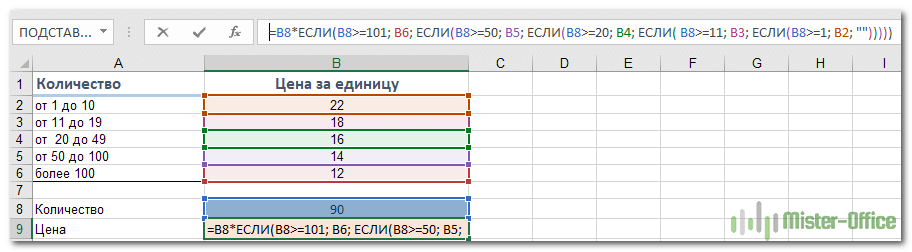
Например, вместо «жесткого» ввода цен в саму формулу можно обратиться к ячейкам, где они указаны (ячейки B2 — B6). Это позволит вам редактировать исходные данные без необходимости обновлять саму формулу:

=B8*IF(B8>=101; B6; IF(B8>=50; B5; IF(B8>=20; B4; IF( B8>=11; B3; IF(B8>=1; B2; «»)))))

Аргументы функции

logical_test (log_expression) — это условие, которое вы хотите проверить. Этот аргумент функции должен быть логическим и указываться как FALSE или TRUE. Аргументом может быть статическое значение или результат функции, вычисления;
[value_if_true] ([value_if_true]) — это (необязательное) значение, возвращаемое функцией. Он будет отображаться, если значение, которое мы проверяем, имеет условие TRUE;
[value_if_false] ([value_if_false]) — (необязательно) — это значение, которое возвращает функция. Он отобразится, если проверяемое условие соответствует условию FALSE.

А если один из параметров не заполнен?

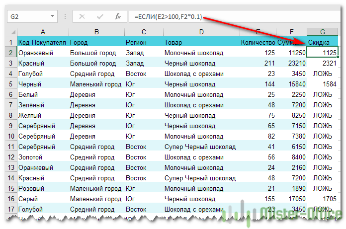
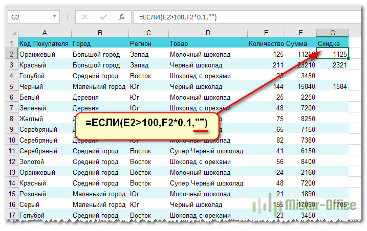
Если вас не интересует, что произойдет, например, если не будет выполнено интересующее вас условие, то вам не нужно приводить второй аргумент. Например, мы предоставляем скидку 10% при заказе более 100 штук. Мы не приводим никаких аргументов для случая, когда условие не выполняется.

=IF(E2>100,F2*0.1)

Каков будет результат этого?

Насколько это приятно и удобно — решать вам. Я считаю, что лучше использовать оба аргумента.

А если второе условие не выполняется, но вам ничего не нужно делать, вставьте в ячейку пустое значение.

=ЕСЛИ(E2>100,F2*0.1,””)

Однако эту конструкцию можно использовать в том случае, если значения «True» или «False» будут использоваться другими функциями Excel как булевы значения.

Обратите также внимание, что результирующие булевы значения в ячейке всегда центрируются. Это также можно увидеть на скриншоте выше.

Также, если вам действительно нужно просто проверить условие и получить «True» или «False» («Да» или «Нет»), вы можете использовать следующую конструкцию -…

=IF(E2>100,TRUE,FALSE)

Обратите внимание, что не обязательно использовать инвертированные запятые. Если вы поместите аргументы в инвертированные запятые, результатом функции IF будет текстовое, а не логическое значение.

Функция ЕПУСТО

Если вы хотите проверить, является ли ячейка пустой, вы можете использовать функцию EPUST (ISBLANK), которая имеет следующий синтаксис:

=EPUST(value)

Аргумент value может быть ссылкой на ячейку или диапазон. Если значение относится к пустой ячейке или диапазону, функция возвращает логическое значение TRUE, иначе FALSE.

Функции ИСТИНА и ЛОЖЬ

Функции TRUE и FALSE обеспечивают альтернативный способ записи логических значений TRUE и FALSE. Эти функции не имеют аргументов и выглядят следующим образом:

=TRUTH()
=FALSE().

Например, ячейка A1 содержит логическое выражение. Тогда следующая функция вернет «Pass», если выражение в ячейке A1 равно TRUE:

= IF(A1=ISTIN(); «Пройти»; «Остановиться»)

В противном случае формула вернет значение «Стоп».

Составное условие

Составное условие состоит из простых логических операций AND() и OR(), объединенных вместе.

AND() — это булева операция, которая требует одновременного выполнения всех связанных с ней условий.
OR() — это логическая операция, которая требует одновременного выполнения любого из связанных с ней условий.

Простое условие

Итак, что делает функция IF()? Посмотрите на диаграмму. Вот простой пример того, как эта функция работает для определения знака a.

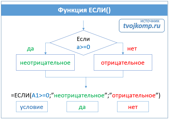
Блок-схема простого состояния. Определение отрицательных и неотрицательных чисел

Условие a>=0 определяет две возможности: неотрицательное число (нуль или положительное) и отрицательное число. Ниже приведено схематическое изображение формулы в Excel. За условием, за которым следует точка с запятой, следует список опций. Если условие истинно, в ячейке отобразится «неотрицательно», в противном случае — «отрицательно». Это запись, соответствующая ветви формулы «Да», за которой следует «Нет».

Текстовые данные в формуле заключаются в инвертированные запятые, а формулы и числа пишутся без инвертированных запятых.

Если результатом должен быть расчет, рассмотрите следующий пример. Давайте увеличим неотрицательное число на 10, а отрицательное оставим без изменений.

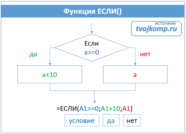
Простая диаграмма состояния. Расчет данных

На диаграмме видно, что если условие выполняется, то число увеличивается на десять, а вычисленное выражение A1+10 (выделено зеленым цветом) записывается в формулу Excel. В противном случае число не меняется, и вычисляемое выражение здесь состоит только из самого обозначения A1 (выделено красным цветом).

Это было краткое введение для новичков, которые только начинают изучать основы Excel. Теперь давайте рассмотрим более серьезный пример, в котором используется условная функция.

Задание:
Процентная ставка прогрессивного налога зависит от дохода. Если доход компании превышает определенную сумму, ставка налога выше. Используя функцию IF, рассчитайте сумму налога.

Решение:

Решение этой проблемы можно увидеть на рисунке ниже. Однако давайте поясним иллюстрацию. Основные исходные данные для решения этой задачи находятся в колонках A и B. В ячейке A5 показан предел дохода, при котором изменяется ставка налога. Соответствующие ставки указаны в ячейках B5 и B6. Доход компании указан в диапазоне ячеек B9:B14. Формула, которая рассчитывает налог, записана в ячейке C9: =If(B9>A$5;B9*B$6;B9*B$5). Эту формулу следует скопировать в ячейки ниже (выделены желтым цветом).

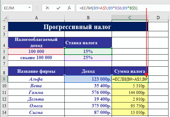
В формуле расчета адреса ячеек записаны как A$5, B$6, B$5. Знак доллара делает часть адреса, перед которой он ставится, постоянной при копировании формулы. Номер строки в адресе ячейки здесь не может изменяться.

Пример функции с несколькими условиями

В функции «ЕСЛИ» также можно ввести несколько условий. В этой ситуации инструкция «IF» вложена в другую. Если условие истинно, ячейка выводит набор результатов, но если условие не истинно, вывод зависит от второго оператора.

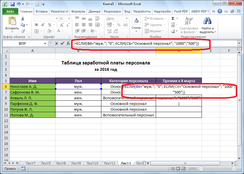
Как и в прошлый раз, «продлите» формулу вниз.

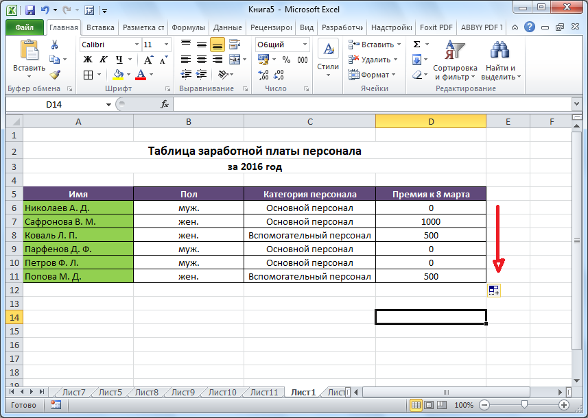
Пример использования «ЕСЛИ»

Теперь давайте рассмотрим конкретные примеры, где используется формула с оператором «IF».

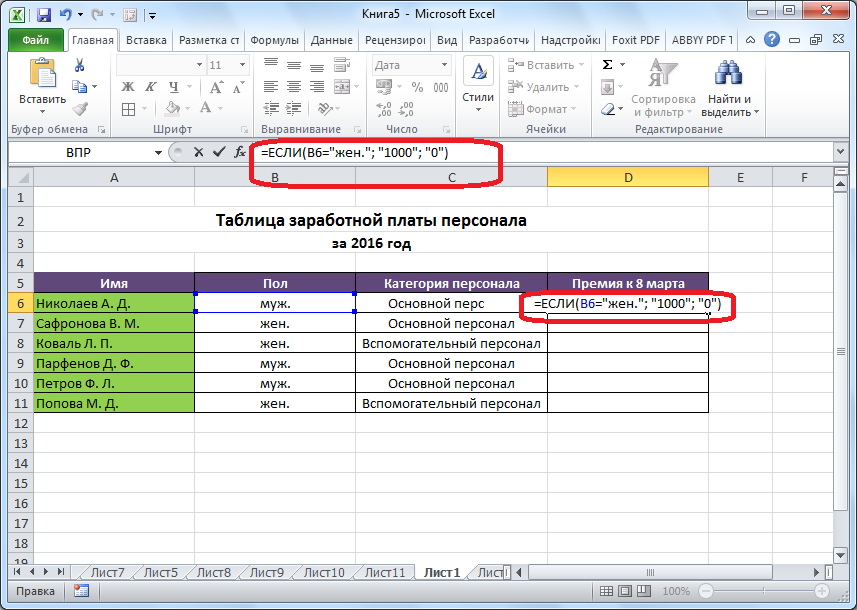
Затем нажмите клавишу Enter. Теперь, чтобы формула появилась в нижних ячейках, просто наведите курсор на правый нижний угол заполненной ячейки, нажмите левую кнопку мыши и, не отпуская ее, переместите курсор в нижнюю часть таблицы.

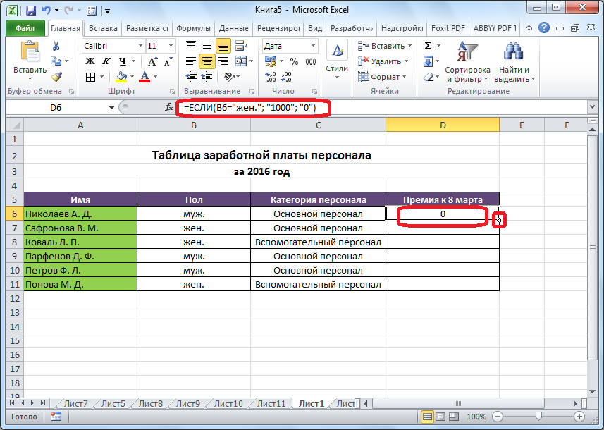
Таким образом, мы получили таблицу со столбцом, заполненным функцией «ЕСЛИ».

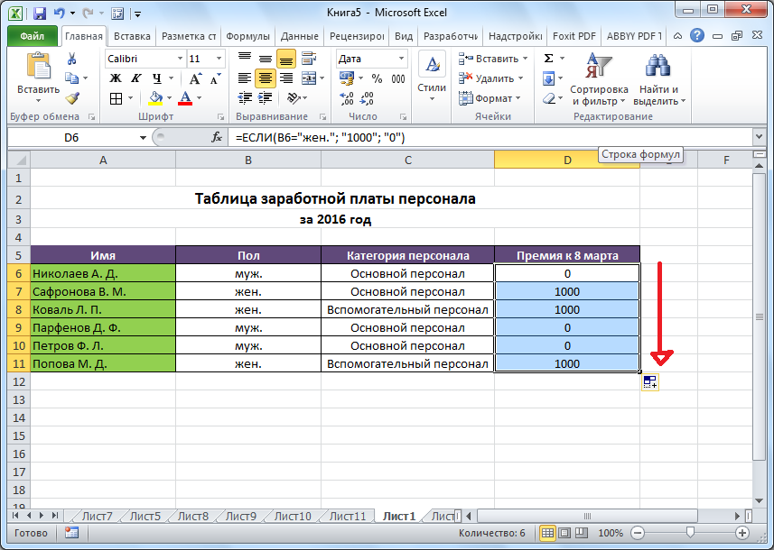
Проверяем простое числовое условие с помощью функции IF (ЕСЛИ)

При использовании функции ЕСЛИ в Excel можно применять различные операторы для проверки условия. Ниже приведен список операторов, которые вы можете использовать:

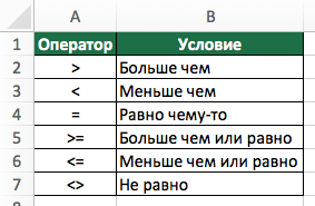
Если сумма баллов больше или равна «35», формула возвращает «Pass», в противном случае возвращает «Fail».

Заключение

Одним из самых популярных и полезных инструментов в Excel является функция IF, которая проверяет данные на соответствие заданным условиям и возвращает результат автоматически, исключая тем самым возможность человеческой ошибки. Поэтому знание и умение пользоваться этим инструментом сэкономит вам время не только на выполнение многих задач, но и на поиск возможных ошибок, возникающих при работе в «ручном» режиме.

Источник

The syntax of the IF() function is the following:

= IF ( logical_test , [value_if_TRUE] , [value_if_FALSE] )

The first two attributes are obligatory, i.e. without them, the formula doesn’t work, and produces an error message.

logical _test – a placeholder for the condition we want to test
value_if_TRUE – an attribute where we need to specify a value (text, or another function) that the IF formula returns when the result of the logical_test is TRUE

The third parameter is Optional, i.e. we can skip it and in such a case, the IF() function returns the default value FALSE.

value_if_FALSE – an attribute for a value, text or another formula that the IF() function must return when the result of the logical test is FALSE.

In other words, IF() function is used to test the specific conditions and can be described as the statement:

IF something is true, THEN return the first value, ELSE – return then second value.

The simplest IF() function may be written with the first two parameters only.

For example, this formula is absolutely correct:

 =IF(C2=1,"Hello!")

This formula tests the condition we set (C2=1) and if it is true, the formula returns the text message (“Hello!”).

Otherwise, it returns the default value FALSE.

Interesting Fact!!! You can use another simpler test in Excel for a certain condition. Just place a formula like “=C2>C3” in a cell and press ENTER. If this statement is true, the formula returns the default value – TRUE. Else (i.e. when a value in C2 is NOT larger than a value in C3 cell) the formula will return another default value – FALSE. We use the IF() function in these cases; when we want to trigger some further actions or calculations depending on the results of the logical test.

Typically, the IF() function is used in situations when we need to calculate or flag the results based on certain conditions (for example, smaller than, equal to, greater than and others).

Despite the fact that Excel usually provides multiple choices on how to solve every specific task, the IF() function can play a good role in such cases.

Another simple example of the IF() function:

=IF(C3="Hello!",1, 0)

If a value of the C3 cell is the text “Hello!” then this formula returns the one (1) value.

Else (i.e. if this cell contains any other text, number or blank value), the formula returns zero.

The big advantage of the IF() function (like many other Excel functions) is how we can replace all three arguments in this example with whatever we want/need and it still works properly (if we follow the syntax, of course).

For example, let’s replace the one (as a value_if_true) to another formula “C3+C4” and replace zero value (0) to TODAY() function.

Our initial formula becomes:

=IF(C3="Hello!",C2+C3,TODAY())

That means – IF a value in C2 cell equals one, THEN do the addition C2+C3.

ELSE (i.e. when C2 doesn’t equal “Hello!”), THEN execute the TODAY() function and return its result.

IF() function is a universal function, i.e. it accepts as an attribute different types of a value, such as numeric value, text, date/time, other functions, named ranges and others).

The IF function can be easily used as a part of other more complex formulas.

Moreover, you can use the so-called nested IF() function and replace the [value_if_false] with another IF() function.

The most common reason to do that is when you need to create a multi-choice comparison like a waterfall.

The last value_if_FALSE attribute is a value that we want the formula to return if the result of ALL logical tests in the formula is FALSE.

We know that we need to use a nested IF() (i.e. one IF() inside another IF() statement) when we have a “but” keyword inside the sentence with a logical test.

Take a look at the screenshot below.

In this example, we need to add the text “flag” if a value is greater than 200, BUT if this value is less than 50 we need to return “follow up” text.

We know that we need to use a nested IF() when there is the “but” keyword in the logical test.

Pro Tip: Be cautious. The more IF iterations we use, the more complex the formula becomes and the more difficult it is to understand. In addition, the complex formulas that contain multiple IF functions along with other Excel functions may slow down the calculation speed, especially if they use large ranges of cells. Also, it’s very easy to make an accidental mistake or typo inside the long and complex formulas, and such errors are difficult to trace properly.

The IF() function is often used with other logical functions such as AND() or OR() functions that we will discuss further.

Let’s look at some practical examples…

TEST CASE №1 Adding the word “Good” if the Revenue is greater than 15000

This is a typical use of the IF() function.

Let’s flag all apps if their Revenue is above 15,000.

Step 1. Go to the first cell where we need to insert a formula (cell C5 in this example).

Start the formula with an equal sign (=), add the keyword IF and the opened parentheses to make the formula look like:

=IF(

Step 2. The first argument of the IF() function is a logical test.

In this example, we want to flag a value in cell B5 (Revenue) if it is above 15000.

So, let’s continue the formula =IF(B5>15000,

Do not forget to put a comma once this step is ready.

This coma is used by Excel as a delimiter to separate the arguments from each other.

Pro tip: We can either type a numeric value in the logical test or use a cell reference to a cell that contains such a value (C2 cell in our example). The second approach is preferred because it gives us more flexibility in the future. Once we copy/paste the formula to the entire range, all we need to do in this case – if want to change that value – is go to the referral cell and change it there without needing to re-write the formula for all related cells.

NOTE: Keep in mind that if we want to use this approach, we need to fix the cell reference to look like $C$2. This fixed cell address is required for copying the formula to the entire range. Without that, the formula will return the wrong result. We can simply press F4 to fix the cell reference in the formula (make sure that the cursor is located near the appropriate cell address)

The formula becomes:

=IF(B5>$C$2,

Step 3. The second argument of IF() function, as we remember, is a value_if_TRUE.

Let’s type the text “Good” as a second attribute in the formula:

=IF(B5>$C$2, "Good",

Do not forget to put a comma once this step is ready.

Also, be careful – if you type a text value, you need to put it inside a double quotation mark (“your text”)

Pro tip: We can either type a numeric value in the logical test or use a cell reference to a cell that contains such a value (C3 cell in our example). If in the future we’ll decide to change the “Good” word to something else (“Not Bad”, for example), then all we need to do is go to cell C3 and change that text in the cell without the necessity to re-do the entire formula.

Our formula becomes:

=IF(B5>$C$2,$C$3,

NOTE: Don’t forget to fix the cell reference to look like $C$3 address. Press F4 to make an absolute reference. Without that, the formula will return a wrong result.

Step 4. The third argument of the IF() function is value_if_FALSE. We can skip this attribute (in such cases Excel returns the default value – FALSE). However, if we want to do that in a more aesthetic way, let the formula return a blank value. The blank value in Excel is equal to nothing between two quotation marks, like “”. So, the final version of the formula becomes:

=IF(B5>$C$2,$C$3,"")

NOTE: Don’t forget to close the brackets and press ENTER.

Step 5. Drag the formula down to the entire range.

Make a quick check manually to ensure that the formula returns the correct result according to our expectations.

TEST CASE №2 Adding the word “Good” if the Revenue is greater than 15000 and less than 20000

Let’s flag all apps if their Revenue is above 15,000 but under 20,000

Step 1. Go to the first cell where we need to insert a formula (cell D5 in this example).

Start the formula with an equal sign (=), add the keyword IF and the opened parentheses to make the formula look like:

=IF(

Step 2. The first argument of the IF() function is a logical test.

In this example, we want to flag a value in cell B5 (Revenue) if it is above 15000 and less than 20,000.

This is a typical situation when we can use the AND() logical function to unite several certain conditions into a single logical test.

AND() function can accept up to 255 conditions as its arguments.

Let’s continue the formula and add the second keyword AND with an opened parenthesis.

Once we’ve done that, we can type both conditions for the logical test inside AND() block and close its second parenthesis.

The formula looks like:

=IF(AND(B5>$D$2,B5<$D$3),

NOTE: Don’t forget to fix the cell reference to look like $D$2 and $D$3 address.

Press F4 to make an absolute reference.

Without that, the formula will return a wrong result after we drag it down to the entire range.

NOTE: Don’t forget to use a comma once this step is ready.

This comma is used by Excel as a delimiter to separate the arguments from each other.

Step 2. The second argument of IF() function, as we remember, is a value_if_TRUE.

Let’s add another cell reference as a second attribute in the formula:

=IF(AND(B5>$D$2,B5<$D$3),$C$3,

NOTE: Don’t forget to put a comma after the attribute once this step is ready. Be careful. If you type a text value, you need to put it inside a double quotation mark (“your text”)

Step 3. The third argument of the IF() function is a value_if_FALSE.

We can skip this attribute and Excel returns the default value – FALSE.

However, the more aesthetic way to do that is to return nothing (or blank value).

Nothing in Excel is denoted as a double quotation mark without any space:

=IF(AND(B5>$D$2,B5<$D$3),$C$3,"")

NOTE: Don’t forget to close the bracket and press ENTER.

Step 4. Drag the formula down to the entire range.

Make a quick check manually to ensure that the formula returns the correct result according to our expectations.

TEST CASE №3 Adding the word “Good” if the Revenue is greater than 15000 and less than 20000. Adding the word “Exceptional” if the Revenue is greater than or equal to 20,000. Otherwise, keeping the values

This time we’ll flag all apps as “Good” if their Revenue is above 15,000 and under 20,000.

In addition, we’ll flag them as “Exceptional” if their Revenue is greater than or equal to 20,000

Step 1. Go to the first cell where we need to insert a formula (cell E5 in this example).

Start the formula with an equal sign (=), add the keyword IF and the open parentheses to make the formula look like:

=IF(

Step 2. The first argument of the IF() function is a logical test.

The first part of the formula in this example is the same as we wrote in the previous example:

=IF(AND(B5>$E$2,B5<$E$3),$C$3,

NOTE: Don’t forget to to put a comma after the attribute once this step is ready.

Step 3. Usually, the third argument of the IF() function is a value_if_FALSE.

However, this time we need to add the second condition when a value in cell B5 is greater than or equal to 20,000.

We can do that if we use nested IF() function.

Let’s add another IF() block as a third parameter now:

=IF(AND(B5>$E$2,B5<$E$3),$C$3,IF(

Step 4. Add the second logical test, and the second value_if_TRUE.

In our example, the formula must return the “Exceptional” keyword if the value in cell B5 is greater than or equal to 20,000.

Let’s type this:

=IF(AND(B5>$E$2,B5<$E$3),$C$3,IF(B5>=$E$3,"Exceptional",

NOTE: If you type a value as a text, you need to put it inside a double quotation mark (“your text”)

Step 5. We need to write a value that the formula will return if the result of both logical tests is FALSE.

In our example, the formula must return the raw Revenue value in this case.

Let’s place this attribute as the third argument in the second IF() block:

=IF(AND(B5>$E$2,B5<$E$3),$C$3,IF(B5>=$E$3,"Exceptional",B5))

NOTE: Don’t forget to close the brackets.

We created two IF blocks, so we need to close two brackets at the end.

Step 6. Drag the formula down to the entire range.

Make a quick check manually to ensure that the formula returns the correct result according to our expectations.

TEST CASE №4 Adding the word “Flag” if the Revenue is greater than or equal to 20,000 OR it is lesser than or equal to 15,000

Let’s flag all apps if their Revenue is <= 15,000 or >= 20,000

Step 1. Go to the first cell where we need to insert a formula (cell D5 in this example).

Start the formula with an equal sign (=), add the keyword IF and the open parentheses to make the formula look like:

=IF(

Step 2. The first argument of the IF() function is a logical test.

In this example we want to flag a value in cell B5 (Revenue) if it is below or equal to 15000 OR above or equal to 20,000.

This is a situation when we can use OR() logical function that allows the testing of multiple logical conditions and return a true value if ANY of them is true.

Let’s continue the formula and add the second keyword OR with an opened bracket.

Once we’ve done that, we can type both conditions for the logical test inside OR() block and close its second parentheses.

The formula looks like:

=IF(OR(B5>=$F$2,B5=<$F$3),

NOTE: Press the F4 button on the keyboard to make an absolute reference.

Step 3. The second argument of the IF() function, as we remember, is a value_if_TRUE.

Let’s add this attribute in the formula:

=IF(AND(B5>$D$2,B5<$D$3),"Flag",

NOTE: If you type a text value, you need to put it inside a double quotation mark (“your text”)

Step 4. The third argument of the IF() function is a value_if_FALSE.

Let’s add a double quotation mark without any space to return a blank value:

=IF(AND(B5>$D$2, B5<$D$3),"Flag","")

NOTE: Don’t forget to close the bracket and press ENTER.

Step 5. Drag the formula down to the entire range.

Quickly check to ensure that the formula returns the correct result.

TEST CASE №5 Using other formulas inside the logical functions

Let’s calculate the difference between Actual Revenue and Budget Revenue and flag those cases when the difference is larger than +/- 10%.

Step 1. The easiest way to start building such a complex formula is to calculate the core value (this is the +/-10% threshold value in our case).

Step 2. Go to the first cell where we need to insert a formula (cell D23 in this example).

Start the formula with an equal sign (=), add the formula to calculate the difference (Actual divided by Budget minus one:

=B23/C23 - 1

Step 3. Let’s add the IF() block and the appropriate logical test.

This is a situation when we can use the OR() logical function as we need to flag a value if it is greater than +10% or lower than -10%:

=IF(OR(B23/C23 - 1>10%,B23/C23 - 1<-10%),

Step 4. The second argument of the IF() function, as we remember, is a value_if_TRUE.

In this example we need to return the exact deviation, so let’s do that, by simply copying the initial formula.

=IF(OR(B23/C23 - 1>10%,B23/C23 - 1<-10%),B23/C23 - 1,

Step 5. The third argument of the IF() function is a value_if_FALSE.

Let’s add a double quotation mark without any space to return a blank value:

=IF(OR(B23/C23 - 1>10%,B23/C23 - 1<-10%),B23/C23 - 1,"")

NOTE: Don’t forget to close the bracket and press ENTER.

Step 6. Drag the formula down to the entire range.

Quickly check to ensure that the formula returns the correct result.

TEST CASE №6 Using text symbols as the result of the IF() function

Let’s mark the positive deviation with the up arrow and the negative deviation with the down arrow.

Step 1. We’ll continue the previous example.

Let’s say we want to mark all positive deviations with a symbol that looks like an up arrow and all negative deviations with a symbol that looks like a down arrow.

First of all, a few preparations.

Let’s go to the cells above the test range (A20 and A21 cells in this example).

Feel free to select any other cells if you prefer.

Step 2. Insert the symbols that will indicate all positive and negative deviations.

To do this, we need to go on the INSERT tab on the Excel Ribbon and follow the path: INSERT > Symbol > Arial > Geometric Shapes

Click Insert once you have selected a shape.

Go to another cell below and insert the second arrow in the same way.

Step 3. Go to the first cell in the range where we want to add these visual indicators.

Replicate the IF() function with the cell references containing the arrows as the value_if_TRUE and value_if_FALSE attributes.

=IF(B23/C23 - 1>10%,$A$20,IF(B23/C23 - 1<-10%,$A$21,""))

NOTE: Don’t forget to close the bracket and press ENTER.

Step 4. Drag the formula down to the entire range.

Quickly check that the formula returns the correct result.

Workbook for Download

Feel free to Download the Workbook HERE.

Published on: February 1, 2018

Last modified: February 24, 2023

Leila Gharani

I’m a 5x Microsoft MVP with over 15 years of experience implementing and professionals on Management Information Systems of different sizes and nature.

My background is Masters in Economics, Economist, Consultant, Oracle HFM Accounting Systems Expert, SAP BW Project Manager. My passion is teaching, experimenting and sharing. I am also addicted to learning and enjoy taking online courses on a variety of topics.

Источник

Simple IF examples

Common problems

Need more help?

See Also

Need more help?

Want more options?

Что возвращает функция

Синтаксис

Аргументы функции

Дополнительная информация

Функция Если в Excel примеры с несколькими условиями

Пример 1. Проверяем простое числовое условие с помощью функции IF (ЕСЛИ)

Пример 2. Использование вложенной функции IF (ЕСЛИ) для проверки условия выражения

Пример 3. Вычисляем сумму комиссии с продаж с помощью функции IF (ЕСЛИ) в Excel

Пример 4. Используем логические операторы (AND/OR) (И/ИЛИ) в функции IF (ЕСЛИ) в Excel

Пример 5. Преобразуем ошибки в значения “0” с помощью функции IF (ЕСЛИ)

Syntax

Logical tests

Pass or Fail example

Assign points based on color

Return another formula

Nested IF statements

IF with AND, OR, NOT

IF cell contains specific text

More information

Notes

The syntax of the function «IF» with one condition

The function IF in Excel with multiple conditions

Enhanced functionality with the help of the operators «AND» and «OR»

How to compare data in two tables

How to Use the IF Function in Excel: Step-by-Step (2023)

How to use the IF function in Excel

IF and logical operators

Other IF formula examples

IF formula example #1

IF formula example #2

That’s it – Now what?

Frequently asked questions

Description

Syntax

Parameters or Arguments

Returns

Example (as Worksheet Function)

Combining the IF function with Other Logical Functions

AND function

OR function

Frequently Asked Questions

IF Example 1:

Example 2. Nested IF in Excel To Check Multiple Conditions

Синтаксис функции ЕСЛИ

Расширение функционала с помощью операторов «И» и «ИЛИ»

Простейший пример применения.

Применение «ЕСЛИ» с несколькими условиями

Операторы сравнения чисел и строк

Одновременное выполнение двух условий

Общее определение и задачи

Как правильно записать?

Дополнительная информация

Вложенные условия с математическими выражениями.

Аргументы функции

А если один из параметров не заполнен?

Функция ЕПУСТО

Функции ИСТИНА и ЛОЖЬ

Составное условие

Простое условие

Пример функции с несколькими условиями

Пример использования «ЕСЛИ»

Проверяем простое числовое условие с помощью функции IF (ЕСЛИ)

Заключение

TEST CASE №1 Adding the word “Good” if the Revenue is greater than 15000

TEST CASE №2 Adding the word “Good” if the Revenue is greater than 15000 and less than 20000

TEST CASE №3 Adding the word “Good” if the Revenue is greater than 15000 and less than 20000. Adding the word “Exceptional” if the Revenue is greater than or equal to 20,000. Otherwise, keeping the values

TEST CASE №4 Adding the word “Flag” if the Revenue is greater than or equal to 20,000 OR it is lesser than or equal to 15,000

TEST CASE №5 Using other formulas inside the logical functions

TEST CASE №6 Using text symbols as the result of the IF() function

Workbook for Download

Leila Gharani