
Excel for Microsoft 365 Excel 2021 Excel 2019 Excel 2016 Excel 2013 Excel 2010 Excel 2007 More…Less
Suppose you have a worksheet that contains confidential information, such as employee salaries, that you do not want a co-worker who stops by your desk to see. Or perhaps you multiply the values in a range of cells by the value in another cell that you do not want to be visible on the worksheet. By applying a custom number format, you can hide the values of those cells on the worksheet.
Note: Although cells with hidden values appear blank on the worksheet, their values remain displayed in the formula bar where you can work with them.
Hide cell values
-
Select the cell or range of cells that contains values that you want to hide. For more information, see Select cells, ranges, rows, or columns on a worksheet .
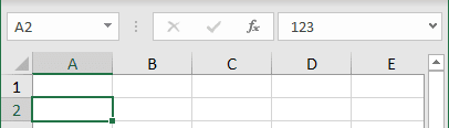
Note: The selected cells will appear blank on the worksheet, but a value appears in the formula bar when you click one of the cells.
-
On the Home tab, click the Dialog Box Launcher
 next to Number.
-
In the Category box, click Custom.
-
In the Type box, select the existing codes.
-
Type ;;; (three semicolons).
-
Click OK.
 next to Number.
Tip: To cancel a selection of cells, click any cell on the worksheet.
Display hidden cell values
-
Select the cell or range of cells that contains values that are hidden. For more information, see Select cells, ranges, rows, or columns on a worksheet .
-
On the Home tab, click the Dialog Box Launcher
next to Number.
-
In the Category box, click General to apply the default number format, or click the date, time, or number format that you want.
Tip: To cancel a selection of cells, click any cell on the worksheet.
Need more help?
Want more options?
Explore subscription benefits, browse training courses, learn how to secure your device, and more.
Communities help you ask and answer questions, give feedback, and hear from experts with rich knowledge.
Excel for Microsoft 365 for Mac Excel 2021 for Mac Excel 2019 for Mac Excel 2016 for Mac Excel for Mac 2011 More…Less
If you have a sheet that contains confidential information, such as employee salaries, you can hide the values of those cells by using a custom number format.
Do any of the following:
Hide cell values
When you hide a value in a cell, the cell appears to be empty. However, the formula bar still contains the value.
-
Select the cells.
-
On the Format menu, click Cells, and then click the Number tab.
-
Under Category, click Custom.
-
In the Type box, type ;;; (that is, three semicolons in a row), and then click OK.
Display hidden cell values
-
Select the cells.
-
On the Format menu, click Cells, and then click the Number tab.
-
Under Category, click General (or any appropriate date, time, or number format other than Custom), and then click OK.
See also
Protect workbooks or sheets (2016)
Protect a workbook
Protect a sheet (2011)
Need more help?
Want more options?
Explore subscription benefits, browse training courses, learn how to secure your device, and more.
Communities help you ask and answer questions, give feedback, and hear from experts with rich knowledge.
Содержание
- Display empty cells, null (#N/A) values, and hidden worksheet data in a chart
- Options for showing empty cells
- Options for cells with #N/A
- Change the way that empty cells, null (#N/A) values, and hidden rows and columns are displayed in a chart
- Need more help?
- Display or hide zero values
- How to hide the cell values in Excel without hiding cells
- Please, disable AdBlock and reload the page to continue
- Custom cell format
- Conditional formatting for chart axes
- How to hide points on the chart axis
By default, data that is hidden in rows and columns in the worksheet is not displayed in a chart, and empty cells or null values are displayed as gaps. For most chart types, you can display the hidden data in a chart.
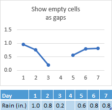
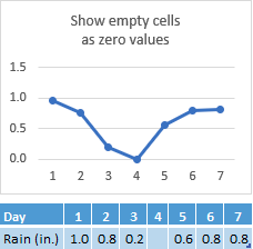
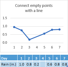
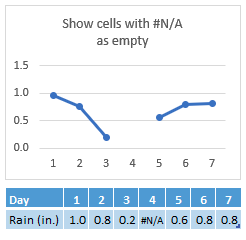
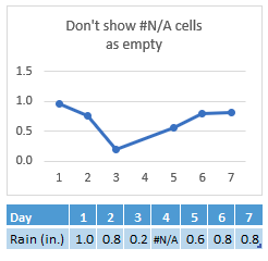
For line, scatter, and radar chart types, you can also change the way that empty cells, and cells that display the #N/A error are displayed in the chart. Instead of displaying empty cells as gaps, you can display empty cells as zero values (0), or you can span the gaps with a line. For #N/A values, you can choose to display those as an empty cell or connect data points with a line. The following examples show Excel’s behavior with each of these options.
Options for showing empty cells
Options for cells with #N/A
Change the way that empty cells, null (#N/A) values, and hidden rows and columns are displayed in a chart
Click the chart you want to change.
Go to Chart Tools on the Ribbon, then on the Design tab, in the Data group, click Select Data.
Click Hidden and Empty Cells.
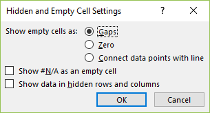
In the Show empty cells as: options box, click Gaps, Zero, or Connect data points with line.
Note: On a scatter chart that displays only markers (without connecting lines), you can display empty cells as gaps or zero only — you cannot connect the data points with a line.
Click the Show #N/A as an empty cell option if you don’t want Excel to plot those points.

This feature is only available if you have a Microsoft 365 subscription and is currently only available to Insiders. If you are a Microsoft 365 subscriber, make sure you have the latest version of Office.
In order to maintain backwards compatibility with other versions of Excel, this feature is off by default.
Click the Show data in hidden rows and columns option if you want Excel to plot hidden data.
Need more help?
You can always ask an expert in the Excel Tech Community, get support in the Answers community, or suggest a new feature or improvement. see How do I give feedback on Microsoft Office? to learn how to share your thoughts. We’re listening.
Источник
Display or hide zero values
You may have a personal preference to display zero values in a cell, or you may be using a spreadsheet that adheres to a set of format standards that requires you to hide zero values. There are several ways to display or hide zero values.
Sometimes you might not want zero (0) values showing on your worksheets, sometimes you need them to be seen. Whether your format standards or preferences call for zeroes showing or hidden, there are several ways to make it happen.
Hide or display all zero values on a worksheet
Click File > Options > Advanced.
Under Display options for this worksheet, select a worksheet, and then do one of the following:
To display zero (0) values in cells, check the Show a zero in cells that have zero value check box.
To display zero (0) values as blank cells, uncheck the Show a zero in cells that have zero value check box.
Hide zero values in selected cells
These steps hide zero values in selected cells by using a number format. The hidden values appear only in the formula bar and are not printed. If the value in one of these cells changes to a nonzero value, the value will be displayed in the cell, and the format of the value will be similar to the general number format.
Select the cells that contain the zero (0) values that you want to hide.
You can press Ctrl+1, or on the Home tab, click Format > Format Cells.
Click Number > Custom.
In the Type box, type 0;-0;;@, and then click OK.
To display hidden values:
Select the cells with hidden zeros.
You can press Ctrl+1, or on the Home tab, click Format > Format Cells.
Click Number > General to apply the default number format, and then click OK.
Hide zero values returned by a formula
Select the cell that contains the zero (0) value.
On the Home tab, click the arrow next to Conditional Formatting > Highlight Cells Rules Equal To.
In the box on the left, type 0.
In the box on the right, select Custom Format.
In the Format Cells box, click the Font tab.
In the Color box, select white, and then click OK.
Display zeros as blanks or dashes
Use the IF function to do this.
Use a formula like this to return a blank cell when the value is zero:
Here’s how to read the formula. If 0 is the result of (A2-A3), don’t display 0 – display nothing (indicated by double quotes “”). If that’s not true, display the result of A2-A3. If you don’t want the cells blank but want to display something other than 0, put a dash “-“ or other character between the double quotes.
Hide zero values in a PivotTable report
Click the PivotTable report.
On the Analyze tab, in the PivotTable group, click the arrow next to Options, and then click Options.
Click the Layout & Format tab, and then do one or more of the following:
Change error display Check the For error values show check box under Format. In the box, type the value that you want to display instead of errors. To display errors as blank cells, delete any characters in the box.
Change empty cell display Check the For empty cells show check box. In the box, type the value that you want to display in empty cells. To display blank cells, delete any characters in the box. To display zeros, clear the check box.
Sometimes you might not want zero (0) values showing on your worksheets, sometimes you need them to be seen. Whether your format standards or preferences call for zeroes showing or hidden, there are several ways to make it happen.
Display or hide all zero values on a worksheet
Click File > Options > Advanced.
Under Display options for this worksheet, select a worksheet, and then do one of the following:
To display zero (0) values in cells, select the Show a zero in cells that have zero value check box.
To display zero values as blank cells, clear the Show a zero in cells that have zero value check box.
Use a number format to hide zero values in selected cells
Follow this procedure to hide zero values in selected cells. If the value in one of these cells changes to a nonzero value, the format of the value will be similar to the general number format.
Select the cells that contain the zero (0) values that you want to hide.
You can use Ctrl+1, or on the Home tab, click Format > Format Cells.
In the Category list, click Custom.
In the Type box, type 0;-0;;@
The hidden values appear only in the formula bar — or in the cell if you edit within the cell — and are not printed.
To display hidden values again, select the cells, and then press Ctrl+1, or on the Home tab, in the Cells group, point to Format, and click Format Cells. In the Category list, click General to apply the default number format. To redisplay a date or a time, select the appropriate date or time format on the Number tab.
Use a conditional format to hide zero values returned by a formula
Select the cell that contains the zero (0) value.
On the Home tab, in the Styles group, click the arrow next to Conditional Formatting, point to Highlight Cells Rules, and then click Equal To.
In the box on the left, type 0.
In the box on the right, select Custom Format.
In the Format Cells dialog box, click the Font tab.
In the Color box, select white.
Use a formula to display zeros as blanks or dashes
To do this task, use the IF function.
The example may be easier to understand if you copy it to a blank worksheet.
Second number subtracted from the first (0)
Returns a blank cell when the value is zero (blank cell)
Returns a dash when the value is zero (-)
For more information about how to use this function, see IF function.
Hide zero values in a PivotTable report
Click the PivotTable report.
On the Options tab, in the PivotTable Options group, click the arrow next to Options, and then click Options.
Click the Layout & Format tab, and then do one or more of the following:
Change error display Select the For error values, show check box under Format. In the box, type the value that you want to display instead of errors. To display errors as blank cells, delete any characters in the box.
Change empty cell display Select the For empty cells, show check box. In the box, type the value that you want to display in empty cells. To display blank cells, delete any characters in the box. To display zeros, clear the check box.
Sometimes you might not want zero (0) values showing on your worksheets, sometimes you need them to be seen. Whether your format standards or preferences call for zeroes showing or hidden, there are several ways to make it happen.
Display or hide all zero values on a worksheet
Click the Microsoft Office Button  , click Excel Options, and then click the Advanced category.
Under Display options for this worksheet, select a worksheet, and then do one of the following:
To display zero (0) values in cells, select the Show a zero in cells that have zero value check box.
To display zero values as blank cells, clear the Show a zero in cells that have zero value check box.
Use a number format to hide zero values in selected cells
Follow this procedure to hide zero values in selected cells. If the value in one of these cells changes to a nonzero value, the format of the value will be similar to the general number format.
Select the cells that contain the zero (0) values that you want to hide.
You can press Ctrl+1, or on the Home tab, in the Cells group, click Format > Format Cells.
In the Category list, click Custom.
In the Type box, type 0;-0;;@
The hidden values appear only in the formula bar  — or in the cell if you edit within the cell — and are not printed.
To display hidden values again, select the cells, and then on the Home tab, in the Cells group, point to Format, and click Format Cells. In the Category list, click General to apply the default number format. To redisplay a date or a time, select the appropriate date or time format on the Number tab.
Use a conditional format to hide zero values returned by a formula
Select the cell that contains the zero (0) value.
On the Home tab, in the Styles group, click the arrow next to Conditional Formatting > Highlight Cells Rules > Equal To.
In the box on the left, type 0.
In the box on the right, select Custom Format.
In the Format Cells dialog box, click the Font tab.
In the Color box, select white.
Use a formula to display zeros as blanks or dashes
To do this task, use the IF function.
The example may be easier to understand if you copy it to a blank worksheet.
How do I copy an example?
Select the example in this article.
Important: Do not select the row or column headers.
Selecting an example from Help
In Excel, create a blank workbook or worksheet.
In the worksheet, select cell A1, and press CTRL+V.
Important: For the example to work properly, you must paste it into cell A1 of the worksheet.
To switch between viewing the results and viewing the formulas that return the results, press CTRL+` (grave accent), or on the Formulas tab > Formula Auditing group > Show Formulas.
After you copy the example to a blank worksheet, you can adapt it to suit your needs.
Источник
How to hide the cell values in Excel without hiding cells
1. Select cells which values you want to hide and do one of the following:
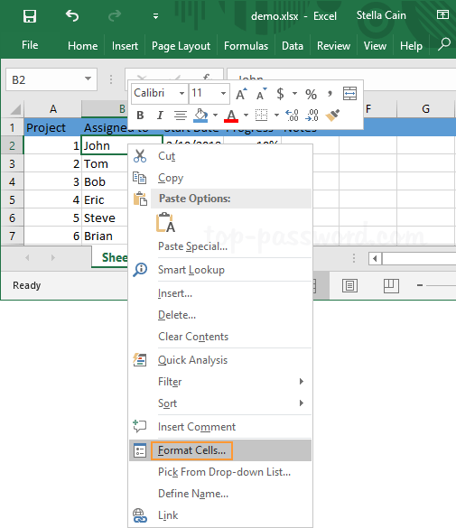
- Right-click on the selection and choose Format Cells. in the popup menu:
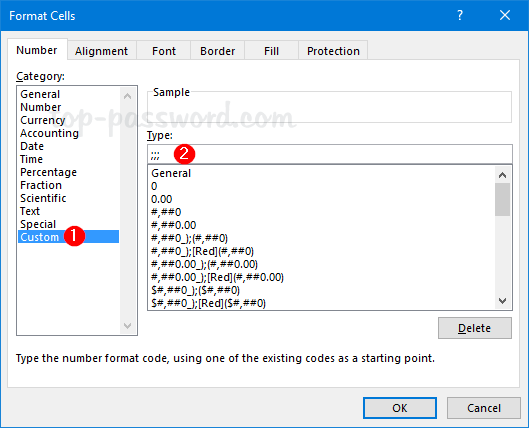
2. In the Format Cells dialog box, on the Number tab, select the Custom formatting, and then in the Type field, type «;;;» to hide any value in the cells:
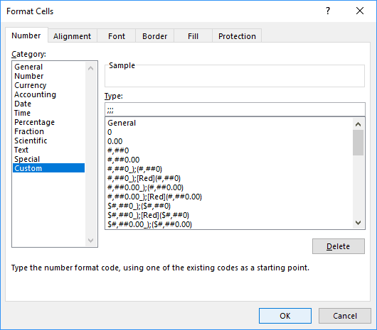
Note: The format code has four sections separated by semicolons:
Positive; Negative; Zero; Text
The empty sections mean no visible content to show.
See Custom cell format for more details.
Please, disable AdBlock and reload the page to continue
Today, 30% of our visitors use Ad-Block to block ads.We understand your pain with ads, but without ads, we won’t be able to provide you with free content soon. If you need our content for work or study, please support our efforts and disable AdBlock for our site. As you will see, we have a lot of helpful information to share.
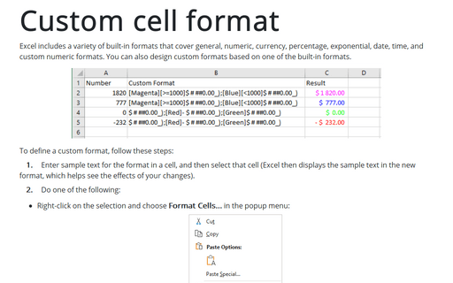
Custom cell format
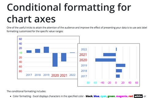
Conditional formatting for chart axes
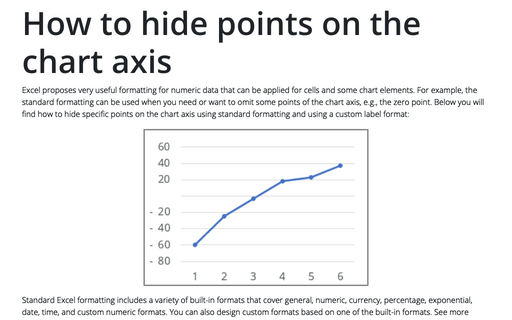
How to hide points on the chart axis
We use cookies to personalise content and ads, to provide social media features and to analyse our traffic. We also share information about your use of our site with our social media, advertising and analytics partners who may combine it with other information you’ve provided to them or they’ve collected from your use of their services.
Источник
Conditional formatting of Excel cells simplifies
highlighting values by adding color scales,
data bars, sparklines, and in-cell icons to the cell. The exact values of the highlighted cells
are rarely meaningful and may even interfere with the perception of information. Custom cell format
allows hiding values of such cells without hiding the cells.
1. Select cells which values you want to hide and do
one of the following:
- Right-click on the selection and choose Format Cells… in the popup menu:

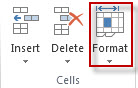
- On the Home tab, in the Number group, click the dialog box launcher:


2. In the Format Cells dialog box, on the Number
tab, select the Custom formatting, and then in the Type field, type «;;;»
to hide any value in the cells:
Note: The format code has four sections separated by semicolons:
Positive; Negative; Zero; Text
The empty sections mean no visible content to show.
See
Custom cell format for more details.
Please, disable AdBlock and reload the page to continue
Today, 30% of our visitors use Ad-Block to block ads.We understand your pain with ads, but without ads, we won’t be able to provide you with free content soon. If you need our content for work or study, please support our efforts and disable AdBlock for our site. As you will see, we have a lot of helpful information to share.
How can I hide the data in an individual cell I want to keep private? Hiding the confidential content of a cell is a useful trick most Excel users probably don’t know. In this tutorial we’ll walk you through the procedure to hide data or text in a cell in Excel 2016.
How to Hide Data or Text in an Excel Cell?
- Open your Excel spreadsheet in Excel 2016.
- Select the cells that contain sensitive data you want to hide. Right-click to choose “Format Cells” option from the drop-down menu.

- On the Number tab, choose the Custom category and enter three semicolons (;;;) without the parentheses into the Type box.

- Click OK and now the data in your selected cells is hidden.

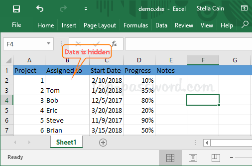
This method only hides the cell contents from being seen. The contents are still there and accessible for formulas, charts as such. If you want to display the hidden cell values, right-click the cells and select “Format Cells“. But this time choose “General” as the format of the cells.
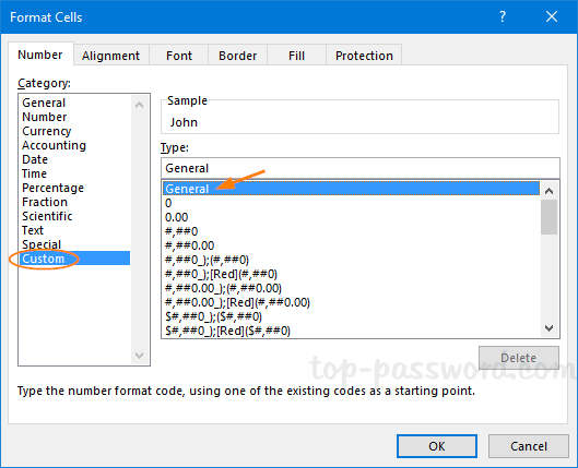
Now, the hidden text in your cells will be visible again.
- Previous Post: How to Hide / Unhide Entire Row or Column in Excel 2016
- Next Post: How to Change Text to Uppercase or Lowercase in Excel 2016
Working with large datasets that contain rows after rows of data can be quite painful.
In such cases, looking for data that match particular criteria can be like looking for a needle in a haystack.
Thankfully, Excel provides some features that let you hide certain rows based on the cell value so that you only see the rows that you want to see. There are two ways to do this:
- Using filters
- Using VBA
In this tutorial, we will discuss both methods, and you can pick the method you feel most comfortable with.
Using Filters to Hide Rows based on Cell Value
Let us say you have the dataset shown below, and you want to see data about only those employees who are still in service.

This is really easy to do using filters. Here are the steps you need to follow:
- Select the working area of your dataset.
- From the Data tab, select the Filter button. You will find it in the ‘Sort and Filter’ group.

- You should now see a small arrow button on every cell of the header row.

- These buttons are meant to help you filter your cells. You can click on any arrow to choose a filter for the corresponding column.
- In this example, we want to filter out the rows that contain the Employment status = “In service”. So, select the arrow next to the Employment Status header.
- Uncheck the boxes next to all the statuses, except “In service”. You can simply uncheck “Select All” to quickly uncheck everything and then just select “In service”.

- Click OK.


You should now be able to see only the rows with Employment Status=”In service”. All other rows should now be hidden.

Note: To unhide the hidden cells, simply click on the Filter button again.
Using VBA to Hide Rows based on Cell Value
The second method requires a little coding. If you are accustomed to using macros and a little coding using VBA, then you get much more scope and flexibility to manipulate your data to behave exactly the way you want.
Writing the VBA Code
The following code will help you display only the rows that contain information about employees who are ‘In service’ and will hide all other rows:
Sub HideRows()
StartRow = 2
EndRow = 19
ColNum = 3
For i = StartRow To EndRow
If Cells(i, ColNum).Value <> "In service" Then
Cells(i, ColNum).EntireRow.Hidden = True
Else
Cells(i, ColNum).EntireRow.Hidden = False
End If
Next i
End Sub
The macro loops through each cell of column C and hide the rows that do not contain the value “In service”. It should essentially analyze each cell from rows 2 to 19 and adjust the ‘Hidden’ attribute of the row that you want to hide.
To enter the above code, copy it and paste it into your developer window. Here’s how:
- From the Developer menu ribbon, select Visual Basic.

- Once your VBA window opens, you will see all your files and folders in the Project Explorer on the left side. If you don’t see Project Explorer, click on View->Project Explorer.

- Make sure ‘ThisWorkbook’ is selected under the VBA project with the same name as your Excel workbook.
- Click Insert->Module. You should see a new module window open up.

- Now you can start coding. Copy the above lines of code and paste them into the new module window.

- In our example, we want to hide the rows that do not contain the value ‘In service’ in column 3. But you can replace the value of ColNum number from “3” in line 4 to the column number containing your criteria values.
- Close the VBA window.


Note: If your dataset covers more than 19 rows, you can change the values of the StartRow and EndRow variables to your required row numbers.
If you can’t see the Developer ribbon, from the File menu, go to Options. Select Customize Ribbon and check the Developer option from Main Tabs.
Finally, Click OK.
Your macro is now ready to use.
Running the Macro
Whenever you need to use the above macro, all you need to do is run it, and here’s how:
- Select the Developer tab
- Click on the Macros button (under the Code group).
- This will open the Macro Window, where you will find the names of all the macros that you have created so far.
- Select the macro (or module) named ‘HideRows’ and click on the Run button.


You should see all the rows where Employment Status is not ’In service’ hidden.

Explanation of the Code
Here’s a line by line explanation of the above code:
- In line 1 we defined the function name.
Sub HideRows()
- In lines 2, 3 and 4 we defined variables to hold the starting row and ending row of the dataset as well as the index of the criteria column.
StartRow = 2
EndRow = 19
ColNum = 3
- In lines 5 to 11, we looped through each cell in column “3” (or column C) of the Active Worksheet. If a cell does not contain the value “Inservice”, then we set the ‘Hidden’ attribute of the entire row (corresponding to that cell) to True, which means we want to hide the entire corresponding row.
For i = StartRow To EndRow
If Cells(i, ColNum).Value <> "In service" Then
Cells(i, ColNum).EntireRow.Hidden = True
Else
Cells(i, ColNum).EntireRow.Hidden = False
End If
Next i
- Line 12 simply demarcates the end of the HideRows function.
End Sub
In this way, the above code hides all the rows that do not contain the value ‘In service’ in column C.
Un-hiding Columns Based On Cell Value
Now that we have been able to successfully hide unwanted rows, what if we want to see the hidden rows again?
Doing this is quite easy. You only need to make a small change to the HideRows function.
Sub UnhideRows()
StartRow = 2
EndRow = 19
ColNum = 3
For i = StartRow To EndRow
Cells(i, ColNum).EntireRow.Hidden = False
Next i
End Sub
Here, we simply ensured that irrespective of the value, all the rows are displayed (by setting the Hidden property of all rows to False).
You can run this macro in exactly the same way as HideRows.

Hiding Rows Based On Cell Values in Real-Time
In the first example, the columns are hidden only when the macro runs. However, most of the time, we want to hide columns on-the-fly, based on the value in a particular cell.
So, let’s now take a look at another example that demonstrates this. In this example, we have the following dataset:
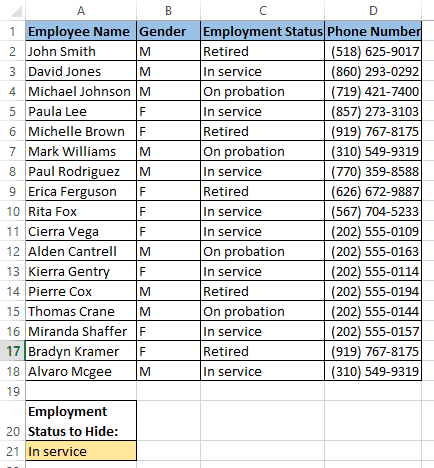
The only difference from the first dataset is that we have a value in cell A21 that will determine which rows should be hidden. So when cell A21 contains the value ‘Retired’ then only the rows containing the Employment Status ‘Retired’ are hidden.
Similarly, when cell A21 contains the value ‘On probation’ then only the rows containing the Employment Status ‘On probation’ are hidden.
When there is nothing in cell A21, we want all rows to be displayed.
We want this to happen in real-time, every time the value in cell A21 changes. For this, we need to make use of Excel’s Worksheet_SelectionChange function.
The Worksheet_SelectionChange Event
The Worksheet_SelectionChange procedure is an Excel built-in VBA event
It comes pre-installed with the worksheet and is called whenever a user selects a cell and then changes his/her selection to some other cell.
Since this function comes pre-installed with the worksheet, you need to place it in the code module of the correct sheet so that you can use it.
In our code, we are going to put all our lines inside this function, so that they get executed whenever the user changes the value in A21 and then selects some other cell.
Writing the VBA Code
Here’s the code that we are going to use:
StartRow = 2
EndRow = 19
ColNum = 3
For i = StartRow To EndRow
If Cells(i, ColNum).Value = Range("A21").Value Then
Cells(i, ColNum).EntireRow.Hidden = True
Else
Cells(i, ColNum).EntireRow.Hidden = False
End If
Next i
To enter the above code, you need to copy it and paste it in your developer window, inside your worksheet’s Worksheet_SelectionChange procedure. Here’s how:
- From the Developer menu ribbon, select Visual Basic.
- Once your VBA window opens, you will see all your project files and folders in the Project Explorer on the left side.
- In the Project Explorer, double click on the name of your worksheet, under the VBA project with the same name as your Excel workbook. In our example, we are working with Sheet1.
- This will open up a new module window for your selected sheet.
- Click on the dropdown arrow on the left of the window. You should see an option that says ‘Worksheet’.

- Click on the ‘Worksheet’ option. By default, you will see the Worksheet_SelectionChange procedure created for you in the module window.
- Now you can start coding. Copy the above lines of code and paste them into the Worksheet_SelectionChange procedure, right after the line: Private Sub Worksheet_SelectionChange(ByVal Target As Range).

- Close the VBA window.


Running the Macro
The Worksheet_SelectionChange procedure starts running as soon as you are done coding. So you don’t need to explicitly run the macro for it to start working.
Try typing the ‘Retired’ in the cell A21, then clicking any other cell. You should find all rows containing the value ‘Retired’ in column C disappear.

Now try replacing the value in cell A21 to ‘On probation’, then clicking any other cell. You should find all rows containing the value ‘On probation’ in column C disappear.

Now try removing the value in cell A21 and leaving it empty. Then click on any other cell. You should find both rows become visible again.

This means the code is working in real-time when changes are made to cell B20.
Explanation of the Code
Let us take a few minutes to understand this code now.
- Lines 1, 2, and 3 define variables to hold the starting row and ending row of the dataset as well as the index of the criteria column. You can change the values according to your requirement.
StartRow = 2
EndRow = 19
ColNum = 3
- Lines 4 to 10, loop through each cell in column “3” (or column C) of the worksheet. If the cell contains the value in cell A21, then we set the ‘Hidden’ attribute of the entire row (corresponding to that cell) to True, which means we want to hide the entire corresponding row.
For i = StartRow To EndRow
If Cells(i, ColNum).Value = Range("A21").Value Then
Cells(i, ColNum).EntireRow.Hidden = True
Else
Cells(i, ColNum).EntireRow.Hidden = False
End If
Next i
In this way, the above code hides the rows of the dataset depending on the value in cell A21. If A21 does not contain any value then the code displays all rows.
In this tutorial, I showed you how you can use Filters as well as Excel VBA to hide rows based on a cell value.
I did this with the help of two simple examples – one that removes required rows only when the macro is explicitly run and another that works in real-time.
I hope that we have been successful in helping you understand the concept behind the code so that you can customize it and use it in your own applications.
Other Excel tutorials you may also like:
- How to Hide Columns Based On Cell Value in Excel
- How to Delete Filtered Rows in Excel (with and without VBA)
- How to Highlight Every Other Row in Excel (Conditional Formatting & VBA)
- How to Unhide All Rows in Excel with VBA
- How to Set a Row to Print on Every Page in Excel
- How to Paste in a Filtered Column Skipping the Hidden Cells
- How to Select Multiple Rows in Excel
- How to Select Rows with Specific Text in Excel
- How to Move Row to Another Sheet Based On Cell Value in Excel?
- How to Compare Two Cells in Excel?
Imagine you’ve created a beautiful chart for your Excel report. You decide to hide the source data because the report’s users don’t need to see that. Suddenly the information in the chart disappears. So, this raises the question: how to show hidden data in an Excel chart?
We answer this question in this post. But, we go further. We also look at how we can use this technique for more advanced user interactivity.
Watch the video
Watch on YouTube
Download the example file
I recommend you download the example file for this post. Then you’ll be able to work along with examples and see the solution in action, plus the file will be helpful for future reference.
![]()
Download the file: 0113 Show hidden data in Excel chart.zip
The option to display or hide chart data is set on a chart-by-chart basis. It is one of those settings you have probably seen many times but never noticed it.
To show hidden data in an Excel chart:
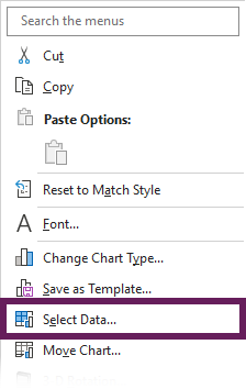
- Right-click on the chart. Click Select Data… from the menu.

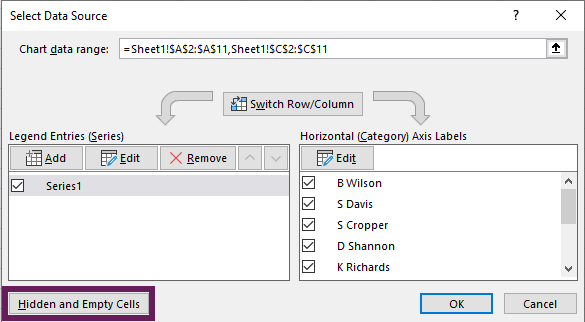
- In the Select Data Source dialog box, click the Hidden and Empty Cells button.

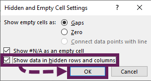
- The Hidden and Empty Cells Settings dialog box opens. Enable Show data in hidden rows and columns, then click OK.

- Click OK again to close the data source settings dialog box.
That’s it, that’s all it takes. The chart information is now visible again. Take a mental note of the additional settings in the Hidden and Empty Cells Settings dialog box; you never know when they might be useful.
Use hidden data to create dynamic charts
Initially, the feature to displaying hidden data may seem annoying. However, it actually creates a new level of flexibility for displaying charts. By combining this setting with AutoFilter, or an Excel Table, we can specify which rows to display inside a chart.
Example
The following is the source data for a chart:
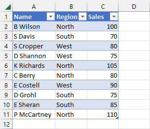
That source data as a bar chart displays as follows:
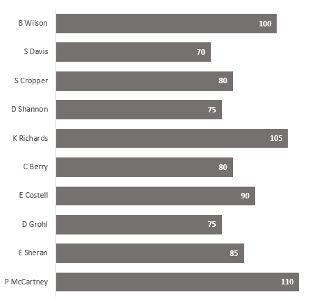
As the graph is connected to the Table, filtering the Table shows only the selected items in the chart.
As an example, I have selected North in the Region column of the Table. Therefore, the chart also updates displays only the North region.
This creates a flexible dashboard-style interactivity by harnessing the power of hidden rows.
VBA code to toggle between showing hidden/visible data
If we have a lot of charts, it can be time-consuming to apply this to each chart individually. The following VBA codes toggle the hidden cells setting in various scenarios.
For other VBA chart examples, check out this post: Ultimate Guide: VBA for Charts & Graphs in Excel (100+ examples)
Toggle hidden cells for active chart
The following code toggles the hidden cells setting on the active chart only.
Sub ToggleChartDisplayHiddenRows()

'Declare and assign variable
Dim cht As Chart
Set cht = ActiveChart

'Ignore errors if no chart active
On Error Resume Next

'Toggle hidden data visibility
cht.PlotVisibleOnly = Not cht.PlotVisibleOnly

On Error GoTo 0

End Sub
Toggle hidden cells for all charts on worksheet
The following code toggles the hidden cells for each chart.
Sub ToggleChartDisplayHiddenRowsAllOnSheet()

'Declare and assign variable
Dim chtObj As ChartObject

'Loop through all charts on the worksheet
For Each chtObj In ActiveSheet.ChartObjects

    'Toggle hidden data visibility
    chtObj.Chart.PlotVisibleOnly = Not chtObj.Chart.PlotVisibleOnly

Next

On Error GoTo 0

End Sub
Apply hidden setting of active chart to charts on same worksheet
The following code changes the setting for every chart on the worksheet to be identical to the active sheet.
Sub ToggleChartDisplayHiddenRowsSameAsActive()

'Declare and assign variable
Dim chtObj As ChartObject
Dim hiddenRowsSetting As Boolean

'Capture the PlotVisibility of active chart
hiddenRowsSetting = ActiveChart.PlotVisibleOnly

'Ignore errors if no chart active
On Error Resume Next

'Loop through all charts on the worksheet
For Each chtObj In ActiveSheet.ChartObjects

    'Toggle hidden data visibility
    chtObj.Chart.PlotVisibleOnly = hiddenRowsSetting

Next

On Error GoTo 0

End Sub
Office Scripts to toggle between showing hidden/visible data
Below are 3 Office Scripts that perform the same tasks as the VBA codes above.
Toggle hidden cells for active chart
The following script toggles the hidden cells setting on the active chart.
function main(workbook: ExcelScript.Workbook) {

//Declare and assign variable
let cht = workbook.getActiveChart()

//Ignore errors
try {
  //Toggle hidden data visibility
  cht.setPlotVisibleOnly(!cht.getPlotVisibleOnly())
} catch (err) {

}

}
Toggle hidden cells for all charts on worksheet
The following script toggles the hidden cells for every chart on the active worksheet.
function main(workbook: ExcelScript.Workbook) {

//Declare and assign variable
let ws = workbook.getActiveWorksheet()
let chtArr = ws.getCharts();

//Loop through all charts on the worksheet
for (let i = 0; i < chtArr.length; i++) {

  //Ignore errors
  try {
    //Toggle hidden data visibility
    chtArr[i].setPlotVisibleOnly(!chtArr[i].getPlotVisibleOnly())
  } catch (err) {

  }
}

}
Apply hidden setting of active chart to charts on same worksheet
The following script changes every chart on the worksheet to have the same setting as the active sheet.
function main(workbook: ExcelScript.Workbook) {

//Declare and assign variable
let ws = workbook.getActiveWorksheet()
let chtArr = ws.getCharts();

//Loop through all charts on the worksheet
for (let i = 0; i < chtArr.length; i++) {

  //Ignore errors
  try {
    //Toggle hidden data visibility
    chtArr[i].setPlotVisibleOnly(workbook.getActiveChart().getPlotVisibleOnly())
  } catch (err) {
  }
}

}
Conclusion
In this post, we have seen it is easy to show hidden data in an Excel chart. Then we saw how to harness the power of this feature to create dynamic charts which update based on filter selection. Finally, we looked at VBA and Office Scripts methods to automate changing the Show data in hidden rows and columns setting.

About the author
Hey, I’m Mark, and I run Excel Off The Grid.
My parents tell me that at the age of 7 I declared I was going to become a qualified accountant. I was either psychic or had no imagination, as that is exactly what happened. However, it wasn’t until I was 35 that my journey really began.
In 2015, I started a new job, for which I was regularly working after 10pm. As a result, I rarely saw my children during the week. So, I started searching for the secrets to automating Excel. I discovered that by building a small number of simple tools, I could combine them together in different ways to automate nearly all my regular tasks. This meant I could work less hours (and I got pay raises!). Today, I teach these techniques to other professionals in our training program so they too can spend less time at work (and more time with their children and doing the things they love).
Do you need help adapting this post to your needs?
I’m guessing the examples in this post don’t exactly match your situation. We all use Excel differently, so it’s impossible to write a post that will meet everybody’s needs. By taking the time to understand the techniques and principles in this post (and elsewhere on this site), you should be able to adapt it to your needs.
But, if you’re still struggling you should:
- Read other blogs, or watch YouTube videos on the same topic. You will benefit much more by discovering your own solutions.
- Ask the ‘Excel Ninja’ in your office. It’s amazing what things other people know.
- Ask a question in a forum like Mr Excel, or the Microsoft Answers Community. Remember, the people on these forums are generally giving their time for free. So take care to craft your question, make sure it’s clear and concise. List all the things you’ve tried, and provide screenshots, code segments and example workbooks.
- Use Excel Rescue, who are my consultancy partner. They help by providing solutions to smaller Excel problems.
What next?
Don’t go yet, there is plenty more to learn on Excel Off The Grid. Check out the latest posts:

This Excel tutorial explains how to unhide a value in a pivot table in Excel 2016 (with screenshots and step-by-step instructions).
If you want to follow along with this tutorial, download the example spreadsheet.
Download Example
Steps to Unhide a Value in a Pivot Table
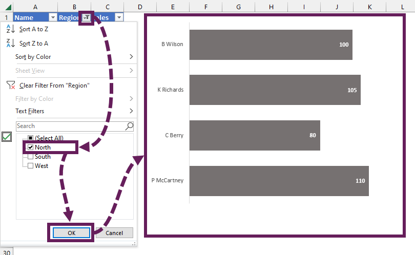
To show a hidden value in pivot table in Excel 2016, you will need to do the following steps:
-
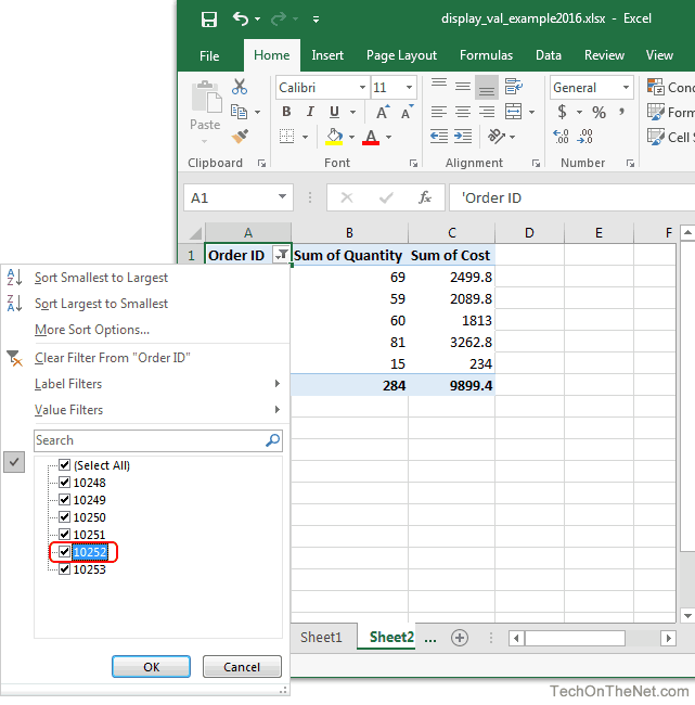
Look for the filter icon
 next to a pivot table heading. This indicates that a value has been hidden in the pivot table. In this example, Order #10252 has been hidden in the pivot table. We will show you how to unhide this value.
-
Click on the arrow to the right of the Order ID drop down box and select the checkbox for the 10252 value. Then click on the OK button.

TIP: All checked values are visible in the pivot table. All unchecked values are hidden in the pivot table.
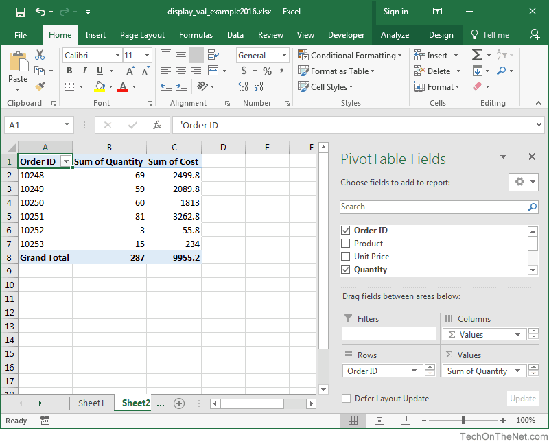
-
Now we can see the details for Order ID 10252 in the pivot table and the filter icon
is no longer next to the Order ID heading.
Как скрыть или отобразить строки и столбцы с помощью свойства Range.Hidden из кода VBA Excel? Примеры скрытия и отображения строк и столбцов.
Range.Hidden — это свойство, которое задает или возвращает логическое значение, указывающее на то, скрыты строки (столбцы) или нет.
Синтаксис
Expression — выражение (переменная), возвращающее объект Range.
- True — диапазон строк или столбцов скрыт;
- False — диапазон строк или столбцов не скрыт.
Примечание
Указанный диапазон (Expression) должен охватывать весь столбец или строку. Это условие распространяется и на группы столбцов и строк.
Свойство Range.Hidden предназначено для чтения и записи.
Примеры кода с Range.Hidden
Пример 1
Варианты скрытия и отображения третьей, пятой и седьмой строк с помощью свойства Range.Hidden:
|
Sub Primer1() ‘Скрытие 3 строки Rows(3).Hidden = True ‘Скрытие 5 строки Range(«D5»).EntireRow.Hidden = True ‘Скрытие 7 строки Cells(7, 250).EntireRow.Hidden = True MsgBox «3, 5 и 7 строки скрыты» ‘Отображение 3 строки Range(«L3»).EntireRow.Hidden = False ‘Скрытие 5 строки Cells(5, 250).EntireRow.Hidden = False ‘Скрытие 7 строки Rows(7).Hidden = False MsgBox «3, 5 и 7 строки отображены» End Sub |
Пример 2
Варианты скрытия и отображения третьего, пятого и седьмого столбцов из кода VBA Excel:
|
Sub Primer2() ‘Скрытие 3 столбца Columns(3).Hidden = True ‘Скрытие 5 столбца Range(«E2»).EntireColumn.Hidden = True ‘Скрытие 7 столбца Cells(25, 7).EntireColumn.Hidden = True MsgBox «3, 5 и 7 столбцы скрыты» ‘Отображение 3 столбца Range(«C10»).EntireColumn.Hidden = False ‘Отображение 5 столбца Cells(125, 5).EntireColumn.Hidden = False ‘Отображение 7 столбца Columns(«G»).Hidden = False MsgBox «3, 5 и 7 столбцы отображены» End Sub |
Пример 3
Варианты скрытия и отображения сразу нескольких строк с помощью свойства Range.Hidden:
|
1 2 3 4 5 6 7 8 9 10 11 12 13 14 15 16 17 |
Sub Primer3() ‘Скрытие одновременно 2, 3 и 4 строк Rows(«2:4»).Hidden = True MsgBox «2, 3 и 4 строки скрыты» ‘Скрытие одновременно 6, 7 и 8 строк Range(«C6:D8»).EntireRow.Hidden = True MsgBox «6, 7 и 8 строки скрыты» ‘Отображение 2, 3 и 4 строк Range(«D2:F4»).EntireRow.Hidden = False MsgBox «2, 3 и 4 строки отображены» ‘Отображение 6, 7 и 8 строк Rows(«6:8»).Hidden = False MsgBox «6, 7 и 8 строки отображены» End Sub |
Пример 4
Варианты скрытия и отображения сразу нескольких столбцов из кода VBA Excel:
|
1 2 3 4 5 6 7 8 9 10 11 12 13 14 15 16 17 |
Sub Primer4() ‘Скрытие одновременно 2, 3 и 4 столбцов Columns(«B:D»).Hidden = True MsgBox «2, 3 и 4 столбцы скрыты» ‘Скрытие одновременно 6, 7 и 8 столбцов Range(«F3:H40»).EntireColumn.Hidden = True MsgBox «6, 7 и 8 столбцы скрыты» ‘Отображение 2, 3 и 4 столбцов Range(«B6:D6»).EntireColumn.Hidden = False MsgBox «2, 3 и 4 столбцы отображены» ‘Отображение 6, 7 и 8 столбцов Columns(«F:H»).Hidden = False MsgBox «6, 7 и 8 столбцы отображены» End Sub |