
Excel for Microsoft 365 Excel for Microsoft 365 for Mac Excel for the web Excel 2021 Excel 2021 for Mac Excel 2019 Excel 2019 for Mac Excel 2016 Excel 2016 for Mac Excel 2013 Excel 2010 Excel 2007 Excel for Mac 2011 Excel Starter 2010 More…Less
This article describes the formula syntax and usage of the VALUE
function in Microsoft Excel.
Description
Converts a text string that represents a number to a number.
Syntax
VALUE(text)
The VALUE function syntax has the following arguments:
-
Text Required. The text enclosed in quotation marks or a reference to a cell containing the text you want to convert.
Remarks
-
Text can be in any of the constant number, date, or time formats recognized by Microsoft Excel. If text is not in one of these formats, VALUE returns the #VALUE! error value.
-
You do not generally need to use the VALUE function in a formula because Excel automatically converts text to numbers as necessary. This function is provided for compatibility with other spreadsheet programs.
Example
Copy the example data in the following table, and paste it in cell A1 of a new Excel worksheet. For formulas to show results, select them, press F2, and then press Enter. If you need to, you can adjust the column widths to see all the data.
|
Formula |
Description |
Result |
|---|---|---|
|
=VALUE(«$1,000») |
Number equivalent of the text string «$1,000» |
1000 |
|
=VALUE(«16:48:00»)-VALUE(«12:00:00») |
The serial number equivalent to 4 hours and 48 minutes, which is «16:48:00» minus «12:00:00» (0.2 = 4:48). |
0.2 |
Need more help?
Want more options?
Explore subscription benefits, browse training courses, learn how to secure your device, and more.
Communities help you ask and answer questions, give feedback, and hear from experts with rich knowledge.
Содержание
- Text functions (reference)
- Functions for working with text in Excel
- Examples with TEXT function in Excel
- Text splitting function in Excel
- Function for merging text in Excel
- Text SEARCH function in Excel
- VALUE Function
- Related functions
- Summary
- Purpose
- Return value
- Arguments
- Syntax
- Usage notes
- Dave Bruns
- Extract Numbers from a String in Excel (Using Formulas or VBA)
- Extract Numbers from String in Excel (Formula for Excel 2016)
- Extract Numbers from String in Excel (for Excel 2013/2010/2007)
- Separate Text and Numbers in Excel Using VBA
- Extract Numbers from String in Excel (using VBA)
- Extract Text from a String in Excel (using VBA)
Text functions (reference)
To get detailed information about a function, click its name in the first column.
Note: Version markers indicate the version of Excel a function was introduced. These functions aren’t available in earlier versions. For example, a version marker of 2013 indicates that this function is available in Excel 2013 and all later versions.
ARRAYTOTEXT function

Returns an array of text values from any specified range
Changes full-width (double-byte) English letters or katakana within a character string to half-width (single-byte) characters
Converts a number to text, using the ß (baht) currency format
Returns the character specified by the code number
Removes all nonprintable characters from text
Returns a numeric code for the first character in a text string
CONCAT function

Combines the text from multiple ranges and/or strings, but it doesn’t provide the delimiter or IgnoreEmpty arguments.
Joins several text items into one text item
DBCS function

Changes half-width (single-byte) English letters or katakana within a character string to full-width (double-byte) characters
Converts a number to text, using the $ (dollar) currency format
Checks to see if two text values are identical
Finds one text value within another (case-sensitive)
Formats a number as text with a fixed number of decimals
Returns the leftmost characters from a text value
Returns the number of characters in a text string
Converts text to lowercase
Returns a specific number of characters from a text string starting at the position you specify
NUMBERVALUE function
Converts text to number in a locale-independent manner
Extracts the phonetic (furigana) characters from a text string
Capitalizes the first letter in each word of a text value
Replaces characters within text
Repeats text a given number of times
Returns the rightmost characters from a text value
Finds one text value within another (not case-sensitive)
Substitutes new text for old text in a text string
Converts its arguments to text
Formats a number and converts it to text
TEXTAFTER function
Returns text that occurs after given character or string
TEXTBEFORE function
Returns text that occurs before a given character or string
TEXTJOIN function
Combines the text from multiple ranges and/or strings
TEXTSPLIT function
Splits text strings by using column and row delimiters
Removes spaces from text
UNICHAR function
Returns the Unicode character that is references by the given numeric value
UNICODE function
Returns the number (code point) that corresponds to the first character of the text
Converts text to uppercase
Converts a text argument to a number
VALUETOTEXT function
Returns text from any specified value
Important: The calculated results of formulas and some Excel worksheet functions may differ slightly between a Windows PC using x86 or x86-64 architecture and a Windows RT PC using ARM architecture. Learn more about the differences.
Источник
Functions for working with text in Excel
For the convenience of working with text in Excel, there are text functions. They make it easy to process hundreds of lines at once. Let’s consider some of them on examples.
Examples with TEXT function in Excel
This function converts numbers to string in Excel. Syntax: value (numeric or reference to a cell with a formula that gives a number as a result); Format (to display the number in the form of text).
The most useful feature of the TEXT function is the formatting of numeric data for merging with text data. Excel «doesn’t understand» how to display numbers without using the function. The program just converts them to a basic format.
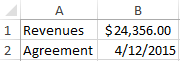
Let’s see an example. Let’s say you need to combine text in string with numeric values:
Using an ampersand without a function TEXT produces an inadequate result:
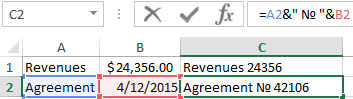
Excel returned the sequence number for the date and the general format instead of the monetary. The TEXT function is used to avoid this. It formats the values according to the user’s request.
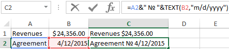
The formula «for a date» now looks like this:
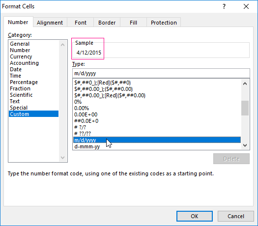
The second argument to the function is the format. Where to take the format line? Right-click on the cell with the value. Click on «Format Cells». In the opened window select «Custom». Copy the required «Type:» in the line. We paste the copied value in the formula.
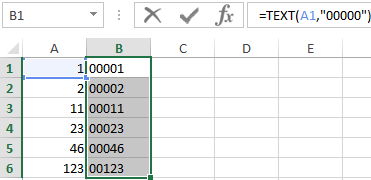
Let’s consider another example where this function can be useful. Add zeros at the beginning of the number. Excel will delete them if you enter it manually. Therefore, we introduce the formula:
If you want to return the old numeric values (without zeros), then use the «—» operator:
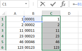
Note that the values are now displayed in numerical format.
Text splitting function in Excel
Individual functions and their combinations allow you to distribute words from one cell to separate cells:
- LEFT (Text, number of characters) displays the specified number of characters from the beginning of the cell;
- RIGHT (Text, number of characters) returns a specified number of characters from the end of the cell;
- SEARCH (Search text, range to search, start position) shows the position of the first occurrence of the searched character or line while viewing from left to right.
The line takes into account the position of each character when dividing the text. Spaces show the beginning or the end of the name you are looking for.
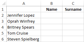
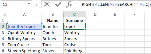
We will split the name, surname and patronymic name into different columns using the functions.
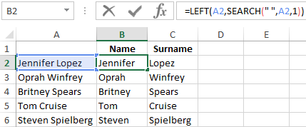
The first line contains only the first and last names separated by a space. Formula for retrieving the name:
The function SEARCH is used to determine the second argument of the LEFT function (the number of characters). It finds a space in cell A2 starting from the left.
For a name, we use the same formula:
Excel determines the number of characters for the RIGHT function using the SEARCH function. The LEN function «counts» the total length of the text. Then the number of characters up to the first space (found by SEARCH) is subtracted.
The formula for extracting the surname:
Next formulas for extracting the surname is a bit different:
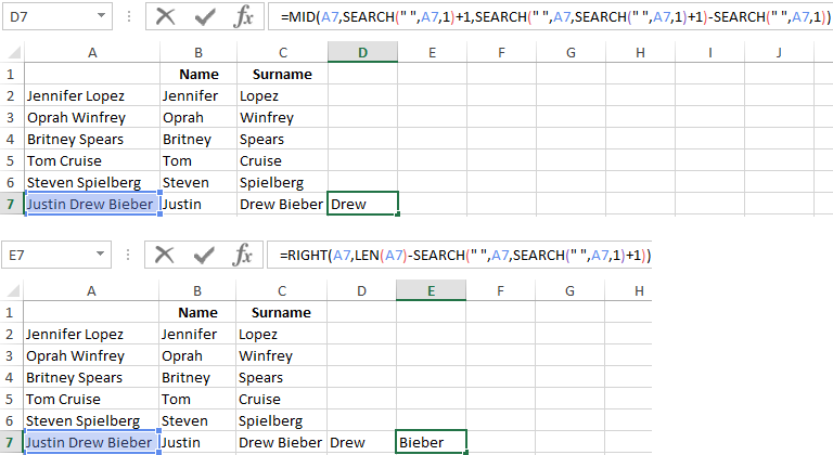
These are five signs on the right. Embedded SEARCH functions search for the second and third spaces in a string. SEARCH («»;A7;1) finds the first space on the left (before the patronymic name). Add one (+1) to the result. We get the position with which we will search for the second space.
Part of the formula SEARCH(» «;A7;SEARCH(» «;A7;1)+1) finds the second space. This will be the final position of the patronymic.
Then the number of characters from the beginning of the line to the second space is subtracted from the total length of the line. The result is the number of characters to the right that you need to return.
Function for merging text in Excel
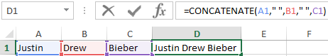
Use the ampersand (&) operator or the CONCATENATE function to combine values from several cells into one line.
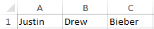
For example, the values are located in different columns (cells):
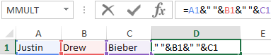
Put the cursor in the cell where the combined three values will be. Enter «=». Select the first cell and click on the keyboard «&» sign. Then enter the space character enclosed in quotation marks (» «). Enter again «&». Therefore, sequentially connect cells with symbols and spaces.
We get the combined values in one cell:
Using the CONCATENATE function:
You can add any sign or string to the final expression using quotation marks in the formula.
Text SEARCH function in Excel
The SEARCH function returns the starting position of the searched text (not case sensitive). For example:
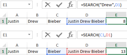
The SEARCH returned to position 8 because the word «Drew» begins with the tenth character in the line. Where can this be useful?
The SEARCH function determines the position of the character in the string line. And the MID function returns symbols values (see the example above). Alternatively, you can replace the found text with the REPLACE.
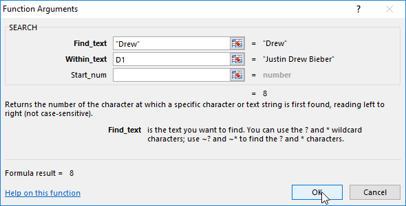
The syntax of the SEARCH function:
- «Find_text» is what you need to find;
- «Withing_text» is where to look;
- «Start_num» is from which position to start searching (by default it is 1).
Use the FIND if you need to take into account the case (lower and upper).
Источник
VALUE Function

Summary
The Excel VALUE function converts text that appears in a recognized format (i.e. a number, date, or time format) into a numeric value. Normally, the VALUE function is not needed in Excel, because Excel automatically converts text to numeric values.
Purpose
Return value
Arguments
- text — The text value to convert to a number.
Syntax
Usage notes
The VALUE function is meant to convert a text value that represents a number into a numeric value. The text can be a date, a time, or any other number, so long as the format can be recognized by Excel. When the conversion is successful, the result is a numeric value with no number formatting. When the VALUE function is unable to convert a text value to a numeric result, the result is a #VALUE! error.
In general, there is no need to use the VALUE function because Excel automatically converts text to numbers as needed. However, VALUE is provided for compatibility with other spreadsheet applications.
- Use the VALUE function to convert text input to a numeric value.
- The VALUE function converts text that appears in a recognized format (i.e. a number, date, or time format) into a numeric value.
- Normally, Excel automatically converts text to numeric values as needed, so the VALUE function is not needed.
- The VALUE function is provided for compatibility with other spreadsheet programs.
- The VALUE function returns #VALUE! when a conversion is unsuccessful.
Dave Bruns
Hi — I’m Dave Bruns, and I run Exceljet with my wife, Lisa. Our goal is to help you work faster in Excel. We create short videos, and clear examples of formulas, functions, pivot tables, conditional formatting, and charts.
Источник
Watch Video – How to Extract Numbers from text String in Excel (Using Formula and VBA)
There is no inbuilt function in Excel to extract the numbers from a string in a cell (or vice versa – remove the numeric part and extract the text part from an alphanumeric string).
However, this can be done using a cocktail of Excel functions or some simple VBA code.
Let me first show you what I am talking about.
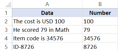
Suppose you have a data set as shown below and you want to extract the numbers from the string (as shown below):
The method you choose will also depend on the version of Excel you’re using:
- For versions prior to Excel 2016, you need to use slightly longer formulas
- For Excel 2016, you can use the newly introduced TEXTJOIN function
- VBA method can be used in all the versions of Excel
This Tutorial Covers:
This formula will work only in Excel 2016 as it uses the newly introduced TEXTJOIN function.
Also, this formula can extract the numbers that are at the beginning, end or middle of the text string.
Suppose you have the dataset as shown below and you want to extract the numbers from the strings in each cell:
Below is the formula that will give you numeric part from a string in Excel.
This is an array formula, so you need to use ‘Control + Shift + Enter‘ instead of using Enter.
In case there are no numbers in the text string, this formula would return a blank (empty string).
How does this formula work?
Let me break this formula and try and explain how it works:
- ROW(INDIRECT(“1:”&LEN(A2))) – this part of the formula would give a series of numbers starting from one. The LEN function in the formula returns the total number of characters in the string. In the case of “The cost is USD 100”, it will return 19. The formulas would thus become ROW(INDIRECT(“1:19”). The ROW function will then return a series of numbers –
- (MID(A2,ROW(INDIRECT(“1:”&LEN(A2))),1)*1) – This part of the formula would return an array of #VALUE! errors or numbers based on the string. All the text characters in the string become #VALUE! errors and all numerical values stay as-is. This happens as we have multiplied the MID function with 1.
- IFERROR((MID(A2,ROW(INDIRECT(“1:”&LEN(A2))),1)*1),””) – When IFERROR function is used, it would remove all the #VALUE! errors and only the numbers would remain. The output of this part would look like this –
- =TEXTJOIN(“”,TRUE,IFERROR((MID(A2,ROW(INDIRECT(“1:”&LEN(A2))),1)*1),””)) – The TEXTJOIN function now simply combines the string characters that remains (which are the numbers only) and ignores the empty string.
Download the Example File 
You can also use the same logic to extract the text part from an alphanumeric string. Below is the formula that would get the text part from the string:
A minor change in this formula is that IF function is used to check if the array we get from MID function are errors or not. If it’s an error, it keeps the value else it replaces it with a blank.
Then TEXTJOIN is used to combine all the text characters.
If you have Excel 2013. 2010. or 2007, you can not use the TEXTJOIN formula, so you will have to use a complicated formula to get this done.
Suppose you have a dataset as shown below and you want to extract all the numbers in the string in each cell.
The below formula will get this done:
In case there is no number in the text string, this formula would return blank (empty string).
Although this is an array formula, you don’t need to use ‘Control-Shift-Enter’ to use this. A simple enter works for this formula.
Credit to this formula goes to the amazing Mr. Excel forum.
Again, this formula will extract all the numbers in the string no matter the position. For example, if the text is “The price of 10 tickets is USD 200”, it will give you 10200 as the result.
Separate Text and Numbers in Excel Using VBA
If separating text and numbers (or extracting numbers from the text) is something you have to often, you can also use the VBA method.
All you need to do is use a simple VBA code to create a custom User Defined Function (UDF) in Excel, and then instead of using long and complicated formulas, use that VBA formula.
Let me show you how to create two formulas in VBA – one to extract numbers and one to extract text from a string.
In this part, I will show you how to create the custom function to get only the numeric part from a string.
Below is the VBA code we will use to create this custom function:
Here are the steps to create this function and then use it in the worksheet:
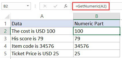
Now, you will be able to use the GetText function in the worksheet. Since we have done all the heavy lifting in the code itself, all you need to do is use the formula =GetNumeric(A2).
This will instantly give you only the numeric part of the string.
Note that since the workbook now has VBA code in it, you need to save it with .xls or .xlsm extension.
Download the Example File
In case you have to use this formula often, you can also save this to your Personal Macro Workbook. This will allow you to use this custom formula in any of the Excel workbooks that you work with.
In this part, I will show you how to create the custom function to get only the text part from a string.
Below is the VBA code we will use to create this custom function:
Here are the steps to create this function and then use it in the worksheet:
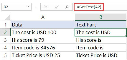
Now, you will be able to use the GetNumeric function in the worksheet. Since we have done all the heavy lifting in the code itself, all you need to do is use the formula =GetText(A2) .
This will instantly give you only the numeric part of the string.
Note that since the workbook now has VBA code in it, you need to save it with .xls or .xlsm extension.
In case you have to use this formula often, you can also save this to your Personal Macro Workbook. This will allow you to use this custom formula in any of the Excel workbooks that you work with.
In case you’re using Excel 2013 or prior versions and don’t have
You May Also Like the Following Excel Tutorials:
Источник
For the convenience of working with text in Excel, there are text functions. They make it easy to process hundreds of lines at once. Let’s consider some of them on examples.
Examples with TEXT function in Excel
This function converts numbers to string in Excel. Syntax: value (numeric or reference to a cell with a formula that gives a number as a result); Format (to display the number in the form of text).
The most useful feature of the TEXT function is the formatting of numeric data for merging with text data. Excel «doesn’t understand» how to display numbers without using the function. The program just converts them to a basic format.
Let’s see an example. Let’s say you need to combine text in string with numeric values:
Using an ampersand without a function TEXT produces an inadequate result:
Excel returned the sequence number for the date and the general format instead of the monetary. The TEXT function is used to avoid this. It formats the values according to the user’s request.
The formula «for a date» now looks like this:
The second argument to the function is the format. Where to take the format line? Right-click on the cell with the value. Click on «Format Cells». In the opened window select «Custom». Copy the required «Type:» in the line. We paste the copied value in the formula.
Let’s consider another example where this function can be useful. Add zeros at the beginning of the number. Excel will delete them if you enter it manually. Therefore, we introduce the formula:
If you want to return the old numeric values (without zeros), then use the «—» operator:
Note that the values are now displayed in numerical format.
Text splitting function in Excel
Individual functions and their combinations allow you to distribute words from one cell to separate cells:
- LEFT (Text, number of characters) displays the specified number of characters from the beginning of the cell;
- RIGHT (Text, number of characters) returns a specified number of characters from the end of the cell;
- SEARCH (Search text, range to search, start position) shows the position of the first occurrence of the searched character or line while viewing from left to right.
The line takes into account the position of each character when dividing the text. Spaces show the beginning or the end of the name you are looking for.
We will split the name, surname and patronymic name into different columns using the functions.
The first line contains only the first and last names separated by a space. Formula for retrieving the name:
The function SEARCH is used to determine the second argument of the LEFT function (the number of characters). It finds a space in cell A2 starting from the left.
For a name, we use the same formula:
Excel determines the number of characters for the RIGHT function using the SEARCH function. The LEN function «counts» the total length of the text. Then the number of characters up to the first space (found by SEARCH) is subtracted.
The formula for extracting the surname:
Next formulas for extracting the surname is a bit different:
These are five signs on the right. Embedded SEARCH functions search for the second and third spaces in a string. SEARCH («»;A7;1) finds the first space on the left (before the patronymic name). Add one (+1) to the result. We get the position with which we will search for the second space.
Part of the formula SEARCH(» «;A7;SEARCH(» «;A7;1)+1) finds the second space. This will be the final position of the patronymic.
Then the number of characters from the beginning of the line to the second space is subtracted from the total length of the line. The result is the number of characters to the right that you need to return.
Function for merging text in Excel
Use the ampersand (&) operator or the CONCATENATE function to combine values from several cells into one line.
For example, the values are located in different columns (cells):
Put the cursor in the cell where the combined three values will be. Enter «=». Select the first cell and click on the keyboard «&» sign. Then enter the space character enclosed in quotation marks (» «). Enter again «&». Therefore, sequentially connect cells with symbols and spaces.
We get the combined values in one cell:
Using the CONCATENATE function:
You can add any sign or string to the final expression using quotation marks in the formula.
Text SEARCH function in Excel
The SEARCH function returns the starting position of the searched text (not case sensitive). For example:
The SEARCH returned to position 8 because the word «Drew» begins with the tenth character in the line. Where can this be useful?
The SEARCH function determines the position of the character in the string line. And the MID function returns symbols values (see the example above). Alternatively, you can replace the found text with the REPLACE.
Download example TEXT functions
The syntax of the SEARCH function:
- «Find_text» is what you need to find;
- «Withing_text» is where to look;
- «Start_num» is from which position to start searching (by default it is 1).
Use the FIND if you need to take into account the case (lower and upper).

This Excel tutorial explains how to use the Excel VALUE function with syntax and examples.
Description
The Microsoft Excel VALUE function converts a text value that represents a number to a number.
The VALUE function is a built-in function in Excel that is categorized as a String/Text Function. It can be used as a worksheet function (WS) in Excel. As a worksheet function, the VALUE function can be entered as part of a formula in a cell of a worksheet.
Syntax
The syntax for the VALUE function in Microsoft Excel is:
VALUE( text )
Parameters or Arguments
- text
- The text value to convert to a number. If text is not a number, the VALUE function will return #VALUE!.
Returns
The VALUE function returns a numeric value.
Applies To
- Excel for Office 365, Excel 2019, Excel 2016, Excel 2013, Excel 2011 for Mac, Excel 2010, Excel 2007, Excel 2003, Excel XP, Excel 2000
Type of Function
- Worksheet function (WS)
Example (as Worksheet Function)
Let’s look at some Excel VALUE function examples and explore how to use the VALUE function as a worksheet function in Microsoft Excel:
Based on the Excel spreadsheet above, the following VALUE examples would return:
=VALUE(A1)
Result: 12345

=VALUE(A2)
Result: 768.8

=VALUE(A3)
Result: #VALUE!

=VALUE("67")
Result: 67
Функция ЗНАЧЕН преобразует текстовый аргумент в число.
Описание функции ЗНАЧЕН
Преобразует строку текста, отображающую число, в число.
Синтаксис
=ЗНАЧЕН(текст)Аргументы
текст
Обязательный. Текст в кавычках или ссылка на ячейку, содержащую текст, который нужно преобразовать.
Замечания
- Текст может быть в любом формате, допускаемом в Microsoft Excel для числа, даты или времени. Если текст не соответствует ни одному из этих форматов, то функция ЗНАЧЕН возвращает значение ошибки #ЗНАЧ!.
- Обычно функцию ЗНАЧЕН не требуется использовать в формулах, поскольку необходимые преобразования значений выполняются в Microsoft Excel автоматически. Эта функция предназначена для обеспечения совместимости с другими программами электронных таблиц.
Пример
Watch Video – How to Extract Numbers from text String in Excel (Using Formula and VBA)
There is no inbuilt function in Excel to extract the numbers from a string in a cell (or vice versa – remove the numeric part and extract the text part from an alphanumeric string).
However, this can be done using a cocktail of Excel functions or some simple VBA code.
Let me first show you what I am talking about.
Suppose you have a data set as shown below and you want to extract the numbers from the string (as shown below):
The method you choose will also depend on the version of Excel you’re using:
- For versions prior to Excel 2016, you need to use slightly longer formulas
- For Excel 2016, you can use the newly introduced TEXTJOIN function
- VBA method can be used in all the versions of Excel
Click here to download the example file
Extract Numbers from String in Excel (Formula for Excel 2016)
This formula will work only in Excel 2016 as it uses the newly introduced TEXTJOIN function.
Also, this formula can extract the numbers that are at the beginning, end or middle of the text string.
Note that the TEXTJOIN formula covered in this section would give you all the numeric characters together. For example, if the text is “The price of 10 tickets is USD 200”, it will give you 10200 as the result.
Suppose you have the dataset as shown below and you want to extract the numbers from the strings in each cell:
Below is the formula that will give you numeric part from a string in Excel.
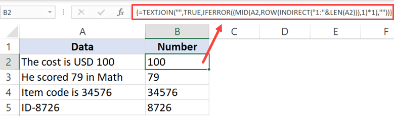
=TEXTJOIN("",TRUE,IFERROR((MID(A2,ROW(INDIRECT("1:"&LEN(A2))),1)*1),""))
This is an array formula, so you need to use ‘Control + Shift + Enter‘ instead of using Enter.
In case there are no numbers in the text string, this formula would return a blank (empty string).
How does this formula work?
Let me break this formula and try and explain how it works:
- ROW(INDIRECT(“1:”&LEN(A2))) – this part of the formula would give a series of numbers starting from one. The LEN function in the formula returns the total number of characters in the string. In the case of “The cost is USD 100”, it will return 19. The formulas would thus become ROW(INDIRECT(“1:19”). The ROW function will then return a series of numbers – {1;2;3;4;5;6;7;8;9;10;11;12;13;14;15;16;17;18;19}
- (MID(A2,ROW(INDIRECT(“1:”&LEN(A2))),1)*1) – This part of the formula would return an array of #VALUE! errors or numbers based on the string. All the text characters in the string become #VALUE! errors and all numerical values stay as-is. This happens as we have multiplied the MID function with 1.
- IFERROR((MID(A2,ROW(INDIRECT(“1:”&LEN(A2))),1)*1),””) – When IFERROR function is used, it would remove all the #VALUE! errors and only the numbers would remain. The output of this part would look like this – {“”;””;””;””;””;””;””;””;””;””;””;””;””;””;””;””;1;0;0}
- =TEXTJOIN(“”,TRUE,IFERROR((MID(A2,ROW(INDIRECT(“1:”&LEN(A2))),1)*1),””)) – The TEXTJOIN function now simply combines the string characters that remains (which are the numbers only) and ignores the empty string.
Pro Tip: If you want to check the output of a part of the formula, select the cell, press F2 to get into the edit mode, select the part of the formula for which you want the output and press F9. You will instantly see the result. And then remember to either press Control + Z or hit the Escape key. DO NOT hit the enter key.
Download the Example File
You can also use the same logic to extract the text part from an alphanumeric string. Below is the formula that would get the text part from the string:
=TEXTJOIN("",TRUE,IF(ISERROR(MID(A2,ROW(INDIRECT("1:"&LEN(A2))),1)*1),MID(A2,ROW(INDIRECT("1:"&LEN(A2))),1),""))
A minor change in this formula is that IF function is used to check if the array we get from MID function are errors or not. If it’s an error, it keeps the value else it replaces it with a blank.
Then TEXTJOIN is used to combine all the text characters.
Caution: While this formula works great, it uses a volatile function (the INDIRECT function). This means that in case you use this with a huge dataset, it may take some time to give you the results. It’s best to create a backup before you use this formula in Excel.
Extract Numbers from String in Excel (for Excel 2013/2010/2007)
If you have Excel 2013. 2010. or 2007, you can not use the TEXTJOIN formula, so you will have to use a complicated formula to get this done.
Suppose you have a dataset as shown below and you want to extract all the numbers in the string in each cell.
The below formula will get this done:
=IF(SUM(LEN(A2)-LEN(SUBSTITUTE(A2, {"0","1","2","3","4","5","6","7","8","9"}, "")))>0, SUMPRODUCT(MID(0&A2, LARGE(INDEX(ISNUMBER(--MID(A2,ROW(INDIRECT("$1:$"&LEN(A2))),1))* ROW(INDIRECT("$1:$"&LEN(A2))),0), ROW(INDIRECT("$1:$"&LEN(A2))))+1,1) * 10^ROW(INDIRECT("$1:$"&LEN(A2)))/10),"")
In case there is no number in the text string, this formula would return blank (empty string).
Although this is an array formula, you don’t need to use ‘Control-Shift-Enter’ to use this. A simple enter works for this formula.
Credit to this formula goes to the amazing Mr. Excel forum.
Again, this formula will extract all the numbers in the string no matter the position. For example, if the text is “The price of 10 tickets is USD 200”, it will give you 10200 as the result.
Caution: While this formula works great, it uses a volatile function (the INDIRECT function). This means that in case you use this with a huge dataset, it may take some time to give you the results. It’s best to create a backup before you use this formula in Excel.
Separate Text and Numbers in Excel Using VBA
If separating text and numbers (or extracting numbers from the text) is something you have to often, you can also use the VBA method.
All you need to do is use a simple VBA code to create a custom User Defined Function (UDF) in Excel, and then instead of using long and complicated formulas, use that VBA formula.
Let me show you how to create two formulas in VBA – one to extract numbers and one to extract text from a string.
Extract Numbers from String in Excel (using VBA)
In this part, I will show you how to create the custom function to get only the numeric part from a string.
Below is the VBA code we will use to create this custom function:
Function GetNumeric(CellRef As String)
Dim StringLength As Integer
StringLength = Len(CellRef)
For i = 1 To StringLength
If IsNumeric(Mid(CellRef, i, 1)) Then Result = Result & Mid(CellRef, i, 1)
Next i
GetNumeric = Result
End Function
Here are the steps to create this function and then use it in the worksheet:
Now, you will be able to use the GetText function in the worksheet. Since we have done all the heavy lifting in the code itself, all you need to do is use the formula =GetNumeric(A2).
This will instantly give you only the numeric part of the string.
Note that since the workbook now has VBA code in it, you need to save it with .xls or .xlsm extension.
Download the Example File
In case you have to use this formula often, you can also save this to your Personal Macro Workbook. This will allow you to use this custom formula in any of the Excel workbooks that you work with.
Extract Text from a String in Excel (using VBA)
In this part, I will show you how to create the custom function to get only the text part from a string.
Below is the VBA code we will use to create this custom function:
Function GetText(CellRef As String)
Dim StringLength As Integer
StringLength = Len(CellRef)
For i = 1 To StringLength
If Not (IsNumeric(Mid(CellRef, i, 1))) Then Result = Result & Mid(CellRef, i, 1)
Next i
GetText = Result
End Function
Here are the steps to create this function and then use it in the worksheet:
Now, you will be able to use the GetNumeric function in the worksheet. Since we have done all the heavy lifting in the code itself, all you need to do is use the formula =GetText(A2).
This will instantly give you only the numeric part of the string.
Note that since the workbook now has VBA code in it, you need to save it with .xls or .xlsm extension.
In case you have to use this formula often, you can also save this to your Personal Macro Workbook. This will allow you to use this custom formula in any of the Excel workbooks that you work with.
In case you’re using Excel 2013 or prior versions and don’t have
You May Also Like the Following Excel Tutorials:
- CONCATENATE Excel Ranges (with and without separator).
- A Beginner’s Guide to Using For Next Loop in Excel VBA.
- Using Text to Columns in Excel.
- How to Extract a Substring in Excel (Using TEXT Formulas).
- Excel Macro Examples for VBA Beginners.
- Separate Text and Numbers in Excel
Extracting numbers from a list of cells with mixed text is a common data cleaning task.
Unfortunately, there is no direct menu or function created in Excel to help us accomplish this.
In this tutorial we will look at three cases where you might have a list of mixed text, from which you might want to extract numbers:
- When the number is always at the end of the text
- When the number is always at the beginning of the text
- When the number can be anywhere in the text
We will look at three different formulas that can be used to extract the numbers in each case.
At the end of the tutorial, we will also take a look at some VBA code that you can use to accomplish the same.
Brace yourself, this might get a little complex!
Extracting a Number from Mixed Text when Number is Always at the End of the Text
Consider the following example:

Here, each cell has a mix of text and numbers, with the number always appearing at the end of the text. In such cases, we will need to use a combination of nested Excel functions to extract the numbers.
The functions we will use are:
- FIND – This function searches for a character or string in another string and returns its position.
- MIN – This function returns the smallest value in a list.
- LEFT – This function extracts a given number of characters from the left side of a string.
- SUBSTITUTE – This function replaces a particular substring of a given text with another substring.
- IFERROR – This function returns an alternative result or formula if it finds an error in a given formula.
Essentially, we will be using the above functions altogether to perform the following sequence of tasks:
- Find the position of the first numeric value in the given cell
- Extract and remove the text part of the given cell (by removing everything to the left of the first numeric digit)
The formula that we will use to extract the numbers from cell A2 is as follows:
=SUBSTITUTE(A2,LEFT(A2,MIN(IFERROR(FIND({0,1,2,3,4,5,6,7,8,9},A2),""))-1),"")
Let us break down this formula to understand it better. We will go from the inner functions to the outer functions:
- FIND({0,1,2,3,4,5,6,7,8,9},A2)
This function tries to find the positions of all the numbers (0-9) in the cell A2. Thus it returns an arrayformula:
{#VALUE!,#VALUE!,#VALUE!,#VALUE!,#VALUE!,#VALUE!,9,7,8,#VALUE!}
It returns a #VALUE! error for all digits except the 7th, 8th, and 9th digits because it was not able to find these numbers (0,1,2,3,4,5,9) in cell A2. It simply returns the positions of numbers 6,7 and 8 which are the 9th, 7th, and 8th characters respectively in A2.
- IFERROR(FIND({0,1,2,3,4,5,6,7,8,9},A2),””)
Next, the IFERROR function replaces all the error elements of the array with a blank (“”). As such it returns the arrayformula:
{“”,””,””,””,””,””,9,7,8,””}
- MIN(IFERROR(FIND({0,1,2,3,4,5,6,7,8,9},A2),””))
After this the MIN function finds the array element with least value. This is basically the position of the first numeric character in A2. The function now returns the value 7.
- LEFT(A2,MIN(IFERROR(FIND({0,1,2,3,4,5,6,7,8,9},A2),””))-1)
At this point we want to extract all text characters from A2 (so that we can remove them). So we want the LEFT function to extract all the characters starting backwards from the 7-1= 6th character. Thus we use the above formula. The result we get at this point is “arnold”. Notice we subtracted 1 from the second parameter of the LEFT function.
- SUBSTITUTE(A2,LEFT(A2,MIN(IFERROR(FIND({0,1,2,3,4,5,6,7,8,9},A2),””))-1),””)
Now all that’s left to do is remove the string obtained, by replacing it with a blank. This can be easily achieved by using the SUBSTITUTE function: We finally get the numeric characters in the mixed text, which is “786”.
Once you are done entering the formula, make sure you press CTRL+SHIFT+Enter, instead of just the return key. This is because the formula involves arrays.
In a nutshell, here’s what’s happening when you break down the formula:
=SUBSTITUTE(A2,LEFT(A2,MIN(IFERROR(FIND({0,1,2,3,4,5,6,7,8,9},A2),””))-1),””)
=SUBSTITUTE(A2,LEFT(A2,MIN(IFERROR({{#VALUE!,#VALUE!,#VALUE!,#VALUE!,#VALUE!,#VALUE!,9,7,8,#VALUE!}),””))-1),””)
=SUBSTITUTE(A2,LEFT(A2,MIN({“”,””,””,””,””,””,9,7,8,””}))-1),””)
=SUBSTITUTE(A2,”arnold”,””)
=786
When you drag the formula down to the rest of the cells, here’s the result you get:

Also read: How to Generate Random Letters in Excel?
Extracting a Number from Mixed Text when Number is Always at the Beginning of the Text
Now let us consider the case where the numbers are always at the beginning of the Text.
Consider the following example:

Here, each cell has a mix of text and numbers, with the number always appearing at the beginning of the text. In such cases, we will again need to use a combination of nested Excel functions to extract the numbers.
In addition to the functions we used in the previous formula, we are going to use two additional functions. These are:
- MAX – This function returns the largest value in a list
- RIGHT – This function extracts a given number of characters from the right side of a string
- LEN – This function finds the length of (number of characters in) a given string.
Essentially, we will be using these functions altogether to perform the following sequence of tasks:
- Find the position of the last numeric value in the given cell
- Extract and remove the text part of the given cell (by removing everything to the right of the last numeric digit)
The formula that we will use to extract the numbers from cell A2 is as follows:
=SUBSTITUTE(A2,RIGHT(A2,LEN(A2)-MAX(IFERROR(FIND({0,1,2,3,4,5,6,7,8,9},A2),""))),"")
Let us break down this formula to understand it better. We will go from the inner functions to the outer functions:
- FIND({0,1,2,3,4,5,6,7,8,9},A2)
This function tries to find the positions of all the numbers (0-9) in the cell A2. Thus it returns an arrayformula:
{#VALUE!,#VALUE!,1,#VALUE!,#VALUE!,2,#VALUE!,#VALUE!,#VALUE!,#VALUE!}
It returns a #VALUE! error for all digits except the 3rd and 6th digits because it was not able to find these numbers (0,1,3,4,6,7,8,9) in cell A2. It simply returns the positions of numbers 2 and 5 which are the 1st and 2nd characters respectively in A2.
- IFERROR(FIND({0,1,2,3,4,5,6,7,8,9},A2),””)
Next, the IFERROR function replaces all the error elements of the array with a blank. As such it returns the array formula:
{“”,””,1,””,””,2,””,””,””,””}
- MAX(IFERROR(FIND({0,1,2,3,4,5,6,7,8,9},A2),””))
After this the MAX function finds the array element with the highest value. This is basically the position of the last numeric character in A2. The function now returns the value 2.
- LEN(A2)-MAX(IFERROR(FIND({0,1,2,3,4,5,6,7,8,9},A2),””))
At this point we want to extract all text characters from A2 (so that we can remove them). We need to specify how many characters we want to remove. This is obtained by computing the length of the string in A2 minus the position of the last numeric value.Thus we will get the value 8-2 = “6”.
- RIGHT(A2,LEN(A2)-MAX(IFERROR(FIND({0,1,2,3,4,5,6,7,8,9},A2),””)))
We can now use the RIGHT function to extract 6 characters starting from the 2nd character onwards. The result we get at this point is “arnold”.
- SUBSTITUTE(A2,RIGHT(A2,LEN(A2)-MAX(IFERROR(FIND({0,1,2,3,4,5,6,7,8,9},A2),””))),””)
Now all that’s left to do is remove this string by replacing it with a blank. This is easily achieved by using the SUBSTITUTE function. We finally get the numeric characters in the mixed text, which is “25”.
Again, once you are done entering the formula, don’t forget to press CTRL+SHIFT+Enter, instead of just the return key.
In a nutshell, here’s what’s happening when you break down the formula:
=SUBSTITUTE(A7,RIGHT(A7,LEN(A7)-MAX(IFERROR(FIND({0,1,2,3,4,5,6,7,8,9},A7),””))),””)
=SUBSTITUTE(A7,RIGHT(A7,LEN(A7)-MAX(IFERROR({#VALUE!,#VALUE!,1,#VALUE!,#VALUE!,2,#VALUE!,#VALUE!,#VALUE!,#VALUE!}
),””))),””)
=SUBSTITUTE(A7,RIGHT(A7,LEN(A7)-MAX({“”,””,1,””,””,2,””,””,””,””}
)),””)
=SUBSTITUTE(A7,RIGHT(A7,LEN(A7)-2),””)
=SUBSTITUTE(A7,RIGHT(A7,8-2),””)
=SUBSTITUTE(A7,”arnold”,””)
=25
When you drag the formula down to the rest of the cells, here’s the result you get:

Extracting a Number from Mixed Text when Number can be Anywhere in the Text
Finally let us consider the case where the numbers can be anywhere in the text, be it the beginning, end or middle part of the text.
Let’s take a look at the following example:

Here, each cell has a mix of text and numbers, where the number appears in any part of the text. In such cases, we will need to use a combination of nested Excel functions to extract the numbers.
Here are the functions that we are going to use this time:
- INDIRECT – This function simply returns a reference to a range of values.
- ROW – This function returns a row number of a reference.
- MID – This function extracts a given number of characters from the middle of a string.
- TEXTJOIN – This function combines text from multiple ranges or strings using a specified delimiter between them.
Note that the formula discussed in this section will work only in Excel version 2016 onwards as it uses the newly introduced TEXTJOIN function. If you are using an older version of Excel, then you may consider using the VBA method instead (discussed in the next section).
In this method, we will essentially be using the above functions altogether to perform the following sequence of tasks:
- Break up the given text into an array of individual characters
- Find out and remove all characters that are not numbers
- Combine the remaining characters into a full number
The formula that we will use to extract the numbers from cell A2 is as follows:
=TEXTJOIN("",TRUE,IFERROR(MID(A2,ROW(INDIRECT("1:"&LEN(A2))),1)*1,""))
Let us break down this formula to understand it better. We will go from the inner functions to the outer functions:
- LEN(A2)
This function finds the length of the string in cell A2. In our case it returns 13.
- INDIRECT(“1:”&LEN(A2))
This function just returns a reference to all the rows from row 1 to row 12.
- ROW(INDIRECT(“1:”&LEN(A2)))
Now this function returns the row numbers of each of these rows. In other words, it simply returns an array of numbers 1 to 12. This function thus returns the array:
{1;2;3;4;5;6;7;8;9;10;11;12;13}
Note: We use the ROW() function instead of simply hard-coding an array of numbers 1 to 12 because we want to be able to customize this formula depending on the size of the string being worked on. This will ensure that the function adjusts itself when copied to another cell. ·
- MID(A2,ROW(INDIRECT(“1:”&LEN(A2))),1)
Next the MID function extracts the character from A2 that corresponds to each position specified in the array. In other words, it returns an array containing each character of the text in A2 as a separate element, as follows:
{“a”;”r”;”n”;”o”;”l”;”d”;”1″;”4″;”3″;”b”;”l”;”u”;”e”}
- IFERROR(MID(A2,ROW(INDIRECT(“1:”&LEN(A2))),1)*1,””)
After this, the IFERROR function replaces all the elements of the array that are non-numeric. This is because it checks if the array element can be multiplied by 1. If the element is a number, it can easily be multiplied to return the same number. But if the element is a non-numeric character, then it cannot be multiplied with 1 and thus returns an error.
The IFERROR function here specifies that if an element gives an error on multiplication, the result returned will be blank. As such it returns the arrayformula:
{“”;””;””;””;””;””;1;4;3;””;””;””;””}
- TEXTJOIN(“”,TRUE,IFERROR(MID(A2,ROW(INDIRECT(“1:”&LEN(A2))),1)*1,””))
Finally, we can simply combine the array elements together using the TEXTJOIN function. The TEXTJOIN function here combines the string characters that remain (which are the numbers only) and ignores the empty string characters. We finally get the numeric characters in the mixed text, which is “143”.
Once you are done entering the formula, don’t forget to press CTRL+SHIFT+Enter, instead of just the return key.
In a nutshell, here’s what’s happening when you break down the formula:
=TEXTJOIN(“”,TRUE,IFERROR(MID(A2,ROW(INDIRECT(“1:”&LEN(A2))),1)*1,””))
=TEXTJOIN(“”,TRUE,IFERROR(MID(A2,ROW(INDIRECT(“1:”&13)),1)*1,””))
=TEXTJOIN(“”,TRUE,IFERROR(MID(A2,{1;2;3;4;5;6;7;8;9;10;11;12;13},1)*1,””))
=TEXTJOIN(“”,TRUE,IFERROR({“a”;”r”;”n”;”o”;”l”;”d”;”1″;”4″;”3″;”b”;”l”;”u”;”e”}
*1,””))
=TEXTJOIN(“”,TRUE,IFERROR(MID(A2,{1;2;3;4;5;6;7;8;9;10;11;12;13},1)*1,””))
=TEXTJOIN(“”,TRUE, {“”;””;””;””;””;””;1;4;3;””;””;””;””})
=143
When you drag the formula down to the rest of the cells, here’s the result you get:

Using VBA to Extract Number from Mixed Text in Excel
The above method works well enough in extracting numbers from anywhere in a mixed text.
However, it requires one to use the TEXTJOIN function, which is not available in older Excel versions (versions before Excel 2016).
If you’re on a version of Excel that does not support TEXTJOIN, then you can, instead, use a snippet of VBA code to get the job done.
If you have never used VBA before, don’t worry. All you need to do is copy the code below into your VBA developer window and run it on your worksheet data.
Here’s the code that you will need to copy:
'Code by Steve Scott from spreadsheetplanet.com
Function ExtractNumbers(CellRef As String)
Dim StringLength As Integer
StringLength = Len(CellRef)
For i = 1 To StringLength
   If (IsNumeric(Mid(CellRef, i, 1))) Then Result = Result & Mid(CellRef, i, 1)
Next i
ExtractNumbers = Result
End Function
The above code creates a user-defined function called ExtractNumbers() that you can use in your worksheet to extract numbers from mixed text in any cell.
To get to your VBA developer window, follow these steps:
- From the Developer tab, select Visual Basic.

- Once your VBA window opens, Click Insert->Module. That’s it, you can now start coding.

Type or copy-paste the above lines of code into the module window. Your code is now ready to run.

Now, whenever you want to extract numbers from a cell, simply type the name of the function, passing the cell reference as a parameter. So to extract numbers from a cell A2, you will simply need to type the function as follows in a cell:
=ExtractNumbers(A2)

Explanation of the Code
Now let us take some time to understand how this code works.
- In this code, we defined a function named ExtractNumbers, that takes the string in the cell we want to work on. We assigned the name CellRef to this string.
Function ExtractNumbers(CellRef As String)
- We created a variable named StringLength, that will hold the length of the string, CellRef.
Dim StringLength As Integer
StringLength = Len(CellRef)
- Next, we loop through each character in the string CellRef and find out if it is a number. We use the function Mid(CellRef, i, 1) to extract a character from the string at each iteration of the loop. We also use the IsNumeric() function to find out if the extracted character is a number. Each extracted numeric character is combined together into a string called Result.
For i = 1 To StringLength
If (IsNumeric(Mid(CellRef, i, 1))) Then Result = Result & Mid(CellRef, i, 1)
Next i
- This Result is then returned by the function.
ExtractNumbers = Result
Note that since the workbook now has VBA code in it, you need to save it with .xls or .xlsm extension.
You can also choose to save this to your Personal Macro Workbook, if you think you will be needing to run this code a lot. This will allow you to run the code on any Excel workbook of yours.
Well, that was a lot!
In this tutorial, we showed you how to extract numbers from mixed text in excel.
We saw three cases where the numbers are situated in different parts of the text. We also showed you how to use VBA to get the task done quickly.
Other Excel articles you may also like:
- How to Extract URL from Hyperlinks in Excel (Using VBA Formula)
- How to Reverse a Text String in Excel (Using Formula & VBA)
- How to Add Text to the Beginning or End of all Cells in Excel
- How to Remove Text after a Specific Character in Excel (3 Easy Methods)
- How to Separate Address in Excel?
- How to Extract Text After Space Character in Excel?
- How to Find the Last Space in Text String in Excel?
- How to Remove Space before Text in Excel