
Excel for Microsoft 365 Excel for Microsoft 365 for Mac Excel for the web Excel 2021 Excel 2021 for Mac Excel 2019 Excel 2019 for Mac Excel 2016 Excel 2016 for Mac Excel 2013 Excel 2010 Excel 2007 Excel for Mac 2011 Excel Starter 2010 More…Less
This article describes the formula syntax and usage of the DATEVALUE function in Microsoft Excel.
Description
The DATEVALUE function converts a date that is stored as text to a serial number that Excel recognizes as a date. For example, the formula =DATEVALUE(«1/1/2008») returns 39448, the serial number of the date 1/1/2008. Remember, though, that your computer’s system date setting may cause the results of a DATEVALUE function to vary from this example
The DATEVALUE function is helpful in cases where a worksheet contains dates in a text format that you want to filter, sort, or format as dates, or use in date calculations.
To view a date serial number as a date, you must apply a date format to the cell. Find links to more information about displaying numbers as dates in the See Also section.
Syntax
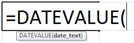
DATEVALUE(date_text)
The DATEVALUE function syntax has the following arguments:
-
Date_text Required. Text that represents a date in an Excel date format, or a reference to a cell that contains text that represents a date in an Excel date format. For example, «1/30/2008» or «30-Jan-2008» are text strings within quotation marks that represent dates.
Using the default date system in Microsoft Excel for Windows, the date_text argument must represent a date between January 1, 1900 and December 31, 9999. The DATEVALUE function returns the #VALUE! error value if the value of the date_text argument falls outside of this range.
If the year portion of the date_text argument is omitted, the DATEVALUE function uses the current year from your computer’s built-in clock. Time information in the date_text argument is ignored.
Remarks
-
Excel stores dates as sequential serial numbers so that they can be used in calculations. By default, January 1, 1900 is serial number 1, and January 1, 2008 is serial number 39448 because it is 39,447 days after January 1, 1900.
-
Most functions automatically convert date values to serial numbers.
Example
Copy the example data in the following table, and paste it in cell A1 of a new Excel worksheet. For formulas to show results, select them, press F2, and then press Enter. If you need to, you can adjust the column widths to see all the data.
|
Data |
||
|---|---|---|
|
11 |
||
|
3 |
||
|
2011 |
||
|
Formula |
Description |
Result |
|
=DATEVALUE(«8/22/2011») |
Serial number of a date entered as text. |
40777 |
|
=DATEVALUE(«22-MAY-2011») |
Serial number of a date entered as text. |
40685 |
|
=DATEVALUE(«2011/02/23») |
Serial number of a date entered as text. |
40597 |
|
=DATEVALUE(«5-JUL») |
Serial number of a date entered as text, using the 1900 date system, and assuming the computer’s built-in clock returns 2011 as the current year. |
39634 |
|
=DATEVALUE(A2 & «/» & A3 & «/» & A4) |
Serial number of a date created by combining the values in cells A2, A3, and A4. |
40850 |
Need more help?
Want more options?
Explore subscription benefits, browse training courses, learn how to secure your device, and more.
Communities help you ask and answer questions, give feedback, and hear from experts with rich knowledge.
Функция DATEVALUE (ДАТАЗНАЧ) в Excel используется для тех ситуаций, когда дата в ячейке указана в виде текста. С её помощью Excel конвертирует текстовое значение даты в число, которое система распознает как дату.
Содержание
- Какие данные отображает
- Синтаксис
- Аргументы
- Дополнительная информация
- Примеры использования функции DATEVALUE (ДАТАЗНАЧ)
- Пример №1. Преобразование даты в текстовом формате в число
- Пример №2. Преобразование даты в текстовом формате с помощью формулы
- Пример №3. Использование функции без указания года
- Пример №4. Использование функции без указания дня
Какие данные отображает
Функция возвращает дату в виде числового значения, понятного по формату для Excel. Например, если мы используем функцию =DATEVALUE («1/1/2016») или =ДАТАЗНАЧ(«1/1/2016») , она будет возвращать число 42370, которое является числовым значением даты 01-01-2016.
Синтаксис
=DATEVALUE (“date_text”) — английская версия
=ДАТАЗНАЧ («дата_как_текст») — русская версия
Аргументы
date_text (дата_как_текст): это аргумент даты указанной в ячейке в формате текста или результат какой-либо формулы в виде текста;
- для правильной работы функции, текст, который нам необходимо преобразовать в формулу важно указать в кавычках (прим. “01/01/2016”);
- если date_text это результат какого-либо вычисления, важно чтобы ячейка была в текстовом формате, для корректной работы функции.
Дополнительная информация
DATEVALUE (ДАТАЗНАЧ) возвращает числовое значение даты:
- Например: формула =DATEVALUE(“1/1/2014”) или =ДАТАЗНАЧ(“1/1/2014”) преобразует значение в число 41640, которое означает дату 1 января 2014 в формате даты.
- Если вы указываете дату без дня (прим. =DATEVALUE(“1/2014”) или =ДАТАЗНАЧ(“1/1/2014”), а только месяц и год, система вернет числовое значение даты как первого дня указанного месяца — 41640, что для Excel будет означать как 01.01.2014.
- Если вы не используете значение года (прим. =DATEVALUE(“01/04”) или =ДАТАЗНАЧ(“01/04”), Excel автоматически присвоит текущий год (указанный в настройках даты и времени вашей ОС).
- Формат значения даты, которую выдает функция, зависит от настроек вашей ОС. Например в России (по умолчанию) при преобразовании даты 01/03/2016 это будет 1 Марта 2016, в США это 3 Января 2016.
Примеры использования функции DATEVALUE (ДАТАЗНАЧ)
Пример №1. Преобразование даты в текстовом формате в число

В приведенном выше примере, формула возвращает числовое значение даты введенной в кавычках. Введенная дата должна быть в текстовом формате, иначе Excel возвращает “#VALUE!” ошибку.
Обратите внимание, что значение, возвращаемое функцией зависит от настройки часов вашей системы. Если дата указана в формате ДД-ММ-ГГГГ значит «01-06-2016» будет отображать как 1 июня 2016 года, но для формата даты ММ-ДД-ГГГГ дата будет отображаться как 6 января 2016.
Больше лайфхаков в нашем Telegram Подписаться
Пример №2. Преобразование даты в текстовом формате с помощью формулы
Когда дата введена как текст в ячейку, вы можете использовать функцию DATAVALUE (ДАТАЗНАЧ), чтобы получить числовое значение даты. Обратите внимание, что дата должна быть в текстовом формате.
В приведенном выше примере, формула преобразует “1-6-16” и “1-июня-16” — это значение указанное в формате даты.
Эта функция полезна, когда у вас есть дата в текстовом формате, по которой вы хотите фильтровать, сортировать данные в таблице. В текстовом формате, вы не сможете сортировать даты и проводить вычисления в Excel, так как система будет рассматривать его как текст, а не число.
Пример №3. Использование функции без указания года
Если значение года не указано, то система использует текущий год при отображении значения даты (текущий год 2016 в указанном примере).
Пример №4. Использование функции без указания дня
Если в дате не указан день, то формула использует первый день месяца.
В приведенных выше примерах, когда мы вводим число «6-16», система возвращает число 42522, которое является значением даты на 1 июня 2016 года.
The DATEVALUE function in Excel shows any given date in absolute format. This function takes an argument in the form of date text normally not represented by Excel as a date and converts it into a format that Excel can recognize as a date. This function helps make the given dates in a similar date format for calculations. The method to use this function is =DATEVALUE( date_text).
For example, if we insert “31Dec2021” as the text date, the DATEVALUE function in Excel would give us the result as “31/12/2021”
Table of contents
- DATEVALUE Function in Excel
- Syntax
- How to use the DATEVALUE Function in Excel? (With Examples)
- Example #1
- Example #2
- Things to Remember
- Recommended Articles
Syntax
Arguments
- date_text: A valid date in text format. The date_text argument can be entered directly or provided as a cell reference. If date_text is a cell reference, the cell value must be formatted as text. If date_text is entered directly, it should be enclosed in quotes. The date_text argument should only refer to the date between January 1, 1900, and December 31, 9999.
- Return: It returns a serial number representing a particular date in Excel. It will produce a #VALUE! Error if date_text refers to a cell that does not contain a date formatted as text. If the input data is outside the range of Excel, the DATEVALUE in Excel will return #VALUE! Error.
How to use the DATEVALUE Function in Excel? (With Examples)
The Excel DATEVALUE function is very simple and easy to use. Let us understand the working of DATEVALUE in Excel by some examples.
You can download this DATEVALUE Function Excel Template here – DATEVALUE Function Excel Template
Example #1
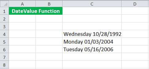
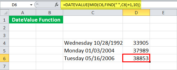
IIn this Excel DATEVALUE function example, suppose we have the day and date given in cell C4:C6. Now, we want to extract the date and get the serial number of the dates.
We can use the following Excel DATEVALUE function to extract the date for the first one and return the date value of the corresponding date:
= DATEVALUE ( MID (C4, FIND (” ” , C4) + 1, 10 ) )
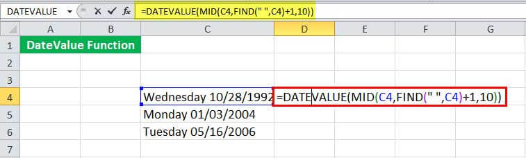
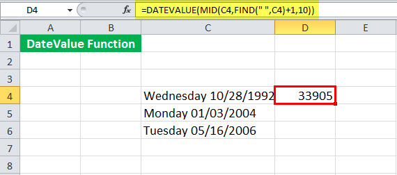
It will return the serial number for the date 28/10/1992.
We need to drag it to the rest of the cells to get the date value for the remaining ones.
Now, let us see the DATEVALUE function in detail:
= DATEVALUE ( MID (C4, FIND (” “, C4) + 1, 10 ) )
- FIND (” “, C4) will find the location of the 1st space occurring in cell C4.

It will return to 10.

- FIND (” “, C4) + 1 will give the starting location of the date.
- MID (C4, FIND (” “, C4) + 1, 10 ) will chop and return the cell text from the 10th position to 10 places forward. For example, it will return on 28/10/1992.
- DATEVALUE ( MID (C4, FIND (” ”, C4) + 1, 10 ) ) will finally convert the input date text to the serial number and return 33905.
Example #2
In this Excel DATEVALUE function example, suppose we have the data of sales collected at some time interval. The start date is 1 March 2018. Then, we collected the sales data on 5 March 2018. So, this represents the sales that have taken place between 1 and 5 March 2018. Next, we collected data on 11 March 2018, representing the sales between 5-11 March 2018.
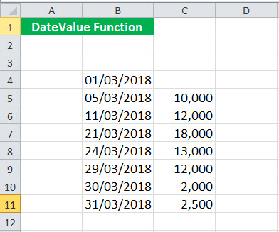
Now, we are not interested in the dates. Instead, we want to know how many days the sales were 10,000 (cell B5). To get the number of days, you could use the following DATEVALUE function:
= DATEVALUE (B5) – DATEVALUE (B4)
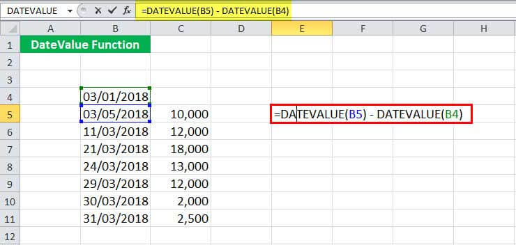
This DATEVALUE function in Excel will return 4.
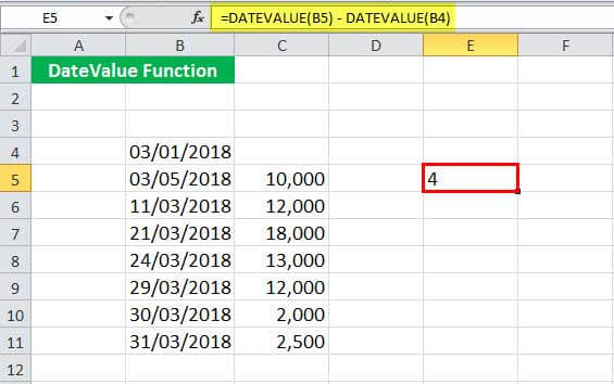
We can now drag it to the rest of the cells.
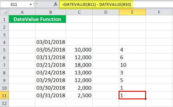
It is worth mentioning that with each day, the serial number of the date increases by 1. Since Excel recognizes the dates only after 1 Jan 1900, the serial number of this date is 1. For 2 Jan 1990, it is 2, and so on. Therefore, subtracting any two serial numbers will return the number of days between them.
Things to Remember
- It converts any given date into a serial number, representing an Excel date.
- If given a cell reference, the cell must be formatted as text.
- This function will return a #VALUE! Error if date_text refers to a cell that does not contain a date or is not formatted as text.
- It accepts a date only between January 1, 1900, and December 31, 9999.
Recommended Articles
This article is a guide to DATEVALUE Function in Excel. We discuss the DATEVALUE formula in Excel, using the DATEVALUE function and Excel examples, and downloadable excel templates. You may also look at these useful functions in Excel: –
- Insert Date in Excel
- EDATE Function
- DATE Excel Function | Examples
- TODAY’s Date Excel Function
- Apple Numbers vs. Excel
Reader Interactions
Excel DATE Function Overview

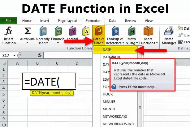
When to use Excel DATE Function
Excel DATE function can be used when you want to get the date value using the year, month and, day values as the input arguments. The input arguments can be entered manually, as cell reference that contains the dates, or as a result some formula.
What it Returns
It returns a serial number that represents a specific date in Excel. For example, if it returns 42370, it represents the date: 01 January 2016.
Syntax
=DATE(year, month, day)
Input Arguments
- year – the year to be used for the date.
- month – the month to be used for the date.
- day – the day to be used for the date.
Additional Notes (boring stuff.. but important to know)
- The result displayed in the cell would depend on the formatting of that cell. For example:
- If the cell is formatted as General, the result is displayed in the date format (remember dates are always stored as serial numbers but can be displayed in various formats).
- To get the result as a serial number, change the cell’s formatting to Number.
- It is recommended to use the four-digit year to avoid unwanted results. If the Year value used is less than 1900, Excel automatically adds 1900 to it. For example, if you use ten as the Year value, Excel makes it 1910.
- The Month value can be less than 0 or greater than 12. If the Month value is greater than 12, then Excel automatically adds that excess month to the next year. Similarly, if the month value is less than 0, the DATE function would automatically go back that many numbers of months.
- For example, DATE(2015,15,1) would return 1 March 2016. Similarly, DATE(2016,-2,1) would return October 1, 2015.
- Day value could be positive or negative. If the day value is negative, Excel automatically deducts that many days from the first day of the specified month. If it is more than the number of days in that month, then those extra days are added to the next month value. (example below).
Excel DATE Function – Examples
Here are X example of using the Excel DATE function:
Example 1: Getting the Date Serial number using Year, Month, and Day values
You can get the serial number of a date when you specify the Year, Month, and Day values.
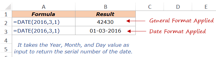
In the example above, the DATE function takes three arguments, 2016 as the year value, 3 as the month value, and 1 as the date value.
It returns 42430 when the cell is formatted as ‘General’, and returns 01-03-2016 when the cell is formatted as ‘Date’.
Note that Excel stores a date or time as a number.
The date format can vary based on your regional settings. For example, the date format in the US is DD-MM-YYYY, while in the UK it’s MM-DD-YYYY.
If you have the Year, Month, and Day values in cells in a worksheet, you can use the cell references as shown below:

Example 2: Using Negative Values for Month or Days
You can use negative values for month and days. When you use a negative value for a month, let’s say -1, it goes back by 1 month return its date.
For example, if you use the formula =DATE(2017,-1,1), it’ll return the date November 1, 2016, as goes back by one month. Similarly, you can use any negative number in months.

The same logic is followed when you use a month value that is more than 12. In that case, it goes to the next year and returns as the date after the months in excess of 12.
For example, if you use the formula =DATE(2016,14,1), it’ll return the date February 1, 2017.

Note: The date format shown in the examples above is based on my system’s settings (which is DD-MM-YYYY). It may vary based on your settings.
Similarly, you can also use negative day values or values that are more than 31, and accordingly, Excel DATE function would adjust the date.
Excel DATE Function – VIDEO
Other Useful Excel Functions:
- DATEVALUE Function: Excel DATEVALUE function is best suited for situations when a date is stored as text. This function converts the date from text format to a serial number that Excel recognizes as a date.
- NETWORKDAYS Function: Excel NETWORKDAYS function can be used when you want to get the number of working days between two given dates. It does not count the weekends between the specified dates (by default the weekend is Saturday and Sunday). It can also exclude any specified holidays.
- NETWORKDAYS.INTL Function: Excel NETWORKDAYS.INTL function can be used when you want to get the number of working days between two given dates. It does not count the weekends and holidays, both of which can be specified by the user. It also enables you to specify the weekend (for example, you can specify Friday and Saturday as the weekend, or only Sunday as the weekend).
- TODAY Function: Excel TODAY function can be used to get the current date. It returns a serial number that represents the current date.
- WEEKDAY Function: Excel WEEKDAY function can be used to get the day of the week as a number for the specified date. It returns a number between 1 and 7 that represents the corresponding day of the week.
- WORKDAY Function: Excel WORKDAY function can be used when you want to get the date after a given number of working days. By default, it takes Saturday and Sunday as the weekend
- WORKDAY.INTL Function: Excel WORKDAY.INTL function can be used when you want to get the date after a given number of working days. In this function, you can specify the weekend to be days other than Saturday and Sunday.
- DATEDIF Function: Excel DATEDIF function can be used when you want to calculate the number of years, months, or days between the two specified dates. A good example would be calculating the age.
You May Also Like the Following Excel Tutorials:
- Creating a holiday calendar in Excel.
- Excel Timesheet Calculator Template.
- Calendar Integrated with a To Do List Template.
- How to Automatically Insert Date and Time Stamp in Excel.
- How to Calculate Age in Excel using the date of birth.
- How to Convert Date to Text in Excel.
- MS Excel Functions Help – DATE.
- How to Add Months to Date in Excel
- How to Convert Text to Date in Excel (8 Easy Ways)
DATE in Excel (Table of Contents)
- DATE in Excel
- DATE Formula in Excel
- How to Use DATE Function in Excel?
Introduction to Excel DATE Function
The date function is quite helpful for creating the dates that consider Month, Year, and Day. We can feed any number here, and the Date function will create the date with respect to the value we feed in. This function is quite useful and helpful for structuring the date standards when we have multiple dates in multiple formats, and we want to standardize this with a single type for all.
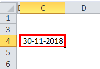
Let us look at the below simple examples. First, enter the number 43434 in excel and give the format as DD-MM-YYY.
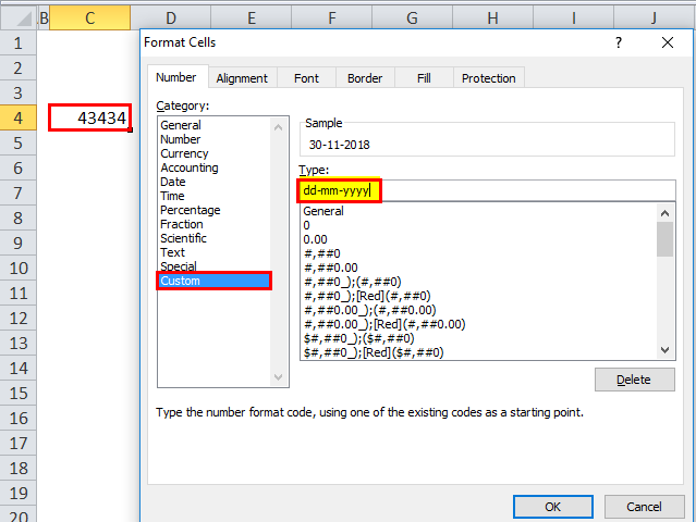
Once the above format is given, now look at how excel shows up that number.
Now give the format as [hh]:mm: ss, and the display will be as per the below image.
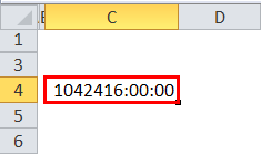
So excel completely works on numbers and their formats.
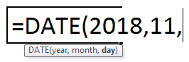
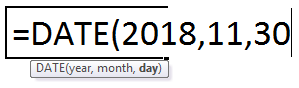
By using the DATE Function in Excel, we can create an accurate date. For example, =DATE (2018, 11, 14) would give the result as 14-11-2018.
DATE Formula in Excel
The Formula for the DATE Function in Excel is as follows:
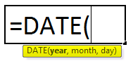
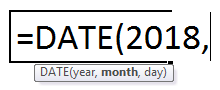
The Formula of DATE function includes 3 arguments, i.e. Year, Month, and Day.
1. Year: It is the mandatory parameter. A year is always a 4-digit number; since it is a number, we need not to specify the number in any double-quotes.
2. Month: This is also a mandatory parameter. A month should be a 2-digit number that can be supplied either directly to the cell reference or direct supply to the parameter.
3. Day: It is also a mandatory parameter. A day should be a 2-digit number.
How to Use DATE Function in Excel?
This DATE Function in Excel is very simple easy to use. Let us now see how to use the DATE Function in Excel with the help of some examples.
You can download this DATE Function Excel Template here – DATE Function Excel Template
Example #1
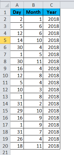
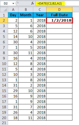
From the below data, create full date values. In the first column, we have days; in the second column, we have a month; and in the third column, we have a year. We need to combine these three columns and create a full date.
Enter the above into an excel sheet and apply the below formula to get the full date value.
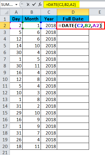
The Full DATE value is given below:
Example #2
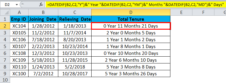
Find the difference between two days in terms of Total Years, Total Month, and Days. For example, assume you are working in an HR department in a company, and you have employee joining date and relieving date data. Next, you need to find the total tenure in the company. For example, 4 Years, 5 Months, 12 Days.
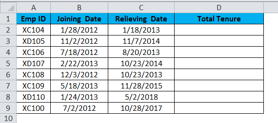
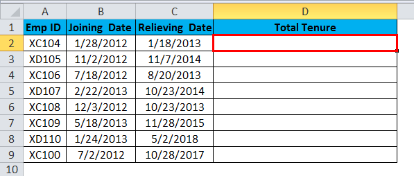
Here we need to use the DATEDIF function to get the result as per our wish. DATE function alone cannot do the job for us. If we just deduct the relieving date with the joining date, we get the only number of days they worked; we get in detail.
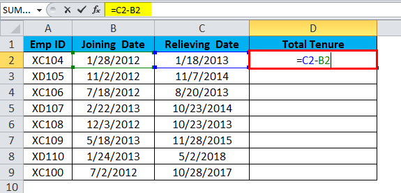
In order to get the full result, i.e. Total Tenure, we need to use the DATEDIF function.
DATEDIF function is an undocumented formula where there is no IntelliSense list for it. This can be useful to find the difference between year, month, and day.
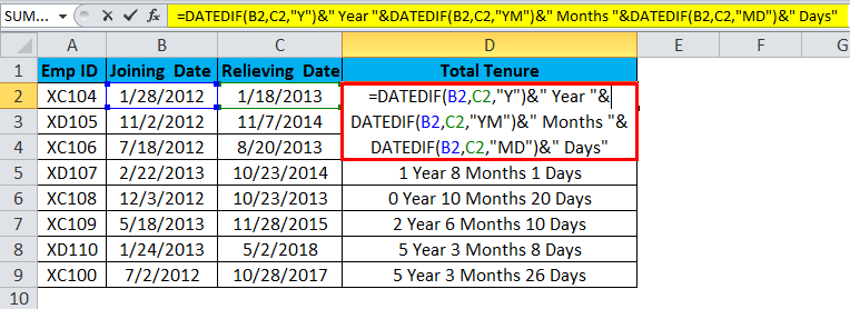
The formula looks like a lengthy one. However, I will break it down in detail.
Part 1: =DATEDIF (B2,C2, “Y”) this is the starting date and ending date, and “Y” means we need to know the difference between years.
Part 2: &” Year” This part is just added to a previous part of the foSo, forla. For example, if the first part gives, 4 then the result will be 4 Years.
Part 3: &DATEDIF(B2, C2, “YM”) Now, we found the difference between years. In this part of the formula, we are finding the difference between the months. “YM” can give the difference between months.
Part 4: &” Months” This is the addition to part 3. If the result of part 3 is 4, then this part will add Months to part 3, i.e. 3 Months
Part 5: “&DATEDIF(B2, C2,” MD”) now we have a difference between Year and the Month. In this part, we are finding the difference between the days. “MD” can give us that difference.
Part 6: &” Days” is added into part 5. If the result from part 5 is 25, then it will add Days to it. I.e. 25 Days.
Example #3
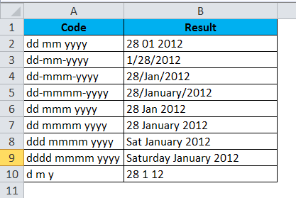
Now I will explain to you the different date formats in excel. There are many date formats in excel each show up the result differently.
VBA Example with Date in Excel:
Assume you are in the welfare team of the company, and you need to send birthday emails to your employees if there are any birthdays. However, sending each one of them is a tedious task. So here, I have developed a code to auto-send birthday wishes.
Below is the list of employees and their birthdays.
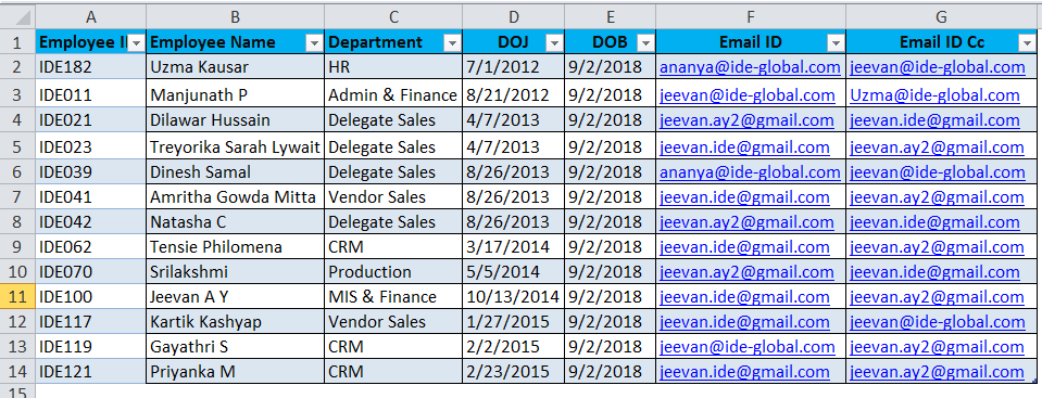
I have already written a code to send the birthday emails to everyone if there is any birthday today.
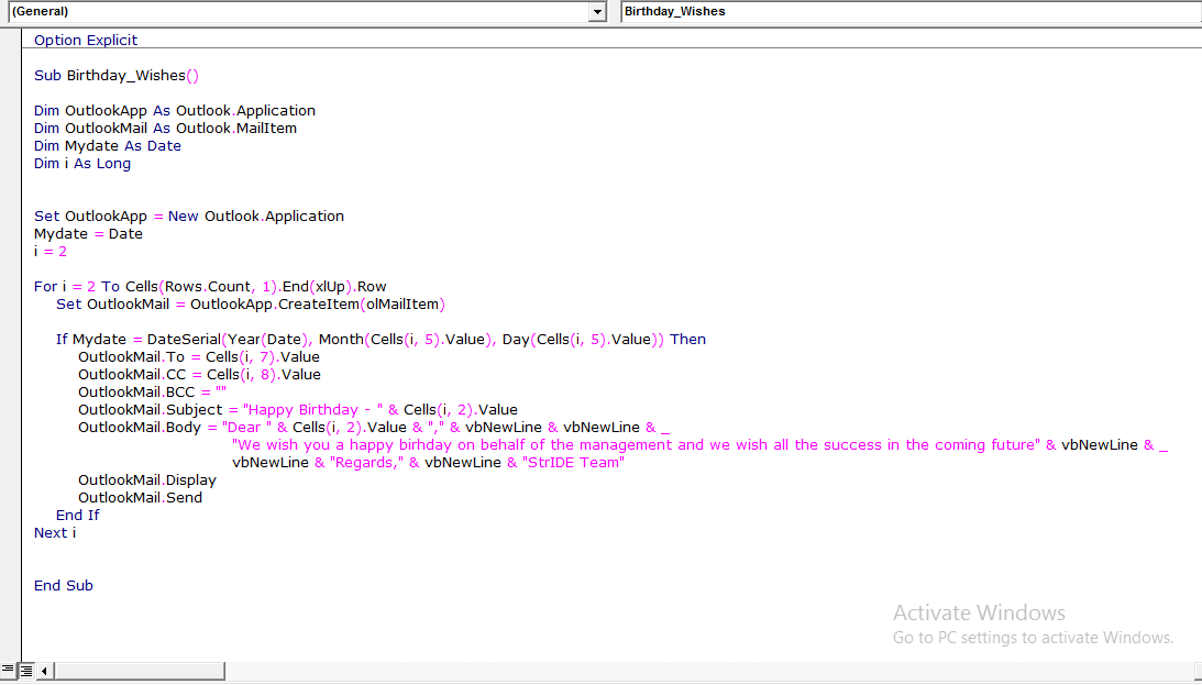
Write the above in your VBA module and save the workbook as a macro-enabled workbook.
Once the above code is written on the VBA module, save the workbook.
The only thing you need to do is add your data to the excel sheet and run the code every day you come to an office.
Things to Remember
- The given number should be >0 and <10000; otherwise, excel will give the error as #NUM!
- We can supply only numerical values. Anything other than numerical values, we will get eh error as #VALUE!
- Excel stores date as serial numbers and show the display according to the format.
- Always enter a full-year value. Do not enter any shortcut years like 18, 19, and 20, etc. Instead, enter the full year 2017, 2018, 2020
Recommended Articles
This is a guide to Excel DATE Function. Here we discuss the DATE Formula in Excel and how to use the DATE Function in Excel along with excel examples and downloadable excel templates. You may also look at these useful functions in excel –
- EDATE Excel Function
- Compare Dates in Excel
- Subtract Date In Excel
- VBA Date
For work with dates in Excel, in the category «Date and time» is defined in the functions section. Let`s consider the most prevalent functions in this category.
How Excel Processes Time
The Excel program «perceives» the date and time as an ordinary number. The spreadsheet converts to such number, equating the day to unity. As a result, the time value represents a fraction of unity. For example, 12. 00 — is 0. 5.
The date value to the spreadsheet converts to a number which equal to the number of days from January 1, 1900 (so the developers decided) to the specified date. For example, when converting the date 13. 04. 1987, the number is 31880. That is, from 1. 01. 1900 passed 31. 880 days.
This principle underlies in the basis of the calculations of the time data. To find the number of days between two dates, it`s enough to take an earlier period from a later time one.
The example of DATE function
You need to describe of the date value with compiling it with individual elements of numbers.
There is the syntax: year; month, day.
All arguments are required. They can be specified by numbers or by reference to cells with the corresponding numeric data: for the year — from 1900 to 9999; for the month — from 1 to 12; for the day — from 1 to 31.
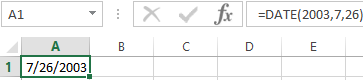
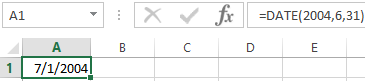
If you point a larger number for the «Day» argument (than the number of days in the pointed month), you receive the extra days, will be passed to the next month. For example, specifying 32 days for December, we will receive as a result on January 1.
The example of using the function:
Let’s set more days for June:
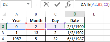
Examples of using the cell references as arguments:
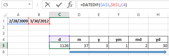
The DATEDIF function in Excel
It returns the difference between two dates.
The arguments:
- start date;
- final date;
- the code indicating to the units of counting (days, months, years, etc.).
The methods of measuring intervals between the given dates:
- to display the result in days — «d»;
- in months – «m»;
- in years – «y»;
- in months without years – «ym»;
- in days without months and years – «md»;
- in days without years – «yd».
In some versions of Excel, if you use the last two arguments («md», «yd»), the function may give an error. It is better to use to alternative formulas.
The examples of the operation the DATEDIF function:
In Excel 2007 version, this function is not in the directory, but it works. But you need to check the results are better, because there are flaws possible.
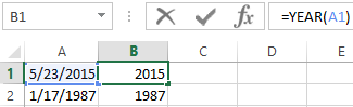
The YEAR function in Excel
It returns the year as an integer number (from 1900 to 9999), what corresponds to the specified date. There is only one argument must be entered in the structure of the function – is the date in a numerical format. The argument must be entered using the DATE function or represents to the result of evaluating other formulas.
The example of using the YEAR function:
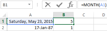
The MONTH function in Excel: the example
It returns the month as an integer number (from 1 to 12) for a date is specified in a numeric format. The argument – is the date of the month that you want to show in a numerical format. The dates in the text format this function does not handle correctly.
The examples of using the MONTH function:
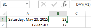
The examples of DAY, WEEKDAY and functions WEEKNUM in Excel
It returns the day as an integer number (from 1 to 31) for a date specified in a numeric format. The argument – it is the date of the day you want to find in a numerical format.
For returning of the weekday ordinal of the specified date, you can apply the function WEEKDAY:
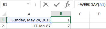
By default, the function considers Sunday the 1-st day of the week.
To display of the ordinal number of the week for the pointed date, you should use the WEEKNUM function:
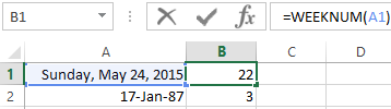
The date of 24. 05. 2015 is 22 week in a year. The week starts on Sunday (by default).
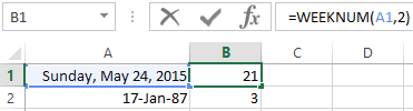
As the second argument the figure 2 is specified. Therefore, the formula considers that the week starts on Monday (the 2-d day of the week).
Download all examples functions for working with dates
For indicating of the current date, the function TODAY (no arguments) is used. To display the current time and date, the function NOW() is used.
The DATE function is a financial analyst’s best pal and categorized as a Date/Time function in Excel. The criticality of the DATE function’s role is sourced from Excel’s reluctance to keep the day, month, and year as a date. Instead, Excel stores them as a serial number.
Directly handing over dates as a text string may not work well for all Excel functions. So, we will supply the dates as a serial number using the DATE function to ensure that Excel and our worksheet formulas understand the instructions properly.

Syntax
The syntax of Excel Date function is as follows:
=DATE(year, month, day)
Arguments:
year – This is a required argument that represents the year component in the date. Enter it as a 4 digit number; entering a single digit will result in Excel automatically adding 1900 to it.
For example, entering year as ’10’ will instruct the formula to interpret the year argument as ‘1910’.
Excel refers to your computer’s date system set up to interpret the Year argument. Note that entering a negative value or a value greater than 9999 will return a #NUM! error.
month – This is a required argument that represents the month component in the date. Ideally, it must be an integer from 1 to 12 (January to December).
Alternatively, if you input a number greater than 12, Excel will count that many months starting from January of the year specified in the year argument. For example, entering year as 2001 and month as 18 will return a serial number that represents June 01, 2002. Note that Excel will return the date as the first date of the interpreted month (June 01 in our case), regardless of what you input in the date argument.
On the other hand, if you enter a value less than 1, Excel will reduce that many months from January of the year specified, plus 1. For example, if you enter month as -10 and year as 2001, Excel will return a serial number that represents February 01, 2000.
day – This is a required argument that represents the day component of the date. While in an ideal case, you will enter an integer from 1 to 31 as the date argument, it can be supplied as any other positive or negative integer and Excel will apply the same principles to compute the date as it does for the month argument.
Important characteristics of the DATE function
- DATE function returns a #NUM! error when
yearargument is supplied with a negative number or a number greater than 9999. - DATE function returns a #VALUE! error when any of its three arguments is supplied with a non-numeric value.
- If you see the Excel DATE function is returning a serial number like 36557 instead of a date, you will need to change the cell’s format. To do this, select the cell containing the returned date and search for the ‘Short Date’ option in the drop-down menu of cell formatting options in the ‘Number group’. These options sit on Excel’s Home Tab that appears at the top left.
Examples of the DATE function
Now let’s have a look at some of the examples of the DATE function in Excel.
Example 1 – The Plain – Vanilla DATE formula
In its purest form, this is what a DATE formula looks like:
=DATE(2001, 3, 15)

This formula returns a serial number that corresponds to the date March 15, 2001.
However, the formula can be slightly tweaked to incorporate the TODAY function encapsulated inside the YEAR function in Excel as well, like so:
=DATE(YEAR(TODAY()), 3, 15)

This formula will fetch the serial number for the current year (and the specified month and day), and return 03/15/2021.
Much the same way, you can use the TODAY function for the month argument as well, like so:
=DATE(YEAR(TODAY()), MONTH(TODAY()), 15)

This formula will fetch the serial number for the current year as well as the current month (and the specified day), and return 02/15/2021.
Example 2 – Using Cell References in DATE function Arguments
If the values you want to supply in the arguments are stored in cells on your spreadsheet, you can reference those cells, like so:
=DATE(A2, B2, C2)

With the values supplied from column A, the DATE function returns 04/30/2001.
Example 3 – Converting a number into a date using the DATE function
Let’s say you scalped the internet and landed on a large data set with dates written in a format that Excel does not understand (for example, 20052005).
In that (or similar) case, we can use the following formula to help Excel make sense of the data and interpret these numbers appropriately as dates:
=DATE(RIGHT(A2, 4), MID(A2, 3, 2), LEFT(A2, 2))

Recommended Reading: Excel MID Function
Addition and Subtraction of Dates With DATE function
We discussed earlier how Excel store dates as serial numbers. There is of course a logical reason why Excel does this – it enables us to add or subtract a specified number of days from a given date.
To illustrate how this works, we plugged the following formula into our sheet:
=DATE(2001, 3, 15) + 20

When you add a +20 at the end of this DATE formula, Excel will return the date 20 days after 03/15/2001, which is 04/04/2001.
Alternatively, to subtract a certain number of days, all you need to do is use a minus sign, like so:
=DATE(2001, 3, 15) - 10

But, let’s say you want to compute the number of days between today and another date. In that case, we will subtract both dates, like so:
=TODAY() - DATE(2021, 2, 20)

The formula will return the number of days between today (whenever that may be) and March 15, 2001.
Changing DATE format With DATE function
So, you added some neat formulas to your Excel sheet and everything worked out fine. But, let’s say you want to use different separators for the days (for example, ‘/’ instead of ‘-‘), or you want to use the name of the month instead of a number (for example, January instead of 01).
We discussed earlier that Excel will refer to your computer’s date format and uses the same format for displaying dates in a worksheet.
To change this format, you do not need a formula. Instead, you need to tweak some settings.
Select the cell that contains the output from the DATE function. Right-click, and choose «Format Cells». You should see the following dialogue box:

Choose the format of your preference and click «OK».
Conditional Formatting with DATE function
Let’s say you have a large data set and you want to separate the data points occurring before and after a certain date.
To do this, we will use Excel’s conditional formatting rules and instruct Excel to shade these 2 cells with 2 separate colors so it becomes easy for us to discern.
We have our dates listed out in column A, and we want to shade the dates occurring before 12/31/2012 in green, and the ones occurring after in red.
To illustrate the entire process, we will use the following formula as a starting point:
=$A2 < DATE(2012, 12, 31)

Notice how this formula returns a Boolean value but does not shade any cells.
Let’s move a step further and apply a shade.
Select the range A2:A8 and navigate to the «Conditional Formatting» drop-down menu in the «Styles» group under the «Home» tab, and select «Manage Rules»:

On the «Conditional Formatting Rules Manager» click the «New Rule» button.

After clicking on the «New Rule» you will see a list of Rule Types. Scroll over to «Use a formula to determine which cells to format» and choosing it will reveal a formula box. In this box, plug in the formula we used to fetch Boolean values and select the desired formatting, like so:

Click «OK» and you should return to the Conditional Formatting Rules Manager dialog box.
To shade the dates occurring after 12/21/2012 red, we will add another rule following the same process. The only difference, obviously, will be in the formula. Instead of using a ‘<‘, we will use a ‘>=’, like so: =$A2>=DATE(2012,12,31)

This is what the Rules Manager box should look like at this point. Make sure that the «Applies to» box contains the appropriate range.

As your final step, click on «Apply» and watch your date list switch colors.

I hope the guide gives you a confidence boost the next time you use DATE formulas in your worksheet. Remember, practice is key. By the time you are done practicing, we will have another Excel function for you to explore.
The Excel DATE function is a DATE & TIME function. This function returns the DATE value in numerical format. Convert the output to date format via using Format cell option.
In this article, we will learn how to use the DATE function in Excel.
Syntax of DATE Function:
year : valid numerical value for year
month : numerical value for month, can have zero and negative values
day : numerical value for day, can have zero and negative values
Example of DATE Function
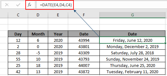
All of these might be confusing to understand. So, let’s test this formula via running it on the example shown below. So, here I have a table of some data. The first column contains the numeric values for the day value, second column contains month value and third contains the year value for the real date value as result.
Use the formula:

It will return 43994. Here all the arguments to the DATE function are given using cell reference. As you can see the value is not in date format. So for that just change the format of the result cell to short or long date format as required.
As shown in the above gif that you can change the format of any cell to any format using the format cell option. Now You can copy the formula from one to the remaining cells using the Ctrl + D shortcut key or using the drag down option in excel.
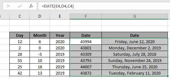
As you can see from the above snapshot that DATE function takes day, month and year value as input and returns the whole date value. Negative or zero value as argument returns the date shifting respectively as per value.
Excel DATE function : DATE function with other formulas to return result in date format. DATE function is mostly used with other logic functions for calculating date values in Excel. From one date value extract month, day and year for more calculation like the one shown below to get the next anniversary date.
Use the formula:
=DATE (YEAR (D5) + 1, MONTH(D5) , DAY(D5))
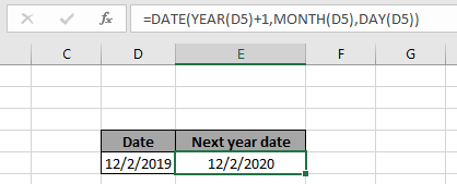
Here the day function extract day , Month function extracts month and year function extracts year value from the date and perform operation over numerical values and return the arguments to the DATE function to return required date value.
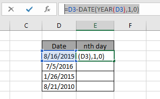
Get nth day from date of year in Excel
Here we have some random date values and we need to find the nth day of year from the date value.
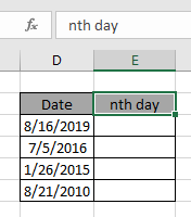
Use the formula:
= D3 — DATE ( YEAR ( D3 ) , 1 , 0 )
Explanation:
- YEAR function returns the year value of the given date.
- DATE function takes the argument and returns the last date of the previous year.
- The subtraction operator takes the difference of the two and returns the elapsed date.
Use the above function formulas to get the days between dates in Excel.
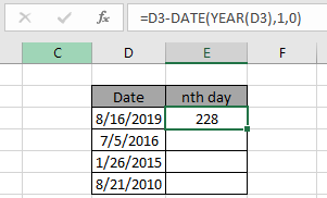
As you can see the formula works fine as it returns 228 as result. Now use drag drop down till the dataset dates.
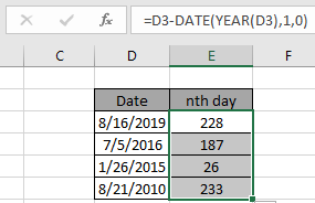
Here are the days from the date of the year calculated using the formula.
We can calculate the same result using one more logic. If we subtract the given date value from the first date of the same year and add 1 ( +1 ).
Generic formula:
= date — DATE ( YEAR ( date ) , 1 , 1 ) + 1
You can use any of the formulas as both return the same result.
Note: DO NOT give the date argument directly to the formula as Excel formula doesn’t necessarily understand the date value and returns error. Provide the date argument using the DATE function or using the cell reference option.
EDATE function example
Here we have a list of dates of birth with Emp ID.
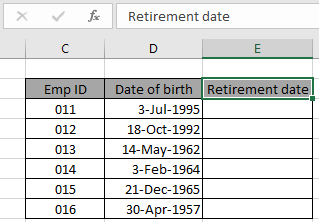
Here we need to find the retirement date from the given DAte of birth values.
Use the formula in E3 cell:

Here the date value is given as cell reference. Press Enter to get the retirement date.
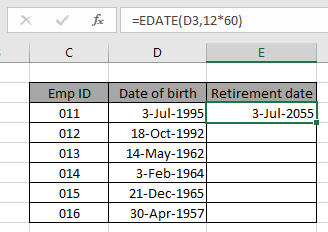
As you can see the retirement date for the 011 Emp ID comes out to be July 3rd, 2055. Now copy the formula in other cells using the drag down option or using the shortcut key Ctrl + D as shown below.
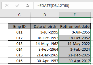
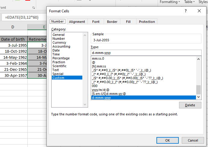
As you can see we obtained all employees’ retirement age using the Excel EDATE function. Generally the returned date value is not in the required date format. Use the format cell option or Ctrl + 1 as shown in the below snapshot.
Here are some observational notes shown below.
Notes:
- The formula only works with numbers.
- Arguments to the function must be numeric values or else the function returns #NAME? Error.
- No argument to the function returns #NUM! Error.
- Only No year argument returns the year value as 1900.
- MONTH and DAY arguments can be zero or negative. As day argument 1 returns 1st date of month, 0 input will return the just before date value from the previous month.
Hope this article about How to use the DATE function in Excel is explanatory. Find more articles on DATE & TIME formulas here. If you liked our blogs, share it with your fristarts on Facebook. And also you can follow us on Twitter and Facebook. We would love to hear from you, do let us know how we can improve, complement or innovate our work and make it better for you. Write to us at info@exceltip.com.
Related Article
How to calculate age from date of birth | returns the year age as numerical value from the date value comparing it with today’s date value.
SUM if date is between | Returns the SUM of values between given dates or period in excel.
Sum if date is greater than given date | Returns the SUM of values after the given date or period in excel.
2 Ways to Sum by Month in Excel | Returns the SUM of values within a given specific month in excel.
Popular Articles:
50 Excel Shortcuts to Increase Your Productivity | Get faster at your task. These 50 shortcuts will make you work even faster on Excel.
How to use the VLOOKUP Function in Excel | This is one of the most used and popular functions of excel that is used to lookup value from different ranges and sheets.
How to use the COUNTIF function in Excel 2016 | Count values with conditions using this amazing function. You don’t need to filter your data to count specific values. Countif function is essential to prepare your dashboard.
How to Use SUMIF Function in Excel | This is another dashboard essential function. This helps you sum up values on specific conditions.
So I’ve been battling with this issue all day.
Basically I have it now sorted and part of the solution was a code that Excel itself generated which is:
[$-en-AU]yyyy-mm-dd hh:mm
So, in the first instance,
- in a new spreadsheet, type your entry in as per usual, eg:
2026-01-31 10:00 - set the format of the cell to «custom» and use the above formula, ie
[$-en-AU]yyyy-mm-dd hh:mm - Hit enter and Bob’s your uncle!
Then save it as a CSV file, then close it and re-open it to check Excel hasn’t changed the date format.
The weird thing is if it does work (and I’ve re-tried it a few times successfully), when you check the format of the cell you’ve created, it’s changed the format to «General».
But seriously who cares. As long as it works!!
You can then copy and paste the cell and use it wherever you want!!
I hope this solution works for you!!
Regards
Richard