
Convert text data into numeric values
Updated on November 12, 2019
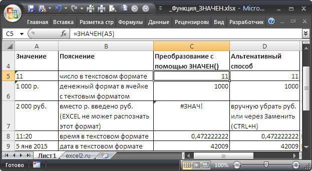
The VALUE function in Excel is used to convert numbers that have been entered as text data into numeric values so that the data may be used in calculations.
The information in this article applies to Excel versions 2019, 2016, 2013, 2010, and Excel for Mac.
SUM and AVERAGE and Text Data
Screenshot
Excel automatically converts problem data of this sort to numbers, so the VALUE function is not required. However, if the data is not in a format that Excel recognizes, the data can be left as text. When this situation occurs, certain functions, such as SUM or AVERAGE, ignore the data in these cells and calculation errors occur.
For example, in row 5 in the image above, the SUM function is used to total the data in rows 3 and 4 in columns A and B with these results:
- The data in cells A3 and A4 is entered as text. The SUM function in cell A5 ignores this data and returns a result of zero.
- In cells B3 and B4, the VALUE function converts the data in A3 and A4 into numbers. The SUM function in cell B5 returns a result of 55 (30 + 25).
The Default Alignment of Data in Excel
Text data aligns on the left in a cell. Numbers and dates align on the right.
In the example, the data in A3 and A4 align on the left side of the cell because it was entered as text. In cells B2 and B3, the data was converted to numerical data using the VALUE function and aligns on the right.
The VALUE Function’s Syntax and Arguments
A function’s syntax refers to the layout of the function and includes the function’s name, brackets, and arguments.
The syntax for the VALUE function is:
Text (required) is the data to be converted to a number. The argument can contain:
- The actual data enclosed in quotation marks. See row 2 of the example above.
- A cell reference to the location of the text data in the worksheet. See row 3 of the example.
#VALUE! Error
If the data entered as the Text argument cannot be interpreted as a number, Excel returns the #VALUE! error as shown in row 9 of the example.
Convert the Text Data to Numbers With the VALUE Function
Listed below are the steps used to enter the VALUE function B3 in the example above using the function’s dialog box.
Alternatively, the complete function =VALUE(B3) can be typed manually into the worksheet cell.
- Select cell B3 to make it the active cell.
- Select the Formulas tab.
- Choose Text to open the function drop-down list.
- Select VALUE in the list to bring up the function’s dialog box.
- In the dialog box, select the Text line.
- Select cell A3 in the spreadsheet.
- Select OK to complete the function and return to the worksheet.
- The number 30 appears in cell B3. It is aligned on the right side of the cell to indicate it is now a value that can be used in calculations.
- Select cell E1 to display the complete function =VALUE(B3) in the formula bar above the worksheet.
Convert Dates and Times
The VALUE function can also be used to convert dates and times to numbers.
Although dates and times are stored as numbers in Excel and there is no need to convert them before using them in calculations, changing the data’s format can make it easier to understand the result.
Excel stores dates and times as sequential numbers or serial numbers. Each day the number increases by one. Partial days are entered as fractions of a day — such as 0.5 for half a day (12 hours) as shown in row 8 above.
Thanks for letting us know!
Get the Latest Tech News Delivered Every Day
Subscribe
Содержание
- Свойство Range.Value (Excel)
- Синтаксис
- Параметры
- Замечания
- Пример
- Поддержка и обратная связь
- Как исправить Excel #Value! Ошибка —
- The Excel VALUE Function
- Function Description
- Value Function Examples
- Value Function Error
- Функция ЗНАЧЕН() в EXCEL
- Синтаксис функции
- Функции SUMIF, COUNTIF и COUNTBLANK возвращают значение «#VALUE!» Ошибка
- Симптомы
- Причина
- Обходной путь
- Примеры
- СУММЕСЛИ
- СЧЁТЕСЛИ
- COUNTBLANK
- Статус
- Дополнительные сведения
- Ссылка
Свойство Range.Value (Excel)
Возвращает или задает значение Variant , представляющее значение указанного диапазона.
Синтаксис
expression. Value (RangeValueDataType)
выражение: переменная, представляющая объект Range.
Параметры
| Имя | Обязательный или необязательный | Тип данных | Описание |
|---|---|---|---|
| RangeValueDataType | Необязательный | Variant | Тип данных значения диапазона. Может быть константой XlRangeValueDataType . |
Замечания
При задании диапазона ячеек с содержимым XML-файла электронной таблицы используются только значения первого листа в книге. Невозможно задать или получить несогласительный диапазон ячеек в формате электронной таблицы XML.
Элемент range по умолчанию переадресовывает вызовы значения value без параметров. Таким образом, someRange = someOtherRange эквивалентно someRange.Value = someOtherRange.Value .
Для диапазонов, первая область которых содержит несколько ячеек, значение возвращает значение Variant , содержащее двухмерный массив значений в отдельных ячейках первого диапазона.
При назначении массива размером 2 тумм для свойства Value значения будут скопированы в диапазон за одну операцию. Если целевой диапазон больше массива, остальные ячейки получат значение ошибки.
Назначение массива диапазону с несколькими областями не поддерживается должным образом, и его следует избегать.
Пример
В этом примере для ячейки A1 на листе 1 активной книги задается значение 3,14159.
В этом примере выполняется цикл по ячейкам A1:D10 на листе 1 активной книги. Если одна из ячеек имеет значение меньше 0,001, код заменяет значение на 0 (ноль).
В этом примере выполняется цикл над значениями в диапазоне A1:CC5000 на Листе1. Если одно из значений меньше 0,001, код заменяет значение на 0 (ноль). Наконец, он копирует значения в исходный диапазон.
Поддержка и обратная связь
Есть вопросы или отзывы, касающиеся Office VBA или этой статьи? Руководство по другим способам получения поддержки и отправки отзывов см. в статье Поддержка Office VBA и обратная связь.
Источник
Как исправить Excel #Value! Ошибка —
#Значение! error — это очень общее сообщение об ошибке, которое может быть сложным и разочаровывающим при поиске источника. Это полностью зависит от сложности формулы, которая генерирует сообщение об ошибке. Думать о #Значение! ошибка вроде этого: «Эй! Ваша формула введена неправильно, или вы передаете неверный аргумент своей формуле, и я не знаю, что делать сейчас ». Расплывчато, верно? Ну вы пришли в нужное место!
Есть много общих проблем, которые могут привести к #Значение! ошибка, и все они должны быть обработаны по-разному.
Пробелы и текст
Часто при создании первоклассных документов мы срываемся или защемляем наши клавиатуры в отчаянии. Иногда пальцы бегут от нас и вводят значения в скрытых неизвестных глубинах Excel. Много раз, #Значение! ошибки возникают из-за того, что значения хранятся в виде текста, когда они должны быть числовыми. Пробелы, безусловно, не позволят вещам работать. Это разные способы проверки таких вещей.
- Если вы знаете ячейки, на которые ссылается ваша формула, тогда вы можете использовать «Найти и заменить»
- Выделите ячейки, на которые ссылается ваша формула.
- На вкладке «Главная страница» нажмите «Найти и выбрать»> «Заменить». Или нажмите Ctrl + F в Windows или CMD + F в MAC.
- Убедитесь, что курсор находится в поле «Найти что», и нажмите пробел один раз. Затем нажмите «Заменить все»
- После завершения вы увидите, что расстояние между 2 и 5 в столбце цены становится $ 300,25, а #Значение! ошибка уходит.

# Значение ошибки не устранено с помощью SUM и вычитания

И теперь ошибка исчезает.

Иногда вы получите значения, которые хранятся в виде текста случайно. Вы увидите маленький красный треугольник ошибок в углу ячейки. Когда вы наведете на него курсор, вы увидите, что на нем написано «Число, хранящееся как текст». Если это вызывает проблему с вашей формулой, просто выберите «Преобразовать в число», и это должно решить вашу проблему.

Другие формулы, которые могут вызвать #Значение! ошибки — это формулы вычитания, ссылки на формулы и формулы запроса. Убедитесь, что у вас нет неправильного интервала, синтаксиса, ссылок или аргументов.
Другие способы справиться с #Value! ошибки
Иногда ошибку не так просто понять, как другие. Возможно, у вас сложная формула или вы ссылаетесь на другие листы, используя формулу, и не можете видеть все одновременно. Вы можете попробовать следующее решение, чтобы помочь вам разобраться в проблеме.
- Выберите ячейку, показывающую #Значение! Ошибка и выберите «Показать шаги расчета».
- Вы получите всплывающее окно, которое поможет вам оценить вашу формулу. Когда коробка открыта, посмотрите информацию, представленную в поле «оценка:». Подчеркнутые элементы станут первой частью формулы, которая будет оценена. Если у вас есть простая формула, подобная показанной, у нее, скорее всего, будет только один шаг для оценки.

Иногда при просмотре этапов расчета будет показан результат формулы. Нажмите «Оценить» и перезапустите. Это покажет вам формулу с самого начала.


Как только вы выясните сообщение об ошибке и узнаете, откуда возникла проблема, вы можете просто исправить ее и продолжить работу над проектом.
Хотя это не всегда рекомендуется, вы можете использовать функцию IFERROR () для обработки #Значение! Сообщение об ошибке. Функция IFERROR () в основном говорит: «Если есть ошибка, пропустите это и« сделайте это ». В приведенном ниже примере вы увидите, что мы хотим видеть слово «Ошибка» в случае ошибки. Есть много способов справиться и использовать это, хотя важно понять, что на самом деле делает IFERROR (). Зачастую это затруднит заметить или увидеть, что у вас есть проблема где-то в вашей книге, и часто может усложнить ошибки отслеживания.
Функция IFERROR () также будет обрабатывать и другие ошибки, такие как #NA, #REF и некоторые другие. Лучше всего использовать эту функцию только в случае необходимости или если вы ожидаете, что подобные вещи произойдут.
Просто «оберните» IFERROR () вокруг всей формулы, как показано.
Источник
The Excel VALUE Function
Excel stores values as either text or numeric values, so, for example, if you attempt to use the text value «10» in an addition, multiplication, or other numeric operation, you will get an error.
Therefore, if you want to extract a numeric value from a text string, you need to convert this to a number, before Excel will be able to recognise it as a numeric value. The Value function can be used to do this.
Function Description
The Excel VALUE Function converts a text string into a numeric value.
The syntax of the function is:
where the text argument is a text string that can be translated into a number. This may be presented in any of the numeric, date or time formats that are recognised by Excel.
Value Function Examples
The following spreadsheet shows five examples of the Value function, used to convert five different text string representations of numbers into numeric values.
| A | |
|---|---|
| 1 | =VALUE( «50» ) |
| 2 | =VALUE( «1.0E-07» ) |
| 3 | =VALUE( «5,000» ) |
| 4 | =VALUE( «20%» ) |
| 5 | =VALUE( «12:00:00» ) |
| A | |
|---|---|
| 1 | 50 |
| 2 | 0.0000001 |
| 3 | 5000 |
| 4 | 0.2 |
| 5 | 0.5 |
The examples above show how the Excel Value function successfully interprets the different formats of numbers. For example,
- In cell B2, the function understands the text value «1.0E-07» to represent the scientific notation for the number 0.0000001;
- In cell B3, the function understands the text value «5,000» to represent the number 5000;
- In cell B4, the function understands the text value «20%» to represent the number 0.2;
- In cell B5, the function converts the text representation of the time «12:00:00» to the value 0.5. This is the underlying value that Excel uses to represent the time 12:00:00. If cell B5 were formatted as a time this would display the time 12:00:00.
See the Microsoft Office website for further details and examples of the Excel Value function.
Value Function Error
If you get an error from the Excel Value function, this is most likely to be the #VALUE! error:
Источник
Функция ЗНАЧЕН() в EXCEL
history 28 мая 2014 г.
Функция ЗНАЧЕН () возвращает число (если преобразование текстовой строки прошло удачно) или ошибку #ЗНАЧ! (если преобразование не удалось).
Синтаксис функции
ЗНАЧЕН(текст)
Текст — Текст (текстовая строка) в кавычках или ссылка на ячейку, содержащую текст, который нужно преобразовать.
- Текст может быть в любом формате, допускаемом в Microsoft Excel для числа, даты или времени (см. ниже). Если текст не соответствует ни одному из этих форматов, то функция возвращает значение ошибки #ЗНАЧ!
- Обычно функцию ЗНАЧЕН () не требуется использовать в формулах, поскольку необходимые преобразования значений выполняются в Microsoft Excel автоматически. Эта функция предназначена для обеспечения совместимости с другими программами электронных таблиц.
В файле примера приведены разные варианты преобразований текстовых строк.
Как правило это числа, даты и время введенные в ячейки с текстовым форматом. При вводе этих значений в ячейки с форматом Общий проблем не возникает и преобразование происходит автоматически (функция ЗНАЧЕН () не нужна).
Функция ЗНАЧЕН () может потребоваться при преобразовании чисел из текстового формата, когда эти числа возвращаются функциями ЛЕВСИМВ() , ПСТР() и др. Но, в этом случае альтернативой может служить операция сложения с нулем. Например, формула =ЗНАЧЕН(ЛЕВСИМВ(«101 Далматинец»;3)) аналогична формуле =ЛЕВСИМВ(«101 Далматинец»;3)+0 ( подробнее здесь ).
Источник
Функции SUMIF, COUNTIF и COUNTBLANK возвращают значение «#VALUE!» Ошибка
Симптомы
Формула, содержащая функции SUMIF, SUMIFS, COUNTIF, COUNTIFS или COUNTBLANK , может возвращать ошибку #VALUE!» в Microsoft Excel.
Это поведение также применяется к Dfunctions, таким как DAVERAGE, DCOUNT, DCOUNTA, DGET, DMAX, DMIN, DPRODUCT, DSTDEV, DSTDEVP, DSUM, DVAR и DVARP. Функции OFFSET и INDIRECT также имеют такое поведение.
Причина
Это происходит, когда формула, содержащая функцию, ссылается на ячейки в закрытой книге и ячейки вычисляются.
Если открыть указанную книгу, формула будет работать правильно.
Обходной путь
Чтобы обойти это поведение, используйте сочетание функций SUM и IF в формуле массива.
Примеры
Необходимо ввести каждую формулу в виде формулы массива. Чтобы ввести формулу массива в Microsoft Excel для Windows, нажмите клавиши CTRL+SHIFT+ВВОД.
СУММЕСЛИ
Вместо того чтобы использовать формулу, аналогичную следующей:
Используйте следующую формулу:
СЧЁТЕСЛИ
Вместо того чтобы использовать формулу, аналогичную следующей:
используйте следующую формулу:
COUNTBLANK
Вместо того чтобы использовать формулу, аналогичную следующей:
используйте следующую формулу:
Когда следует использовать формулу массива SUM(IF()), используйте логическое И или ИЛИ, чтобы заменить функцию СУММЕСЛИМЕСЛИ или СЧЁТЕСЛИМЕСЛИ.
Статус
Такое поведение является особенностью данного продукта.
Дополнительные сведения
Функция СУММЕСЛИ использует следующий синтаксис:
Ссылка
Для получения дополнительных сведений о мастере, который может помочь вам создать эти функции, щелкните справку Microsoft Excel в меню справки, введите суммирование значений, соответствующих условиям, с помощью мастера условной суммы в помощнике office или мастере ответов, а затем нажмите кнопку «Поиск», чтобы просмотреть раздел.
Для получения дополнительных сведений о формулах массива щелкните » Справка Microsoft Excel» в меню «Справка», введите сведения об использовании формул для вычисления значений на других листах и книгах в помощнике Office или мастере ответов, а затем нажмите кнопку «Поиск», чтобы просмотреть раздел.
Источник
Функция ЗНАЧЕН преобразует текстовый аргумент в число.
Описание функции ЗНАЧЕН
Преобразует строку текста, отображающую число, в число.
Синтаксис
=ЗНАЧЕН(текст)Аргументы
текст
Обязательный. Текст в кавычках или ссылка на ячейку, содержащую текст, который нужно преобразовать.
Замечания
- Текст может быть в любом формате, допускаемом в Microsoft Excel для числа, даты или времени. Если текст не соответствует ни одному из этих форматов, то функция ЗНАЧЕН возвращает значение ошибки #ЗНАЧ!.
- Обычно функцию ЗНАЧЕН не требуется использовать в формулах, поскольку необходимые преобразования значений выполняются в Microsoft Excel автоматически. Эта функция предназначена для обеспечения совместимости с другими программами электронных таблиц.
Пример
The VALUE function is a text function that converts a number from text format to numerical format where data is in an Excel-recognized format such as date, currency, time, etc. Mostly, if Excel recognizes a number, it automatically converts the data into numerical format. However, in other cases, we can do so using the VALUE function.
The VALUE function is most helpful when we seek compatibility with other spreadsheet programs and for using the numerical text resulting from text functions in calculations.

Syntax
The syntax of the VALUE function is quite straightforward and is given below.
=VALUE(text)
Arguments:
The VALUE function accepts only one argument, and it is mandatory.
‘text‘– This mandatory argument contains the value in text format that needs to be converted. The value of the text argument can be passed as a direct value in double quotes or as a cell reference.
Important Characteristics of the VALUE Function
Some noteworthy features of the VALUE function are as follows.
- The VALUE function only accepts the value that is recognized by Microsoft Excel such as constant number, locale formatted number, date, or time. If the value of the text argument is any value that is not recognized by Excel, the function results in a #VALUE! error.
- If the value of the text argument is empty, the VALUE function returns zero.
When using the VALUE function, it is important to note the alignment of the data as left-aligned data indicates text format whereas right-aligned data is number format.
Examples of VALUE Function
There are instances when the given data which looks like a number cannot be used further for calculations and analysis. In such scenarios, the VALUE function comes in very handy. Below are some examples to provide a better understanding of the function.
Example 1 – Simple Use of VALUE Function
In this example, we will use different types of input values for the text argument to better understand the functionality of the VALUE function.
We have taken time, date, date and time together, number in text format, and percentage as the input values. The function used is as follows.
=VALUE(B3)

In the first example, the value of the text argument is a time value which upon conversion to numerical format is transformed into the serial number. Excel stores time as fractions of a day. The VALUE function simply converted the time format to an actual serial number which can further be used in formulas.
The next example is in date format and like the time data, the VALUE function converts the date value to a sequential number as stored in Excel. The third example is a combination of date and time, and the VALUE function returns the expected result of the corresponding serial number and fraction of both date and time in cell C5.
The fourth example is a text which looks like a number. If we wish to use the data in cell B6 for any calculations, the result will also take on the text format. With the help of the VALUE function, the number is transformed from text format to numerical format.
The last example is a percentage value. The VALUE function returns the calculated numerical value of the percentage which is 0.25 in this case.
Now that the basic functionality of the VALUE function is clear, check some useful applications of the same in the examples below.
Example 2 – Converting String to Number using VALUE Function
In this scenario, we collected small donations from our neighbors to get essentials for the homeless shelter. The data collected was user-generated hence it is in text format.

To calculate the total donations received, we can extract the dollar amount and then sum it up. To segregate the donation amount from the given text, we will use the TEXTBEFORE function. It will extract the characters that occur before the dollar sign ($), which is the amount in this case. The formula used is as follows.
=TEXTBEFORE(B3,"$")
Now that the donation amount is segregated in column C, the total donation can be calculated.

Unfortunately, all the extracted data in column C is text, which is clear due to its left alignment, since the TEXTBEFORE function is a text function. Therefore, the total sum couldn’t be downloaded as seen in cell C10. To rectify this, we will use the VALUE function to convert all the data in column C into the numeric format and then calculate the total donation received. The updated formula to be used is as follows.
=VALUE(TEXTBEFORE(B3,"$"))

We can combine everything in one formula as follows.
=SUM(VALUE(TEXTBEFORE(B3:B8,"$")))

Note: One can also use the LEFT function in place of the TEXTBEFORE function to achieve the same result.
Example 3 – Converting Currency to Numerical Format
Here, in this case, we have received the monthly sales for the last year. As the sales report is from the India office, the currency formatting is different where a comma is used as a group separator in hundreds, thousands, and so on. Excel does not recognize the formatting, so it treats the sales numbers as text.

To be able to use the data for further calculations, we wish to convert them from text format to number format. As it is not an Excel-recognized format, the VALUE function will return a #VALUE! error.

To overcome this, we can first use the SUBSTITUTE function to replace all the commas with an empty string and then use the VALUE function. The formula used will be as follows.
=SUBSTITUTE(C3,",","")

Now the sales values in column D are in a recognizable format i.e. text, with the help of the VALUE function, we can convert the same in number format. Combining both steps, the final formula used will be as follows.
=VALUE(SUBSTITUTE(C3,",",""))

As evident by the right alignment of the data in column D, all the sales values are now in a number format and therefore can be further used for calculations.
Example 4 – Converting Time using the VALUE Function
In this example, we are conducting an online test where the completion time is set to 10:00 AM. However, every applicant can take extra time up to 20 minutes, but points will be assigned depending on the extra time taken which will eventually be deducted from the actual score. Here are the points to be deducted as per the completion time.

As the first step, we will calculate the extra time taken in each case. The formula used will be as follows.
=B4-$C$2

Now that we have all the values in column C, we can use the nested IF function to compare the time as per the point system and then assign the corresponding points. However, while using the delayed time data from C4:C7, we will wrap it in the VALUE function to ensure that Excel treats the time value as a number and not text.
The logic used will be as follows.
If the delayed time (C4) is less than 5 minutes, then assign 1 point, else if the delayed time is less than 10 minutes, assign 2 points….) and so on till 20 minutes. If no condition is met, the formula returns FALSE.
The formula used will be as follows.
=IF(C4<VALUE("0:05"),1,IF(C4<VALUE("0:10"),2,IF(C4<VALUE("0:15"),3,IF(C4<VALUE("0:20"),4))))

Now we have the final points that will be deducted from the final score in each case. With the help of the VALUE function, we were able to convert the time value from minutes to numerical format and execute the nested IF function.
VALUE Function vs NUMBERVALUE Function
Both the VALUE and NUMBERVALUE functions convert text that looks like a number from text format to numerical format but the NUMBERVALUE function transforms the data using the given group and decimal separators which help the function understand the format.
If the data is not in an Excel-recognized format, the VALUE function returns a #VALUE! error whereas with the NUMBERVALUE function, we can mention the group and decimal separator used in the data to convert it. Let’s understand it better using an example.

The data in cell B4 is a currency value in euros and is in a text format. The VALUE function does not recognize the data and hence throws a #VALUE! error whereas the NUMBERVALUE function converts the data from text to number format due to the mentioned decimal and group separator.
VALUE Function vs VALUETOTEXT Function
Now we know that the VALUE function converts text that looks like a number from the text format to numerical format. The VALUETOTEXT function performs the opposite conversion. The VALUETOTEXT function converts a value to text format depending on the concise or strict format.
Hopefully, now you have a clear idea about how to use the VALUE function to your advantage. Practice and discover new applications of the said function.
Функция Excel VALUE
Функция Excel VALUE помогает преобразовать текстовую строку, представляющую число (например, число, формат даты или времени) в число.

Синтаксис
=VALUE(text)
Аргумент
Текст (Обязательно): текст, который нужно преобразовать в число. Это может быть:
- Текст в кавычках;
- Или ссылку на ячейку, содержащую текст.
Возвращаемое значение
Числовое значение.
Функция Примечание
- #СТОИМОСТЬ! Ошибка возникает, если текст не является форматом числа, даты или времени, распознаваемым Microsoft Excel;
- Поскольку Excel автоматически преобразует текст в числовые значения по мере необходимости, обычно функция ЗНАЧЕНИЕ не требуется.
Пример
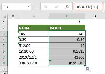
Как показано на скриншоте ниже, мы собираемся преобразовать список текстовой строки в числа. Функция VALUE может помочь в достижении этого.
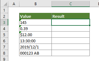
Выберите пустую ячейку, скопируйте в нее приведенную ниже формулу и затем перетащите маркер заполнения, чтобы применить формулу к другим ячейкам.
=VALUE(B3)
Связанные функции
Функция ПОДСТАВИТЬ в Excel
Функция ЗАМЕНА в Excel заменяет текст или символы в текстовой строке другим текстом или символами.
Функция Excel TEXT
Функция ТЕКСТ преобразует значение в текст с заданным форматом в Excel.
Функция Excel TEXTJOIN
Функция Excel TEXTJOIN объединяет несколько значений из строки, столбца или диапазона ячеек с определенным разделителем.
Функция Excel TRIM
Функция Excel TRIM удаляет все лишние пробелы из текстовой строки и сохраняет только отдельные пробелы между словами.
Функция ВЕРХНИЙ в Excel
Функция Excel ВЕРХНИЙ преобразует все буквы заданного текста в верхний регистр.
Лучшие инструменты для работы в офисе
Kutools for Excel — Помогает вам выделиться из толпы
Хотите быстро и качественно выполнять свою повседневную работу? Kutools for Excel предлагает 300 мощных расширенных функций (объединение книг, суммирование по цвету, разделение содержимого ячеек, преобразование даты и т. д.) и экономит для вас 80 % времени.
- Разработан для 1500 рабочих сценариев, помогает решить 80% проблем с Excel.
- Уменьшите количество нажатий на клавиатуру и мышь каждый день, избавьтесь от усталости глаз и рук.
- Станьте экспертом по Excel за 3 минуты. Больше не нужно запоминать какие-либо болезненные формулы и коды VBA.
- 30-дневная неограниченная бесплатная пробная версия. 60-дневная гарантия возврата денег. Бесплатное обновление и поддержка 2 года.
")
Вкладка Office — включение чтения и редактирования с вкладками в Microsoft Office (включая Excel)
- Одна секунда для переключения между десятками открытых документов!
- Уменьшите количество щелчков мышью на сотни каждый день, попрощайтесь с рукой мыши.
- Повышает вашу продуктивность на 50% при просмотре и редактировании нескольких документов.
- Добавляет эффективные вкладки в Office (включая Excel), точно так же, как Chrome, Firefox и новый Internet Explorer.
")
Комментарии (0)
Оценок пока нет. Оцените первым!

| Раздел функций | Текстовые |
| Название на английском | VALUE |
| Волатильность | Не волатильная |
| Похожие функции | ДАТАЗНАЧ |
| Похожие процедуры | Числа как текст – в настоящие числа |
Что делает эта функция?
Эта функция преобразует фрагмент текста, который похож на число, в фактическое число.
Если число в середине длинного фрагмента текста, его нужно будет извлечь, используя другие текстовые функции, такие как ПОИСК, ПСТР, НАЙТИ, ЗАМЕНИТЬ, ЛЕВСИМВ, ПРАВСИМВ.
Синтаксис
=ЗНАЧЕН(Текст)
Форматирование
Специального форматирования не требуется.
Результат будет показан в виде числового значения на основе исходного текста.
Если знак % включен в текст, результатом будет десятичная дробь, которая может затем быть отформатирована в процентах.
Если исходный текстовый формат отображается как время чч:мм, результатом будет время.
То же самое применимо для других форматов.
Пример применения функции
Извлечь количество процентов из текста сложно, не зная заранее, сколько в нем знаков. Это может быть от 1 цифры (5%) до 4 цифр с запятой (12,25%).
Единственный способ определить процентное значение – это факт, что оно всегда заканчивается знаком %. Невозможно определить начало значения, за исключением того, что ему предшествует пробел.
Основная проблема заключается в расчете длины числа для его извлечения.
Если при извлечении предположить максимальную длину из четырех цифр и знака %, когда процент только одна цифра, при обычном извлечении по маске “?????%” в выражение попадут буквы.
Чтобы обойти проблему, можно использовать функцию ПОДСТАВИТЬ, чтобы увеличить количество пробелов между словами в тексте. Теперь при извлечении по маске “?????%” любые лишние символы будут пробелами, которые функция ЗНАЧЕН проигнорирует.

Формула ниже аналогична формуле на картинке и извлечет из ячейки A1 проценты длиной от 1 до 5 знаков, включая запятую:
=ЗНАЧЕН(ПСТР(" "&ПОДСТАВИТЬ(A1;" ";" ");ПОИСК("?????%";" "&ПОДСТАВИТЬ(A1;" ";" "));6))
Файл с примерами
Ниже интерактивный файл с примерами.
Двойным кликом по ячейке с формулой можно ее просмотреть, скопировать или отредактировать. Также есть ссылка для скачивания файла.
|
Ни где не могу найти, что означает (смысл) .Value, например Range.Value. Нигде найти не могу, а везде применяется |
|
|
CAT Пользователь Сообщений: 49 |
Value — значение какого-либо элемента. А так если не знаешь, то в перв. очередь глянь в обычный англ-рус словарь. Дальше по смыслу можно понять, куда прикручивается то или иное свойство и зачем. |
|
air Пользователь Сообщений: 90 |
Если не знаете VBA настолько, что не знаете смысл Value, то, наверное, надо бы что-нибудь обобщенное про VBA почитать. Например по ссылкам, предложенным на этом сайте (здесь есть свойство Value: http://msoffice.nm.ru/vba/range.htm) . |
|
слэн  Пользователь Сообщений: 5192 |
#4 24.11.2008 15:53:07 value — это имя процедуры, осуществляющей доступ к свойству объекта для ячейки — возвращает значение — число или текст. если в ячейке введена формула, то это ее значение, иначе — это значение, введенное пользователем с учетом преобразования при вводе.( т.е ввод значения — нажатие enter, tab или с помощью галочки в строке формул — это тоже вызов процедуры доступа к свойству ячейки) Живи и дай жить.. |