
#VALUE is Excel’s way of saying, «There’s something wrong with the way your formula is typed. Or, there’s something wrong with the cells you are referencing.» The error is very general, and it can be hard to find the exact cause of it. The information on this page shows common problems and solutions for the error.
Use the drop-down below or jump to one of the other areas:
-
Problems with subtraction
-
Problems with spaces and text
-
Other solutions to try
Fix the error for a specific function
Don’t see your function in this list? Try the other solutions listed below.

Problems with subtraction
If you’re new to Excel, you might be typing a formula for subtraction incorrectly. Here are two ways to do it:
Subtract a cell reference from another
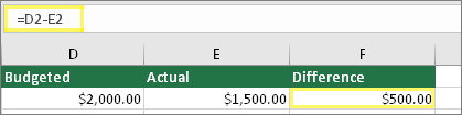
Type two values in two separate cells. In a third cell, subtract one cell reference from the other. In this example, cell D2 has the budgeted amount, and cell E2 has the actual amount. F2 has the formula =D2-E2.
Or, use SUM with positive and negative numbers
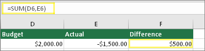
Type a positive value in one cell, and a negative value in another. In a third cell, use the SUM function to add the two cells together. In this example, cell D6 has the budgeted amount, and cell E6 has the actual amount as a negative number. F6 has the formula =SUM(D6,E6).
If you’re using Windows, you might get the #VALUE! error when doing even the most basic subtraction formula. The following might solve your problem:
-
First do a quick test. In a new workbook, type a 2 in cell A1. Type a 4 in cell B1. Then in C1 type this formula =B1-A1. If you get the #VALUE! error, go to the next step. If you don’t get the error, try other solutions on this page.
-
In Windows, open your Region control panel.
-
Windows 10: Click Start, type Region, and then click the Region control panel.
-
Windows 8: At the Start screen, type Region, click Settings, and then click Region.
-
Windows 7: Click Start and then type Region, and then click Region and language.
-
-
On the Formats tab, click Additional settings.
-
Look for the List separator. If the List separator is set to the minus sign, change it to something else. For example, a comma is a common list separator. The semicolon is also common. However, another list separator might be more appropriate for your particular region.
-
Click OK.
-
Open your workbook. If a cell contains a #VALUE! error, double-click to edit it.
-
If there are commas where there should be minus signs for subtraction, change them to minus signs.
-
Press ENTER.
-
Repeat this process for other cells that have the error.
Subtract a cell reference from another
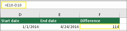
Type two dates in two separate cells. In a third cell, subtract one cell reference from the other. In this example, cell D10 has the start date, and cell E10 has the End date. F10 has the formula =E10-D10.
Or, use the DATEDIF function
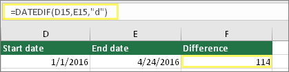
Type two dates in two separate cells. In a third cell, use the DATEDIF function to find the difference in dates. For more information on the DATEDIF function, see Calculate the difference between two dates.
Make your date column wider. If your date is aligned to the right, then it’s a date. But if it’s aligned to the left, this means the date isn’t really a date. It’s text. And Excel won’t recognize text as a date. Here are some solutions that can help this problem.
Check for leading spaces
-
Double-click a date that is being used in a subtraction formula.
-
Put your cursor at the beginning and see if you can select one or more spaces. Here’s what a selected space looks like at the beginning of a cell:

If your cell has this problem, proceed to the next step. If you don’t see one or more spaces, go to the next section on checking your computer’s date settings.
-
Select the column that contains the date by clicking its column header.
-
Click Data > Text to Columns.
-
Click Next twice.
-
On Step 3 of 3 of the wizard, under Column data format, click Date.
-
Choose a date format, and then click Finish.
-
Repeat this process for other columns to ensure they don’t contain leading spaces before dates.

Check your computer’s date settings
Excel uses your computer’s date system. If a cell’s date isn’t entered using the same date system, then Excel won’t recognize it as a true date.
For example, let’s say that your computer displays dates as mm/dd/yyyy. If you typed a date like that in a cell, Excel would recognize it as a date and you’d be able to use it in a subtraction formula. However, if you typed a date like dd/mm/yy, then Excel wouldn’t recognize that as a date. Instead, it would treat it as text.
There are two solutions to this problem: You could change the date system that your computer uses to match the date system you want to type in Excel. Or, in Excel you could create a new column and use the DATE function to create a true date based on the date stored as text. Here’s how to do that assuming your computers date system is mm/dd/yyy and your text date is 31/12/2017 in cell A1:
-
Create a formula like this: =DATE(RIGHT(A1,4),MID(A1,4,2),LEFT(A1,2))
-
The result would be 12/31/2017.
-
If you want the format to appear like dd/mm/yy, press CTRL+1 (or
+ 1 on the Mac). -
Choose a different locale that uses the dd/mm/yy format, for example, English (United Kingdom). When you’re done applying the format, the result would be 31/12/2017 and it would be a true date, not a text date.
 + 1 on the Mac).
Note: The formula above is written with the DATE, RIGHT, MID, and LEFT functions. Please notice that it is written with an assumption that the text date has two characters for days, two characters for months, and four characters for year. You may need to customize the formula to suit your date.
Problems with spaces and text
Often #VALUE! occurs because your formula refers to other cells that contain spaces, or even trickier: hidden spaces. These spaces can make a cell look blank, when in fact they are not blank.
1. Select referenced cells
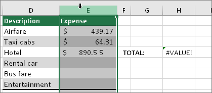
Find cells that your formula is referencing and select them. In many cases removing spaces for an entire column is a good practice because you can replace more than one space at a time. In this example, clicking the E selects the entire column.
2. Find and replace

On the Home tab, click Find & Select > Replace.
3. Replace spaces with nothing
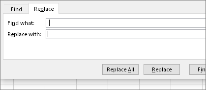
In the Find what box, type a single space. Then, in the Replace with box, delete anything that might be there.
4. Replace or Replace all
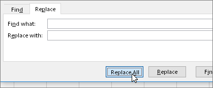
If you are confident that all spaces in the column should be removed, click Replace All. If you’d like to step through and replace spaces with nothing on an individual basis, you can click Find next first, and then click Replace when you are confident the space isn’t needed. When you’re done, the #VALUE! error may be resolved. If not, go to the next step.
5. Turn on the filter
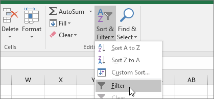
Sometimes there are hidden characters other than spaces that can make a cell appear blank, when it’s not really blank. Single apostrophes within a cell can do this. To get rid of these characters in a column, turn on the filter by going to Home > Sort & Filter > Filter.
6. Set the filter

Click the filter arrow  , and then deselect Select all. Then, select the Blanks checkbox.
7. Select any unnamed checkboxes
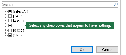
Select any check boxes that don’t have anything next to them, like this one.
8. Select blank cells, and delete

When Excel brings back the blank cells, select them. Then press the Delete key. This will clear any hidden characters in the cells.
9. Clear the filter
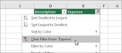
Click the filter arrow , and then click Clear filter from… so that all cells are visible.
10. Result
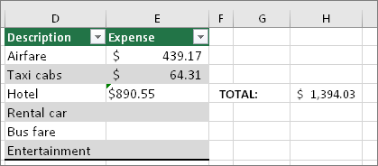
If spaces were the culprit of your #VALUE! error then hopefully your error has been replaced by the formula result, as shown here in our example. If not, repeat this process for other cells that your formula refers to. Or, try other solutions on this page.
Note: In this example, notice that cell E4 has a green triangle and the number is aligned to the left. This means the number is stored as text. This may cause more problems later. If you see this problem, we recommend converting numbers stored as text to numbers.
Text or special characters within a cell can cause the #VALUE! error. But sometimes it’s hard to see which cells have these problems. Solution: Use the ISTEXT function to inspect cells. Please note that ISTEXT doesn’t resolve the error, it simply finds cells that might be causing the error.
Example with #VALUE!
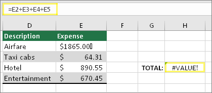
Here’s an example of a formula that has a #VALUE! error. This is likely due to cell E2. There is a special character that appears as a small box after «00.» Or as the next picture shows, you could use the ISTEXT function in a separate column to check for text.
Same example, with ISTEXT
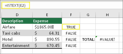
Here the ISTEXT function was added in column F. All cells are fine except the one with the value of TRUE. This means cell E2 has text. To resolve this, you could delete the cell’s contents and retype the value of 1865.00. Or you could also use the CLEAN function to clean out characters, or use the REPLACE function to replace special characters with other values.
After using CLEAN or REPLACE, you’ll want to copy the result, and use Home > Paste > Paste Special > Values. You might also have to convert numbers stored as text to numbers.
Formulas with math operations like + and * may not be able to calculate cells that contain text or spaces. In this case, try using a function instead. Functions will often ignore text values and calculate everything as numbers, eliminating the #VALUE! error. For example, instead of =A2+B2+C2, type =SUM(A2:C2). Or, instead of =A2*B2, type =PRODUCT(A2,B2).
Other solutions to try
Select the error

First select the cell with the #VALUE! error.
Click Formulas > Evaluate Formula
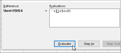
Click Formulas > Evaluate Formula > Evaluate. Excel will step through the parts of the formula individually. In this case the formula =E2+E3+E4+E5 breaks because of a hidden space in cell E2. You can’t see the space by looking at cell E2. However, you can see it here. It shows as » «.
Sometimes you just want to replace the #VALUE! error with something else like your own text, a zero or a blank cell. In this case you can add the IFERROR function to your formula. IFERROR will check to see if there’s an error, and if so, replace it with another value of your choice. If there isn’t an error, your original formula will be calculated. IFERROR will only work in Excel 2007 and later. For earlier versions you can use IF(ISERROR()).
Warning: IFERROR will hide all errors, not just the #VALUE! error. Hiding errors isn’t recommended because an error is often a sign that something needs to be fixed, not hidden. We don’t recommend using this function unless you are absolutely certain your formula works the way that you want.
Cell with #VALUE!
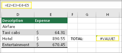
Here’s an example of a formula that has a #VALUE! error due to a hidden space in cell E2.
Error hidden by IFERROR
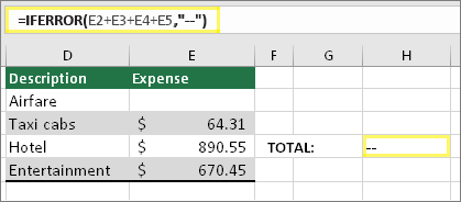
And here’s the same formula with IFERROR added to the formula. You can read the formula as: «Calculate the formula, but if there’s any kind of error, replace it with two dashes.» Note that you could also use «» to display nothing instead of two dashes. Or you could substitute your own text, such as: «Total Error».
Unfortunately, you can see that IFERROR doesn’t actually resolve the error, it simply hides it. So be certain that hiding the error is better than fixing it.
Your data connection may have become unavailable at some point. To fix this, restore the data connection, or consider importing the data if possible. If you don’t have access to the connection, ask the creator of the workbook to make a new file for you. The new file ideally would only have values, and no connections. They can do this by copying all the cells, and pasting only as values. To paste as only values, they can click Home > Paste > Paste Special > Values. This eliminates all formulas and connections, and therefore would also remove any #VALUE! errors.
See Also
Overview of formulas in Excel
How to avoid broken formulas
No matter how good you’re with Excel and formulas, sometimes you will end up getting a few error here and there.
And the #VALUE error is one of the common errors you’re likely to come across.
Excel returns the #VALUE! Error when there is something wrong with the cells you are referencing in a formula or the way you typed the formula.
The #VALUE! error is very general, so it may take some work and digging around to identify its cause.
This tutorial describes possible causes of the #VALUE! error in Excel and explains some techniques for fixing the error.
Understanding #VALUE Error in Excel
If you have worked with Excel formulas, I am sure you have been greeted by the #VALUE error already.
In most cases, this happens when the formula expects you to give it a specific type of data, but your input doesn’t match that expectation.
Don’t worry!
Let’s break down why the #VALUE error occurs in your worksheet and what you can do to fix it.
There are a few common reasons for the #VALUE error:
- Incorrect Data Type: If you use the incorrect data type in a formula, you’ll likely encounter this error. For example, when trying to sum a text value instead of a number.
- Missing Values: If a referenced cell is empty or contains an unexpected value, Excel might not know how to process it, causing the error.
- Special Characters: Some formulas are sensitive to special characters. If special characters are present in a cell, they can trigger the #VALUE error.
Imagine you’re trying to calculate a total price by multiplying the number of items with the unit price, but the unit price cell contains a mixture of numbers and text.
Your formula would return a #VALUE error because Excel doesn’t know how to multiply numbers with text.
Fixing the error can often be as simple as correcting the input data or changing the formula itself.
For example, by removing any text or special characters in the cell containing the unit price, your formula can work as intended.
Also read: #NUM! Error in Excel – How to Fix it?
Causes of #VALUE! Error and How to Fix It
Now that you have a good understanding of what is a VALUE error in Excel, let me show you what causes these value errors (using some examples) and how you can easily fix them.
Cause #1: Using Text Strings in Formulas that Expect Number Arguments
Some formulas in Excel, for example, the addition arithmetic formula, are designed to work with number values; therefore, if you supply them with text values, the formulas return #VALUE! error instead of a total.
Let’s consider the following frequency table with a text value in cell B3 instead of a number value.
An absentminded data entry clerk may have entered the text value.

We want to determine the total frequency using an addition arithmetic formula.
We use the steps below:
- Select cell B5 and type in the formula below:
=B2+B3+B4

- Press Enter.

The formula returns a #VALUE! error instead of a total because one of the operands in cell B3 is a text string and not an expected number value.
The arithmetic formula only works with numeric values.
How to Fix
We can use the following techniques to fix the #VALUE! error caused by text string arguments in a formula where number values are expected:
- Delete the text string from the target cell range so that only numeric values that can be added remain, as shown in the example below.

- Replace the text value with the correct number value, as shown in the example below, where we replaced “fifteen” in cell B3 with “15.”

- Use the Excel built-in functions instead of arithmetic operators. Generally, the built-in functions are designed to disregard data types unsupported by the function.
In this example, we use the SUM function to add all the numbers in the target cell range instead of the arithmetic formula:

Notice that the SUM function has disregarded the text value in cell B3 and added only the numeric values in the cell range B2:B4.
Some Important Things to Know
- A space character in the target cell range can also trigger the #VALUE! error when you use the arithmetic formula, as seen in the below example:

The cell with the space character appears blank, but when you select it and check in the formula bar, you find it has a space character represented by an apostrophe.
The space character causes the #VALUE! error because Excel considers it a text string. You can fix this error by deleting all space characters in the target cell range.
- Sometimes, you may accidentally enter a space between numbers, which can trigger a #VALUE! error as shown in the example below:

Notice a space between 9 and 5 in the value in cell A2. The space makes the value a text string, not a number causing the error.
You can fix the error by removing the space between 9 and 5 in cell A2:

- Sometimes, you may accidentally enter a mix of digits and letters in a cell, and this causes the #VALUE! error as seen in the example below:

Notice that in cell A2, instead of entering a nine followed by a zero, someone entered a nine followed by the letter “O.”
The value looks like a numeric value, ninety, but it is not; it is a text string causing the #VALUE! error. You can fix the error by replacing the letter “O” with a zero (0).

Also read: #NAME? Error in Excel – How to Fix!
Cause #2: Entering a Formula Incorrectly
If you mistype an arithmetic formula, Excel will return the #VALUE! Error as shown in the below example:

You notice that the arithmetic formula in cell C2 is intended to compute the difference between the values in cells A2 and B2 and has a comma instead of a minus symbol between the operands.
You can fix the error by typing the formula correctly with a minus symbol between the values:

How to Get Help in Finding the Correct Syntax of a Formula
If you do not know the correct syntax of a formula in Excel, you can consult Excel’s built-in help feature:
Use Excel’s Built-in Help Feature
- Type an equal sign symbol in a cell to start a formula.
- Begin typing the name of the function you want to use, for example, AVERAGE. When the full name of the function appears in the IntelliSense drop-down as below, press the tab key to select the function:

- Press Ctrl + A to open the Function Arguments dialog box.

The Function Arguments dialog box displays the syntax of the function you want to use and explains each argument.
You can use this information to enter the formula correctly.
When dealing with complex formulas, it can be challenging to identify the cause of the value error. In cases like that, it is recommended that you select a segment of the formula and press the F9 key to calculate and return the output of that segment. This process allows you to troubleshoot the formula in parts.
Cause #3: Unsupported Date Formats
Excel supports many date formats, but sometimes you work with datasets with dates in formats not recognized by Excel.
In that case, Excel treats the dates in unsupported formats as text strings. Therefore, if you use such dates in date functions, Excel returns the #VALUE! error.
Let’s consider the dataset below with dates in cells A4, A5, and A7 that are in formats not recognized by Excel:

When we apply the YEAR function in column B to return the years of the dates in column A, we get the #VALUE! error in cells B4, B5, and B7:

The only way to fix this error caused by unsupported date formats is to ensure the dates are in formats recognized by Excel.
Note: Dates in Excel are serial numbers where each day is assigned a unique number starting from January 1, 1900, which is assigned the value 1.
Therefore one way to test whether a date is in a format recognized by Excel is to select an empty cell and enter a formula that adds the value 1 to the date, as shown below.

If the formula returns a date, then the date is in a format supported by Excel.
Otherwise, the date is in a format not recognized by Excel, and you need need to reenter the date in a format supported by Excel.
Suppressing the #VALUE! Error (using IFERROR or ISERROR)
Another way of fixing the #VALUE! error is using the IF and ISERROR functions to suppress the error and display an informative message instead.
Let’s consider the following dataset.

We want to use a formula to add the days in column B to the dates in column A and show the result in column C. The formula suppresses the #VALUE! error if it occurs and displays an informative message instead.
We use the following steps:
- Select cell C2 and enter the below formula:
=IF(ISERROR(A2+B2),"Correct the date",A2+B2)

- Drag or double-click the fill handle feature to copy the formula down the column.

Explanation of the formula
=IF(ISERROR(A2+B2),”Correct the date”,A2+B2)
The formula checks whether the result of the calculation of adding days in column B to dates in column A is a #VALUE! error or not.
Suppose the output is a #VALUE! error, the formula returns the second argument, “Correct the date.” Otherwise, it returns the result of the calculation.
Note: If you are using a newer version of Excel, you can use the IFERROR function instead of combining IF and ISERROR functions. However, remember that the IFERROR function catches many other errors besides the #VALUE! error, for example, the #REF! and #DIV/0! errors.
Some Tips for Preventing #VALUE Errors
Below are some useful tips you can use in your day-to-day work to avoid the value error in Excel
1. Check for text or special characters: When using formulas that expect numeric values, ensure that only numeric values are used (as text or special characters can cause this error). If you’re using a cell reference, make sure it contains a numerical value and not text.
2. Use appropriate functions: Instead of using mathematical operations, use functions like SUM(), COUNT(), or AVERAGE() to handle your calculations. For example, if you have a cell containing text and a cell containing a number, instead of using =A1+A2, use SUM(A1:A2), which will ignore any non-numeric values.
3. Check formula syntax: Double-check your formula for any missing or extra characters which could be causing the error. Verify that you’ve constructed the syntax correctly. For example, ensure your nested IF functions are properly formatted.
4. Use Excel Table format: Consider converting your data to an Excel Table format, making it easier to work with and reducing the chance of errors. To convert data into an Excel Table, press Ctrl + T or use the Format as Table button on the Home tab.
With these tips, you can prevent Excel’s #VALUE errors and make your work more efficient and error-free.
How to Filter Cells With #VALUE! Error
If auditing a workbook, you should filter the cells with the #VALUE! errors so that you can quickly find and fix them.
Suppose we have the dataset below with the #VALUE! errors in cell C4, C5, and C7.

We want to filter the cells with the #VALUE! errors.
This can be done using the following steps:
- Select the cell range C1:C7 with the errors.

- On the Data tab, click the Filter button on the Sort & Filter group.

- Click the Filter button in cell C1 and deselect all options in the bottom area of the drop-down except the #VALUE! option and click OK.

All the cells with the #VALUE! errors are filtered, and you can fix the errors one by one.

This tutorial described various causes of the #VALUE! error in Excel and gave possible solutions. We hope you found the tutorial helpful.
Other Excel articles you may also like:
- SPILL Error in Excel – How to Fix?
- How to Turn Off Error Sound in Excel?
- Subscript Out of Range Error in VBA – How to Fix!
- How to Calculate Standard Error in Excel?
What is #Value! Error in Excel?
Error is a common and integral part of Excel formulas and functions, but fixing those errors is what makes you a pro in Excel. As a beginner, finding those errors and restoring them to work correctly is not easy. Every error occurs only because of a user’s mistakes. So, it is essential to know our mistakes and why those errors are happening. In this article, we will show you why we get #VALUE! Errors in Excel and how to fix them.
For example, the simple formula may return as the #VALUE! Error if a space character in any cell is created to clear a cell. To fix the error, the cell which contains a space character needs to be selected and then pressed the Delete key.
Table of contents
- What is #Value! Error in Excel?
- How to Fix #Value! Error in Excel?
- Case #1
- Case #2
- Example
- Case #3
- Example
- Things to Remember Here
- Recommended Articles
- How to Fix #Value! Error in Excel?
How to Fix #Value! Error in Excel?
You can download this Error Value Excel Template here – Error Value Excel Template
Case #1
#VALUE!: This excel errorErrors in excel are common and often occur at times of applying formulas. The list of nine most common excel errors are — #DIV/0, #N/A, #NAME?, #NULL!, #NUM!, #REF!, #VALUE!, #####, Circular Reference.read more occurs for multiple reasons depending upon the formula we use. The most common reason for this error is the wrong data type used in the cell references.
Follow the below steps to fix the value error in Excel.
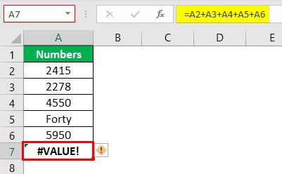
- Look at the below formula for adding different cell values.

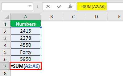
In the above basic Excel formula, we are trying to add numbers from A2 to A6 in cell A7, and we have got the result of #VALUE! Error. In cell A5, we have a value as “Forty,” which is the wrong data type, so it returns #VALUE! - To get the correct sum of these numbers, we can use the SUM function in excel.

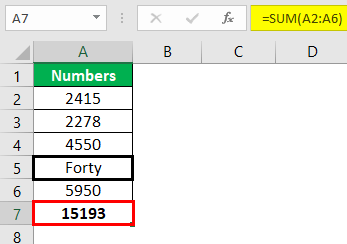
- We get the following result.

The SUM function has ignored the wrong data type in cell A5, adding the remaining cell values and giving the total. - Otherwise, we can change the text value in cell A5 to get the correct result.

For the earlier formula, we have only changed the A5 cell value to 4,000. So now, our previous function is working properly.

Case #2
Now, we will see the second case of #VALUE! Error in Excel formulas.
Example
- Look at the below formula.
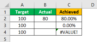
We have divided column B with column A. And we have got three different results.
- Result 1 says B2/A2. In both cells, we have numerical values, and the result is 80%.
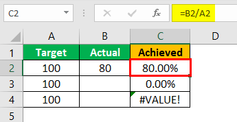
- Result 2 says B3/A3. Since there is no value in cell B3, we have got the result of 0%.
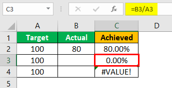
- Result 3 says B4/A4. It is also the same case as Result 2.
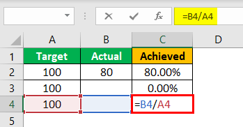
- We have got an #VALUE! Error, so curious case.
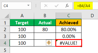
- The main reason for this error is that the empty cell is not truly blank because there could be an errant space character.
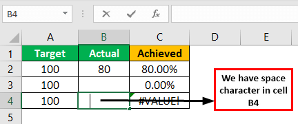
In cell B4, we have a space character that is not visible to naked eyes. However, it is the reason why we have got #VALUE! Error.
We can use the LEN Excel FunctionThe Len function returns the length of a given string. It calculates the number of characters in a given string as input. It is a text function in Excel as well as an inbuilt function that can be accessed by typing =LEN( and entering a string as input.read more or ISBLANK Excel function to deal with these unnoticeable space characters.
- LEN function will give the number of characters in the selected cell. LEN considers a space character as a single character.
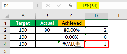
Look at the above function. We have got one character resulting in cell B4, which confirms B4 cell is not an empty cell.
- Similarly, the ISBLANK function shows TRUE if the cell is empty. Otherwise, it shows FALSE.
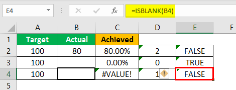
Look at the above result. We have got FALSE as a result for the B4 cell. So, we can conclude that cell B4 is not an empty cell.
Case #3
Another case of resulting #VALUE! Excel error is because the function argument data type is wrongly stored.
Example
Look at the below image.
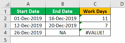
- In the above formula example, we have used the NETWORKDAYS Excel functionThe NETWORKDAYS function is a date and time function that determines the number of working days between two given dates and is widely used in the fields of finance and accounting. When calculating the working days, NETWORKDAYS automatically excludes the weekend (Saturday and Sunday).read more to find the actual working days between two dates.
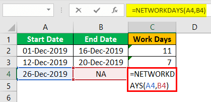
- The first two cells got the result, but we have an error result of #VALUE!
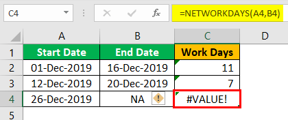
The end date in the B4 cell has the value of NA, the non-date value, resulting in #VALUE!
- We need to enter the proper date value in cell B3 to correct this error.

There is also another chance of getting the same error even though we have the date value.
- For example, look at the below cell.
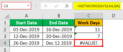
Even though we have a date in cell B4, we still have the #VALUE! Error. In cell C4, a date is not a date stored as a text value, so we need to convert this to a proper date format to get the correct result.
Things to Remember Here
- Other error values are explained in separate articles. This article is dedicated to #VALUE! Error.
- The #VALUE! Error occurs for multiple reasons. We have listed above all the possible scenarios of this error.
Recommended Articles
This article has been a guide to Excel #VALUE! Error. Here, we discuss fixing a value error in Excel with examples and a downloadable Excel template. You may learn more about excel from the following articles: –
- VLOOKUP Errors
- Excel Error Bars
- On Error Goto 0 in VBA
- On Error Resume Next in VBA
Excel doesn’t make mistakes, but you as a user, might. If you’ve entered a formula, and Excel can’t understand what one or more of the elements in the formula are trying to do, or if they are incorrectly entered, you’ll receive an error. The fix for each type of error is different.
In this article, we’ll walk you through how you can resolve the #VALUE! error, if you have one of those on your worksheet.

What is #VALUE! Error in Excel?
A #VALUE! error, as the name suggests, results when you erroneously enter an incorrect value in an Excel formula. The value could either be explicitly entered as an argument in the formula or supplied as a cell reference. However, fixing it just requires correctly inserting the value that you’ve added erroneously.
If you have a #VALUE! error on your sheet, we’re going to help you get rid of it in a couple of minutes. But before that, let’s talk about what causes a #VALUE! error.
Why Does it Appear?
A #VALUE! error occurs when one of the values supplied isn’t the value that the formula was expecting. For instance, leaving a referenced cell blank when the formula expected a value, or referencing to a cell that contains text when the formula expected a numeric value could both give you a #VALUE! error.
You can solve most Excel errors swimmingly, but there’s a caveat with the #VALUE! error. The thing is, some Excel functions automatically ignore inconsistent values. For instance, say cell B2 and B3 have the values 2 and «ABC», respectively. When you simply use an operator to add these values [i.e., =B2+B3], you’ll get a #VALUE! error.
However, if you use the SUM function [=SUM(B2:B3)], it will simply ignore the text string and return 2.
Examples
Let’s walk through a few formulas that could give you a #VALUE! error, and ways to fix it.
1. Number + Text
Adding a number to a text string is going to make Excel unhappy. If you’ve added a number and a text string, you’ll see a #VALUE! error on your worksheet. Let’s build upon the example we used in the previous section.

You have the number 2.49 in cell B2 and a text string «NA» in cell B3. You simply add an operator between cell references to get the total, like so:
=B2+B3
Naturally, you end up with a #VALUE error.
The fix here is simple. Just change the value in cell B3 to a number. For instance, changing the value in cell B3 to 3.99 solves the error, and the formula then returns 6.48.

Alternatively, you could use the SUM function, like so:
=SUM(B2:B3)

The SUM function will ignore any non-numeric values. Therefore, in this case, it will return 2.49.
2. Number + Space
This one can sometimes be tricky, especially if you have a large data set that has a lot of blank cells. If one of those cells has a space character, you’re going to pull your hair out finding that cell… unless you use a function like ISBLANK or LEN.
If your data set is indeed large with a lot of blank cells, just add a helper column next to it and apply the following formula to the entire column:
=ISBLANK(B2)

The formula will return TRUE for all cells that are actually empty, and FALSE if there’s a space character in any of those cells. In the example, notice how even though cell B3 looks blank, the ISBLANK function tells us that it has some value, which in all likelihood, is a space character.
So, circling back to the #VALUE! error and how it relates to a space character, it works pretty much the same way as the previous example. Instead of a text string, you’re now adding a space character to a numeric value, which Excel doesn’t understand.
Simply adding an arithmetic operator to add these values will return a #VALUE! error. However, again, the SUM function will work just fine. Alternatively, you could just remove the space character to make the formula with the arithmetic operator work.

3. Invalid argument value
If you’ve entered an inconsistent argument value in a formula, it will give you a #VALUE! error. For instance, say you’re trying to use the EOMONTH function. You have a column full of dates. So, you just apply the formula to the entire column, but a couple of them show #VALUE! errors.

Your inner Sherlock wants to dig a little and see what’s amiss. You find that a few of those columns have the employee’s last name instead of a date. Since the name of an employee is an incorrect argument to supply to the EOMONTH function, it returns a #VALUE! error.
Now, you don’t actually need to be Mr. Holmes to realize what will fix the problem. All you need to do is replace the employee’s name with a valid date.

If it didn’t resolve the error, read through the next example.
4. Dates formatted as text
When you enter a date, and you receive a #VALUE! error referencing it in a formula, check the cell formatting. Let’s take the last example and say we added a new employee to our list.
While trying to find the end of the first month you again run into a #VALUE! error.

The Joining date in this case looks like a valid date. Then what’s the problem?
The thing is, the dates have been imported from another file and are formatted as text. So the solution is simple – we just need to convert the text formatted date to an actual date that excel can recognize.
Now, there are a ton of ways you can convert text or numbers into dates, so look at our comprehensive tutorial on converting text and numbers to dates to correctly format your dates in a jiffy. Once you’ve done that, your #VALUE! error should disappear.

Alright, that’s all the ways you can kick the #VALUE! error out of your worksheet and make room for a valid output. While you get up to speed with these techniques, we’ve got something in the oven for you. When you’re done, you know where to find us.
When you’re working formulas in Excel, many times you will encounter the #VALUE error.
While the error is quite generic and doesn’t tell you what the problem is, in most cases, this happens when you give a formula a data type that is not expected (explained with examples below).
For example, if you have a few numbers that you’re adding in Excel, and you also try and add a text value in the same formula, Excel will give you an error. This is because Excel expects only numbers to be used in addition or subtraction.
While the easiest way to tackle the #VALUE error would be to make sure that the data types are correct in the formulas, it may not always be possible.
In this tutorial, I will show you a couple of methods you can use to get rid of the value error in Excel.
Value Error Becuase of Text String in Formulas
Some formulas are designed to only work with numbers.
And when there are non-numbers (such as text strings) used in the formula, you may see a value error.
In the image below is a very simple example where I need to add the scores of a student in different subjects.
While I have the numbers for all the subjects, I don’t have them for Math (and there is NA written instead of the score value).
If I use a simple arithmetic equation to get the sum of all the scores, I will get a value as shown below.

This is because the formula expects the only add numbers and I’m referencing a cell that has a text string instead.
How to tackle this?
In such simple addition subtraction formulas, one way to get rid of the error would be to remove the text string so that only numbers are left that can be added.
In our above example, if I remove the text ‘NA’ from the cell, the formula would work just fine.
Another way you can tackle this VALUE error is by using in-built functions instead of using the arithmetic equation.
Many of the commonly used Excel formulas are built in a way where they ignore any unexpected data type that is not supported by the formula.
For example, in this case, you can use the SUM formula, which would ignore all the text strings and only add the numbers.

Another possible reason that can give you a value error is when you have a space character in a cell that you have referenced in a formula. While most of the formulas are designed to ignore empty cells with space characters, in case you are using a simple arithmetic equation to add or subtract values, having a space character in a cell could give you a value error (as space character is considered a text string).
Value Error Because of Incorrect Argument Type in Formulas
If you’re using a formula that gives you a value error, there’s a good chance you have used an argument that is not the expected data type in the formula.
Let me give you an example and explain.
Below I have the year, month, and day value in three separate cells.
If I use this data in the DATE formula to get the serial number of this date, it is going to give me a value error.

This is because the date formula expects only numeric values as arguments, and in this formula, I have the month name which is a text string.
How to tackle this?
Check and double-check the formula to make sure that the argument types are correct.
It’s possible that you may be using formulas that you’re not very well versed with.
In such cases, it’s a good idea to check the help for each formula and make sure that the argument type is correct.
Pro Tip: Sometimes, the formulas can get large and complex and it could be difficult to find out what’s causing the error. A good technique in such cases to debug the formula would be to select a portion of the formula in the formula bar and hit the F9 key. The F9 key computes and gives you the result of the selected portion of the formula. This allows you to debug the Formula part-by-part.
Value Errors Due to Incorrect Date Format
Excel has multiple in-built date formats that it can recognize.
But in some cases, you may have a date in a format that Excel does not recognize as a date.
In such a scenario, Excel would treat those dates as text strings.
Now, if you try and use these dates in formulas that are built to handle date values, you will get a value error.
Let me explain with an example.
Below I have a date in cell A1, but this is not in the format that Excel recognizes as a proper date format.
If I try and use this date in the EOMONTH formula (which requires a date as one of the arguments). it will give me the value error.

How to tackle this?
The only way to tackle this issue is to make sure that the date is in the right format.
Pro tip: A quick trip to make sure that the date is in the right format is to go to an empty cell and add 1 to the date value. For example, if you have the date in cell A1, then you go to an empty cell and enter =A1+1. If you get a result, then the date is in the right format, and if you get an error, then it needs to be corrected
Removing #VALUE Error Using IF or IFERROR Functions
Excel has some built-in error handling formulas that can help you tackle the value error.
This can be done using the IFERROR formula (or a combination of IF and ISERROR).
Below I have a data set where I have the dates in column A and the number of days that I want to add to these dates in column B.

In column C, I use the below formula to get the date after the specified number of days for each date:
=A2+B2

As you can see, some of the results show the value error as the dates are not in the right format (i.e., these are in a format that Excel doesn’t recognize as a date, hence these are considered as text strings).
You can use the below formula to get a more meaningful text instead of the value error.
=IFERROR(A2+B2,"Check the date")

The above IFERROR formula would return the result of the first argument, and in case that results is an error, then it would return the second argument.
You can also achieve the same thing by using the below combination of IF and ISERROR formula
=IF(ISERROR(A2+B2),"Check the Date",A2+B2)
The above first checks whether the result of the calculation is an error or not. If it’s an error, it returns the second argument, else the third argument.
Note that if you’re using excel 2003 or versions prior to that, you would not have access to the IFERROR formula (as it was introduced from Excel 2007 onwards)
One drawback of using the IFERROR formula is that it is going to catch all the different types of error (be it #N/A or #DIV/0 #VALUE, #REF, etc.). So no matter what’s causing the error, IFERROR formula would bucket everything as an error and give you the specified second argument
Find All Cells with the #VALUE Error
If you’re auditing someone else’s work, it may be useful to know how to quickly find out all the cells that have the value error in them.
This can be done using a simple Find operation in Excel.
Below are the steps to quickly find out all the cells that contain the value error in a worksheet:
- Click the Home tab

- In the Editing group, click on Find and Select

- In the options from the drop-down, click on Find. This will open the Find and Replace dialog box
- Click on the Options button. This will make available some additional options

- In the Find and Replace dialog box, make the following changes:
- In the ‘Find what’ field, enter VALUE!
- From the ‘Within’ drop-down, select Workbook (or keep in Worksheet if you only want to find the error in the active worksheet)
- In the ‘Look in’ drop-down, select Values

- Click on Find All

The above steps would scan your entire worksheet (or workbook if you selected that) and give you a list of all the cells that contain the value error.
You should see the list of cells as shown below.

Now you can go through each of these cells one by one and handle these, or if you want to delete these or highlight these in one go, you can do that as well.
To select all the cells that have the value error, click on any of the listed cells in the Find and Replace dialog box, and then use the keyboard shortcut Control + A (hold the Control key and press the A key). If you’re using Mac, use Command + A instead.
That’s all that you need to know about the value error in Microsoft Excel.
In this tutorial, I covered the possible reasons that can cause the Value error and how to tackle these, some inbuilt error-handling formulas that you can use in case you get the value error, and how to quickly find and select all the cells that contain the value error in the worksheet or the workbook.
I hope you found this tutorial useful.
Other Excel tutorials you may also like:
- NAME Error in Excel (#NAME?)- What Causes it and How to Fix it!
- #REF! Error in Excel – How to Fix the Reference Error!
- How to Get Rid of #DIV/0! Error in Excel? Easy Formulas!
- Use IFERROR with VLOOKUP to Get Rid of #N/A Errors
- Identify Errors Using Excel Formula Debugging (2 Methods)
This article is all about the #VALUE! error in Excel and the different ways to fix it. We will also look at the reasons why we encounter a #VALUE! in Excel in this tutorial.
What is #VALUE! error?
A #VALUE! error is displayed in an Excel spreadsheet when a value or formula is not the expected type. You are seeing this error probably because you entered a text value instead of a number value in a formula or a number value for a date value in a formula.
When does the #VALUE! error occur?
The #VALUE! error occurs due to multiple causes. Let us look at the different instances when this occurs in Excel.
1. Summing text and numerical values together


You can see that a series of cells that include text, date, and numerical values were summed up manually in the cell below. On pressing ENTER on the keyboard, the #VALUE! error shows up.
This happens because Excel is looking for a set of numerical or date values only to add them together and give an answer based on that. Excel is unable to add the values together because of a text value in between.
Note that no #VALUE! error is displayed when you sum these values using the SUM function in Excel. The SUM function is smarter and automatically removes all text values in the calculation.
2. Summing text values

In the image above, we have summed up three text values in three different cells together. Again, we didn’t use the SUM function here, and instead, we summed each value manually putting a + sign in the middle. As a result, we see a #VALUE! error.
The reason is simple. Excel cannot sum text values together. If you had used the SUM function to sum these text values together, the result would be 0 because it didn’t find any summable values in any cell.
The result will be the same if you try to find the difference between these values and almost any mathematical function in Excel.

3. Multiplying numbers with text or blank cells

In this image above, we are trying to multiply a text value with a number and the result is a #VALUE! error on pressing ENTER. Similarly, if you try to multiply a number with a blank cell in Excel you get the #VALUE! error.

A blank cell denotes a cell with an unnecessary space in an empty cell. A space in between formulas also gives a #VALUE! error in Excel.
4. Summing and multiplying ranges


In this image, we are trying to sum and multiply the two ranges but we get the result as a #VALUE! error. The reason is that the SUM function cannot add and multiply two ranges at a time. You need to use the SUMPRODUCT formula for that.
The SUMPRODUCT formula multiplies the adjacent values of corresponding ranges and returns a sum of it. However, the trick is to make the SUM formula work without having to use the SUMPRODUCT function is to press CTRL+SHIFT+ENTER before finishing the formula.
5. Providing a text value to the NETWORKDAYS function


The NETWORKDAYS function is used to count the working days between two dates. In the example above, we have provided a text value with a date value for the function that is unable to count the days and is giving the result as a #VALUE! error.
6. Creating an illogical IF formula


You can see that we did not provide any appropriate logical text for the IF formula to give an appropriate true or false value. You see a #VALUE! error displaying on pressing ENTER.
Tips to fix the #VALUE! error for different cases
Here are the tips to fix #VALUE! error in Excel for different instances like these.
1. Summing text and numerical values together
When you sum numbers manually without using the SUM function, make sure to add numbers with numbers or date values only based on your preferences and date values with date values only to avoid getting the #VALUE! error.
2. Summing only text values
Excel cannot add or subtract text values and will display the #VALUE error when you sum, multiply or subtract them manually. However, to avoid getting the error, use built-in formulas like SUM, PRODUCT, SUMPRODUCT, etc. to let Excel ignore a text or any other values that cannot be quantified.
3. Multiplying numbers with text or blank cells
If you have a blank space in a cell where you are applying a formula that is showing a #VALUE! error. Make sure to remove all unnecessary spaces from cells while you are applying a formula to a set of values.
If the dataset is too large to be modified, consider using the TRIM function on your datasets to remove all extra spaces and mistakes from them.
4. Summing and multiplying ranges
You cannot normally sum and multiply two ranges using the SUM formula in Excel. To be able to sum and multiple ranges at the same time, you can use the SUMPRODUCT function to multiply the corresponding ranges and give a sum of them.
Or, press CTRL+SHIFT+ENTER before finishing the SUM formula to make it work like the SUMPRODUCT formula.
5. Providing a text value to the NETWORKDAYS function
The NETWORKDAYS function requires two date values to count the number of working days between them. Avoid entering text or numerical values and end getting a vague answer or the famous #VALUE error.

6. Creating an illogical IF formula
Make sure you provide the IF function with an appropriate logical test. Here’s is an example of a correct IF function.

Here, we are creating a condition that if the values in the range are less than 20, then display “Low” in the active cell, if not, display “High” in the active cell.

Note that we have changed the values to help you understand how an IF function works.
Read more about the IF function in detail here.
Conclusion
This article was all about the #VALUE! error in Excel and the different ways to fix it. Stay tuned for more amazing Excel tutorials like this only on QuickExcel!
References: ExcelJet.
The #VALUE! error appears when a value is not the expected type. This can occur when cells are left blank, when a function that is expecting a number is given a text value, and when dates are evaluated as text by Excel. Fixing a #VALUE! error is usually just a matter of entering the right kind of value.
The #VALUE error is a bit tricky because some functions automatically ignore invalid data. For example, the SUM function just ignores text values, but regular addition or subtraction with the plus (+) or minus (-) operator will return a #VALUE! error if any values are text.
The examples below show formulas that return the #VALUE error, along with options to resolve.
Example #1 — unexpected text value
In the example below, cell C3 contains the text «NA», and F2 returns the #VALUE! error:
=C3+C4 // returns #VALUE!

One option to fix is to enter the missing value in C3. The formula in F3 then works correctly:
=C3+C4 // returns 6

Another option in this case is to switch to the SUM function. The SUM function automatically ignores text values:
=SUM(C3,C4) // returns 4.5

Example #2 — errant space character(s)
Sometimes a cell with one or more errant space characters will throw a #VALUE! error, as seen in the screen below:

Notice C3 looks completely empty. However, if C3 is selected, it is possible to see the cursor sits just a bit to the right of a single space:

Excel returns the #VALUE! error because a space character is text, so it is actually just another case of Example #1 above. To fix this error, make sure the cell is empty by selecting the cell, and pressing the Delete key.
Note: if you have trouble determing whether a cell is truly empty or not, use the ISBLANK function or LEN function to test.
Example #3 — function argument not expected type
The #VALUE! error can also arise when function arguments are not expected types. In the example below, the NETWORKDAYS function is set up to calculate the number of workdays between two dates. In cell C3, «apple» is not a valid date, so the NETWORKDAYS function can’t compute working days and returns the #VALUE! error:

Below, when proper date is entered in C3, the formula works as expected:

Example #4 — dates stored as text
Sometimes a worksheet will contain dates that are invalid because they are stored as text. In the example below, the EDATE function is used to calculate an expiration date three months after a purchase date. The formula in C3 returns the #VALUE! error because the date in B3 is stored as text (i.e. not properly recognized as a date):
=EDATE(B3,3)

When the date in B3 is fixed, the error is resolved:

If you have to fix many dates stored as text, this page provides some options for fixing.
Download PC Repair Tool to quickly find & fix Windows errors automatically
When you see the #VALUE error, it means that there is something wrong with the way the formula is typed, or there is something wrong with the cells you are referencing. The #VALUE error is very common in Microsoft Excel, so it’s kind of hard to find the exact cause for it.
Follow the solutions below to fix the #VAUE in Excel:
- An unexpected text value
- The input of special characters
- The function argument is not the expected type
- Dates stored as text.
1] An unexpected text value

One of the issues that may trigger the error is when you try to type the reference as =B2+B3+B4 with a text in the cost area by mistake.
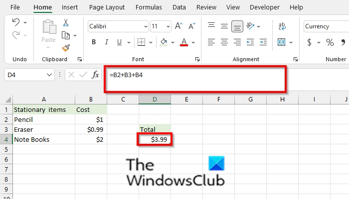
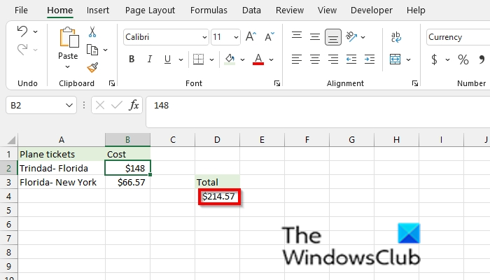
To fix this issue, remove the text and add the cost price.
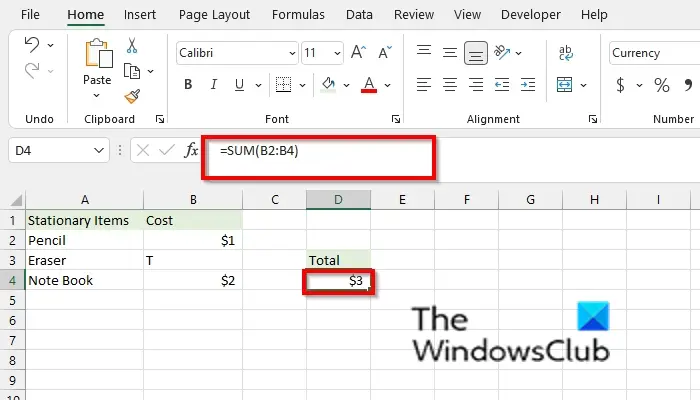
If you are using the Sum function, it will ignore the text and add the numbers of the two items in the spreadsheet.
2] The input of special characters
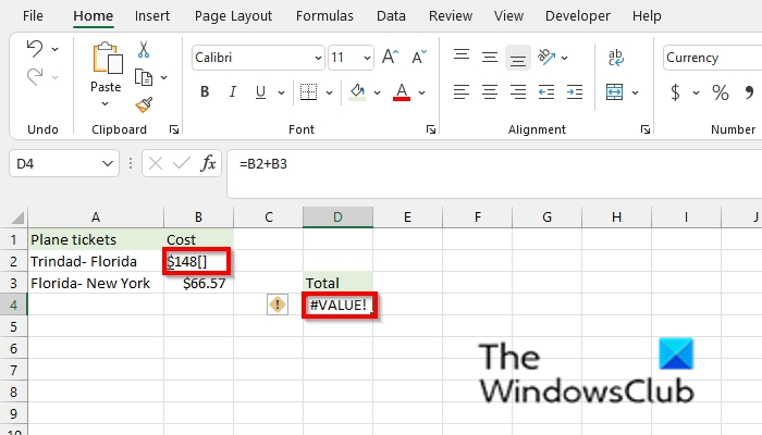
Inputting a special character into the data that you want to calculate can cause the #VALUE error.
To fix the issue, remove the space character.
3] The function argument is not the expected type
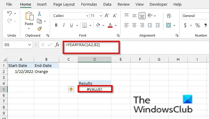
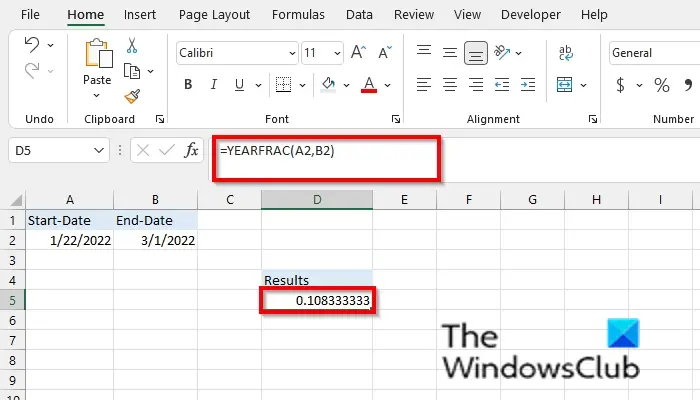
The error can occur when you input the wrong data that does not match with the function reference, for example, in the photo above the text, Orange does not go along with the YearFrac function. YearFrac is a function that returns a decimal value that represents the fractional years between two dates.
To fix this issue, enter the right data into the cell.
4] Dates stored as text
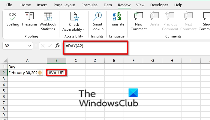
If dates are written in text, as seen in the photo above, you will see the Value error occur.
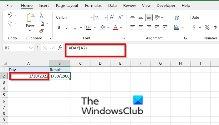
Enter the format correctly.
We hope this tutorial helps you understand how to fix the #Value error in Excel; if you have questions about the tutorial, let us know in the comments.
What is error in spreadsheet?
In Microsoft Excel, users will sometimes experience errors in Excel formulas. Errors usually occur when a reference becomes invalid (when there is an incorrect reference in your functions, or columns are rows are removed.)
How do you show errors in Excel?
If you have lots of data or a large table containing data on your spreadsheet and you want to find errors in it, follow the steps below.
- Click the Formulas tab.
- Click the Error Checking button in the Formula Auditing group and click Error Checking in the drop-down list.
- An Error Checking dialog box will appear.
- Click Next.
- Then, you will see the error in the spreadsheet.
Hope this helps.

Shantel has studied Data Operations, Records Management, and Computer Information Systems. She is quite proficient in using Office software. Her goal is to become a Database Administrator or a System Administrator.

#VALUE error in Excel is displayed when the variable provided in the formula is not a supported type or when the cell referred to in the formula is invalid. It is Excel’s way of telling the user that the right kind of argument is not provided.
There can be several reasons why Excel displays this error and you need to find the exact reason for the specific error to fix it!
- What is #VALUE error in Excel?
- How to fix #VALUE error in Excel?
- Conclusion
What is #VALUE error in Excel?
When you enter unexpected data in a formula, it might display a #VALUE! error. This Excel error can occur because of one of the following reasons:
- Text is used in Arithmetic Operations; or
- Cell contains hidden spaces; or
- Date stored as text
Let’s consider different examples to examine each of these causes and learn how to fix them!
Follow this detailed tutorial on #value Excel and download this Excel workbook to practice along understand better:
How to fix #VALUE error in Excel?
Example 1: Text is used in Arithmetic Operations
Here, we are trying to calculate the total sales amount by adding the sales achieved in both regions on different dates.

As you can see when cell D7 adds B7 and C7, it returns #VALUE! error. This is because cell B7 contains text instead of a number.
Let’s fix this!
Change the text nil to number 0.

You can also use the function SUM instead of using the addition operator (+). As formulas with operators will not calculate cells with text and instead display VALUE error.
If you use functions they will simply ignore text values and calculate everything else.

Example 2: Cell contains hidden spaces
Sometimes, VALUE error will be displayed when the cell contains hidden spaces. These spaces will look like the cell is blank but in fact, it contains a space instead.
In this example, you can see even though cell B7 looks like it is a blank, value is cell D7 is displaying an error. This is because cell B7 actually contains hidden space!

There can be numerous cells that may contain hidden spaces and it may be difficult to spot and remove them.
So, follow these steps below to find extra spaces and remove them!
STEP 1: Select the range that contains hidden spaces.

STEP 2: Press Ctrl + F to open the Find & Replace dialog box and select Replace tab.

STEP 3: Type in an extra space in Find what field and keep Replace field blank.

STEP 3: Press Replace All button. This is remove all the hidden spaces in the selected cells and leave them blank.

All the errors will now disappear!

Example 3: Date stored as text
In this example, we are trying to add duration to the start day of the project in order to get the project’s end date
Here, cells C7 and C11 are displaying #VALUE! error as Excel cannot recognize the value as a date. This is because date is separated using the decimal points as delimiters.

Let’s change the delimiter from decimal point (.) to hyphen (-)!
STEP 1: Select the cells containing dates.

STEP 2: Press Ctrl+H to open Find & Replace dialog box.

STEP 3: Type decimal point in Find What field and hyphen in Replace With field.

STEP 4: Press Replace All button.

This will replace decimal point with hyphen. Excel will now treat them as dates and make your formula work perfectly.

Conclusion
Value error in Excel occurs when the value provided in the formula is not the expected type. And, once you fix that value the error will disappear.
Click here to learn about the Top 20 Common Errors that you may encounter while working on Excel.
HELPFUL RESOURCE:
Make sure to download our FREE PDF on the 333 Excel keyboard Shortcuts here:

You can learn more about how to use Excel by viewing our FREE Excel webinar training on Formulas, Pivot Tables, Power Query, and Macros & VBA!
About The Author
John Michaloudis
John Michaloudis is the Founder & Chief Inspirational Officer of MyExcelOnline!