
Use data validation to restrict the type of data or the values that users enter into a cell, like a dropdown list.

Try it!
-
Select the cell(s) you want to create a rule for.
-
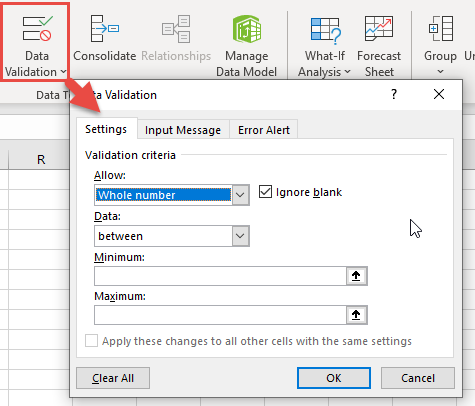
Select Data >Data Validation.

-
On the Settings tab, under Allow, select an option:
-
Whole Number — to restrict the cell to accept only whole numbers.
-
Decimal — to restrict the cell to accept only decimal numbers.
-
List — to pick data from the drop-down list.
-
Date — to restrict the cell to accept only date.
-
Time — to restrict the cell to accept only time.
-
Text Length — to restrict the length of the text.
-
Custom – for custom formula.
-
-
Under Data, select a condition.
-
Set the other required values based on what you chose for Allow and Data.
-
Select the Input Message tab and customize a message users will see when entering data.
-
Select the Show input message when cell is selected checkbox to display the message when the user selects or hovers over the selected cell(s).
-
Select the Error Alert tab to customize the error message and to choose a Style.
-
Select OK.
Now, if the user tries to enter a value that is not valid, an Error Alert appears with your customized message.
Download our examples
Download an example workbook with all data validation examples in this article
If you’re creating a sheet that requires users to enter data, you might want to restrict entry to a certain range of dates or numbers, or make sure that only positive whole numbers are entered. Excel can restrict data entry to certain cells by using data validation, prompt users to enter valid data when a cell is selected, and display an error message when a user enters invalid data.
Restrict data entry
-
Select the cells where you want to restrict data entry.
-
On the Data tab, click Data Validation > Data Validation.
Note: If the validation command is unavailable, the sheet might be protected or the workbook might be shared. You cannot change data validation settings if your workbook is shared or your sheet is protected. For more information about workbook protection, see Protect a workbook.
-
In the Allow box, select the type of data you want to allow, and fill in the limiting criteria and values.
Note: The boxes where you enter limiting values will be labeled based on the data and limiting criteria that you have chosen. For example, if you choose Date as your data type, you will be able to enter limiting values in minimum and maximum value boxes labeled Start Date and End Date.
Prompt users for valid entries
When users click in a cell that has data entry requirements, you can display a message that explains what data is valid.
-
Select the cells where you want to prompt users for valid data entries.
-
On the Data tab, click Data Validation > Data Validation.
Note: If the validation command is unavailable, the sheet might be protected or the workbook might be shared. You cannot change data validation settings if your workbook is shared or your sheet is protected. For more information about workbook protection, see Protect a workbook.
-
On the Input Message tab, select the Show input message when cell is selected check box.
-
In the Title box, type a title for your message.
-
In the Input message box, type the message that you want to display.
Display an error message when invalid data is entered
If you have data restrictions in place and a user enters invalid data into a cell, you can display a message that explains the error.
-
Select the cells where you want to display your error message.
-
On the Data tab, click Data Validation > Data Validation.
Note: If the validation command is unavailable, the sheet might be protected or the workbook might be shared. You cannot change data validation settings if your workbook is shared or your sheet is protected. For more information about workbook protection, see Protect a workbook.
-
On the Error Alert tab, in the Title box, type a title for your message.
-
In the Error message box, type the message that you want to display if invalid data is entered.
-
Do one of the following:
To
On the
Style
pop-up menu, selectRequire users to fix the error before proceeding
Stop
Warn users that data is invalid, and require them to select Yes or No to indicate if they want to continue
Warning
Warn users that data is invalid, but allow them to proceed after dismissing the warning message
Important
Add data validation to a cell or a range
Note: The first two steps in this section are for adding any type of data validation. Steps 3-7 are specifically for creating a drop-down list.
-
Select one or more cells to validate.
-
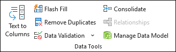
On the Data tab, in the Data Tools group, click Data Validation.
-
On the Settings tab, in the Allow box, select List.
-
In the Source box, type your list values, separated by commas. For example, type Low,Average,High.
-
Make sure that the In-cell dropdown check box is selected. Otherwise, you won’t be able to see the drop-down arrow next to the cell.
-
To specify how you want to handle blank (null) values, select or clear the Ignore blank check box.
-
Test the data validation to make sure that it is working correctly. Try entering both valid and invalid data in the cells to make sure that your settings are working as you intended and your messages are appearing when you expect.
Notes:
-
After you create your drop-down list, make sure it works the way you want. For example, you might want to check to see if the cell is wide enough to show all your entries.
-
Remove data validation — Select the cell or cells that contain the validation you want to delete, then go to Data > Data Validation and in the data validation dialog press the Clear All button, then click OK.
The following table lists other types of data validation and shows you ways to add it to your worksheets.
|
To do this: |
Follow these steps: |
|---|---|
|
Restrict data entry to whole numbers within limits. |
|
|
Restrict data entry to a decimal number within limits. |
|
|
Restrict data entry to a date within range of dates. |
|
|
Restrict data entry to a time within a time frame. |
|
|
Restrict data entry to text of a specified length. |
|
|
Calculate what is allowed based on the content of another cell. |
|
 in the Number group on the Home tab.
Notes:
-
The following examples use the Custom option where you write formulas to set your conditions. You don’t need to worry about whatever the Data box shows, as that’s disabled with the Custom option.
-
The screen shots in this article were taken in Excel 2016; but the functionality is the same in Excel for the web.
|
To make sure that |
Enter this formula |
|---|---|
|
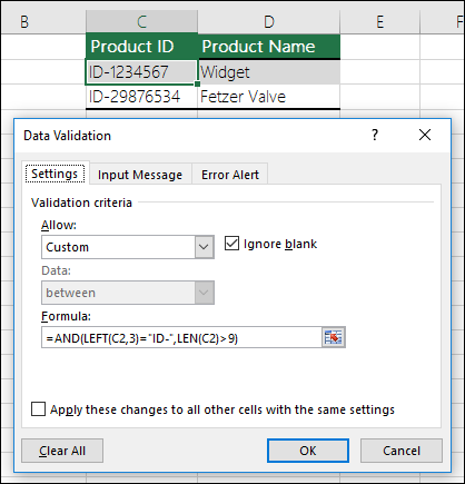
The cell that contains a product ID (C2) always begins with the standard prefix of «ID-» and is at least 10 (greater than 9) characters long. |
=AND(LEFT(C2,3)=»ID-«,LEN(C2)>9) |
|
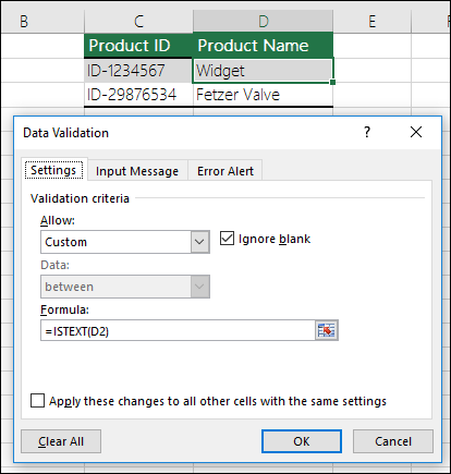
The cell that contains a product name (D2) only contains text. |
=ISTEXT(D2) |
|
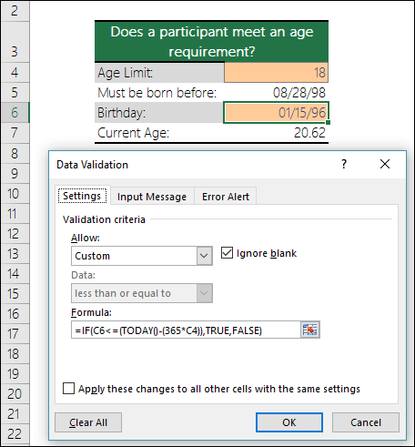
The cell that contains someone’s birthday (B6) has to be greater than the number of years set in cell B4. |
=IF(B6<=(TODAY()-(365*B4)),TRUE,FALSE) |
|
All the data in the cell range A2:A10 contains unique values. |
=COUNTIF($A$2:$A$10,A2)=1 Note: You must enter the data validation formula for cell A2 first, then copy A2 to A3:A10 so that the second argument to the COUNTIF will match the current cell. That is the A2)=1 portion will change to A3)=1, A4)=1 and so on. For more information |
|
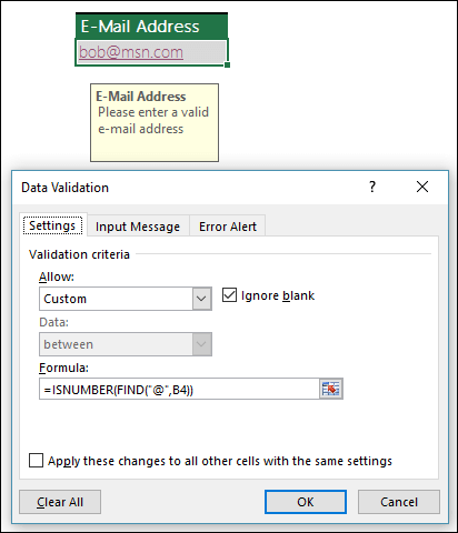
Ensure that an e-mail address entry in cell B4 contains the @ symbol. |
=ISNUMBER(FIND(«@»,B4)) |

Tip: If you’re a small business owner looking for more information on how to get Microsoft 365 set up, visit Small business help & learning.
Want more?

Create a drop-down list
Add or remove items from a drop-down list
More on data validation
See all How-To Articles
Data Validation is a tool in Excel that lets you restrict which entries are valid in a cell. Here are 10 rules and techniques to help you make the most out of Data Validation and its many features.
- Use Drop-Down Lists
- Data Validation Based on Another Cell
- ToolTips and Error Messages
- Options and Settings
- Date and Time Formats
- Set a Character Limit
- Validate Phone Numbers and Emails
- Custom Formulas
- Change or Remove Data Validation Rules
- Issues and Fixes
Use Drop-Down Lists
The most useful type of data validation is the drop-down list feature. For instructions on creating a drop-down list, see Create or Add a Drop-Down List in Excel and Google Sheets.
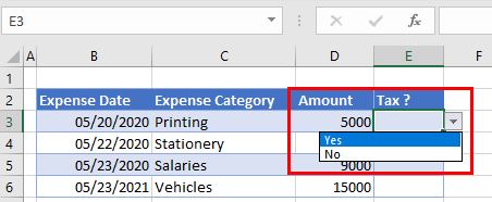
There are plenty of uses for drop-down lists and many ways to create them. For example, a simple yes/no drop-down list like the one below can be added as a quick and dependable indicator in a spreadsheet.
You can also use VBA to create a drop-down list in a cell. Enter this code in the VBA editor:
Sub DropDownListinVBA()
Range("A2").Validation.Add Type:=xlValidateList, AlertStyle:=xlValidAlertStop, _
Formula1:="Orange,Apple,Mango,Pear,Peach"
End Sub
Dynamic Drop-Down Lists
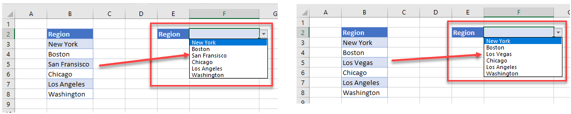
- When you create a drop-down list based on a range of cells using a data validation rule, if the data in that specific range changes, then the values in the drop-down list also change.
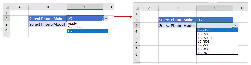
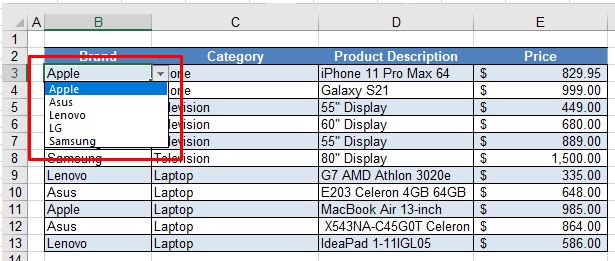
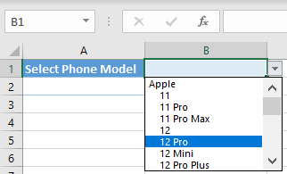
- Go a step further with a cascading drop-down list based on the value that is selected in a different list. In the example below, the user has selected LG as the Phone Make. The list of Phone Models then shows only the LG models. If the user were to select either Apple or Samsung, then the list would change to show the relevant models for those makes of phone.
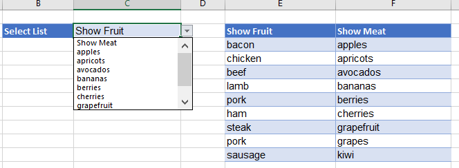
- An alternative method is to use an IF statement within the data validation feature to show a specific list that changes according to what the user selects. In the example below, if the user selects Show Fruit, then the fruit drop-down list is shown, whereas selecting Show Meat brings up the meat drop-down list.
Filter Data With a Drop-Down List
You can use Excel’s filter tool alongside a drop-down list for extended functionality.
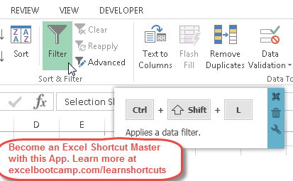
- Filters and drop-down lists are similar and even use the same keyboard shortcut (CTRL + SHIFT + L). In a data validation context, the shortcut activates a drop-down menu.
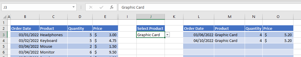
- A drop-down list can also be used as a filter in Excel. It enables you to extract rows of data that match the entry in the drop-down list and return these rows to a separate area of the worksheet.
Drop-Down List Formatting and Display Tools
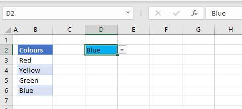
- If you want to create a drop-down list where the background color depends on the text selected, you can use Conditional Formatting to amend the background color when an item from the list is selected.
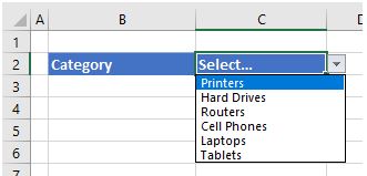
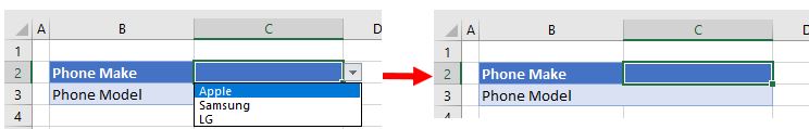
- When you create a drop-down list, the default value of the cell where you have placed the list is usually blank. It can be useful to pre-populate this cell with either a default value or a message to the user, such as Select…
- Once you’ve created a drop-down list, you can use the SORT and UNIQUE Functions to sort the drop-down list into alphabetical order.
- To make a drop-down list more readable, you can group a list of items by category (phone models in brand groups, for example).
AutoComplete Drop Down
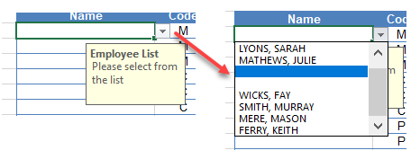
AutoComplete is a useful feature of Excel in that it can reduce the number of characters you need to type in each cell. The standard data validation drop-down functionality does not support AutoComplete. However, you can learn here how to approximate autocomplete with a drop-down list. Then, when you start typing the first letters of an entry in the drop-down list, the rest of the entry automatically shows up.
Drop Down Populates Another Cell
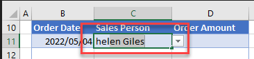
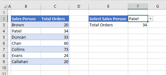
- Selecting an item from a drop down can populate a different cell in Excel and Google Sheets. For example, in the graphic below, Patel is selected from the list, and the cell below is then populated with the value 34. You can learn how to do this by clicking here.
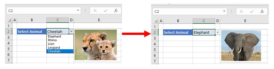
- Using a drop-down list, you can also insert a picture into another cell automatically.
Data Validation Based on Another Cell
When entering values in Excel, you can restrict the data that is entered into any range of cells based on text or a value held in another cell.
- When you create a drop-down list, you can write a custom input message that is seen on the screen when a cell is selected. This input message can also be referred to as a ToolTip.
- You can also customize the output (error alert) message that is returned to the user if invalid data is entered into a cell.
Options and Settings
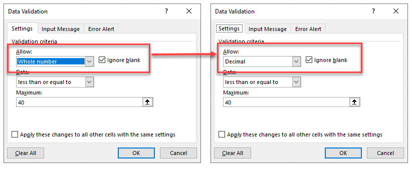
- There are seven different data types you can select from the Allow box of the Validation criteria: Whole number, Decimal, List, Date, Time, Text length, and Custom.
- The Ignore blank option is only available if you are actually editing a cell that has that option switched off.
- You can also choose, when editing a data validation rule, whether or not to apply the changes to other cells with the same settings.
Date and Time Formats
You can use Data Validation to restrict the format entered into a cell to ensure it is a date, and also to restrict the entry to be set between a start date and an end date.
Set a Character Limit
In Excel, the number of characters allowed in a single cell is 32767. However, you can set your own character limit for a text cell.
Validate Phone Numbers and Emails
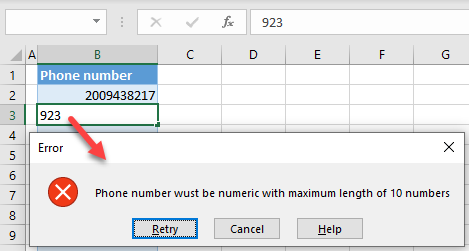
- You can use Data Validation to ensure that a phone number is entered correctly into Excel.
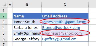
- You can also use Data Validation to ensure that an email address contains a @ sign and does not have any spaces or commas in it.
Custom Formulas
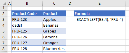
You can write a custom formula to make your own data validation rules. In the example below, the formula ensures that the data in a cell begins with certain text.
Custom Formula Examples
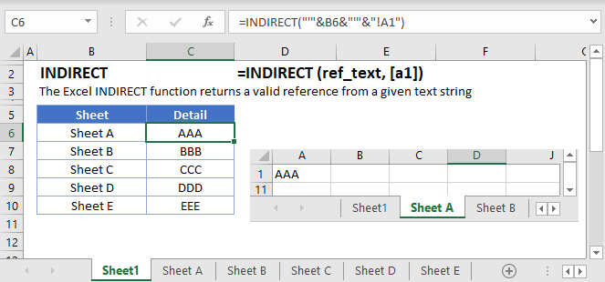
- You can use the INDIRECT Function in Excel in conjunction with a data validation drop-down list to create a cell reference from text.
- Use the ISNUMBER Function to check that the data inputted is in fact, a number. Data Validation has a built-in Whole number option, but you can generalize further with a custom formula.
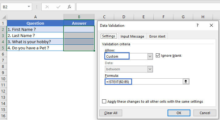
- Use a the ISTEXT Function to check for text. The example below allows only text values in the cells with data validation applied.
- You can use a data validation drop down with the COUNTIF Function to count cells that meet certain criteria and return a total.
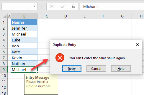
- COUNTIF is also useful for preventing users from entering duplicate values.
- A risk score matrix is a matrix that is used during risk assessment in order to calculate a risk value by inputting the likelihood and consequence of an event. You can use a data validation drop down in conjunction with the VLOOKUP and MATCH Functions to create a risk score matrix.
Change or Remove Data Validation Rules
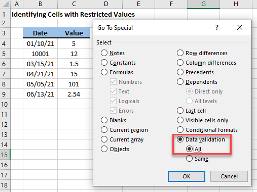
- If you have a data validation rule set in Excel, you can find any restricted values by selecting Data validation in the Go To Special dialog box.
- You can copy data validation rules from one set of cells to another set of cells by using the Paste Special command (CTRL + ALT + V).
- If you already have rules set up in a worksheet, you can amend the validation rules should your requirements change.
- You can amend the contents of a drop-down list by following the instructions in this tutorial.
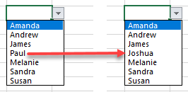
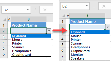
- You can easily update (change, extend, or have fewer items) a drop-down list by adding or deleting items from the list’s source range.
- If data validation on a range is no longer required, you can remove it.
- If you no longer require a drop-down list, you can easily remove the data validation settings by following the instructions in this tutorial.
Issues and Fixes
- If you have a value in Google Sheets that does not match the items in your drop-down list (an invalid item), you get a red triangle in the top left corner of the cell. To get rid of this triangle, you can follow the steps in this tutorial.
- There are a number of reasons why your data validation rule or drop-down list is not working correctly. You can troubleshoot these issues by referring to this tutorial.
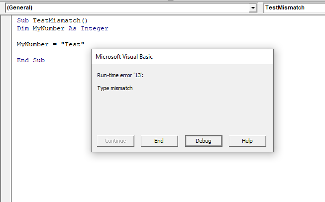
- A mismatch error can occur when you run VBA code. The error stops your code from running completely and flags the error by means of a message box. One of the ways you can prevent this from happening is to use Data Validation on the spreadsheet to prevent the user from causing worksheet errors in the first place. Only allow them to enter values that don’t cause worksheet errors.
Introduction
Data validation is a feature in Excel used to control what a user can enter into a cell. For example, you could use data validation to make sure a value is a number between 1 and 6, make sure a date occurs in the next 30 days, or make sure a text entry is less than 25 characters.
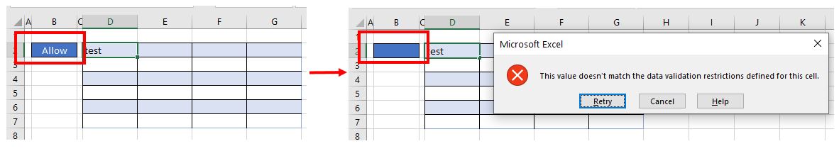
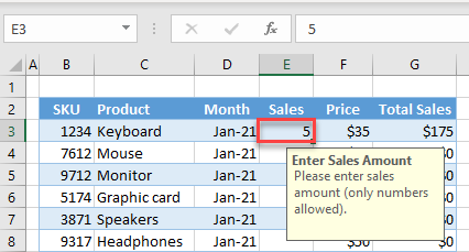
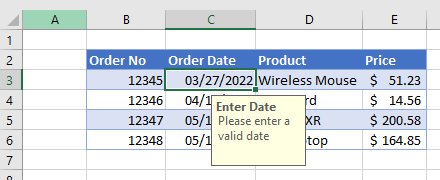
Data validation can simply display a message to a user telling them what is allowed as shown below:

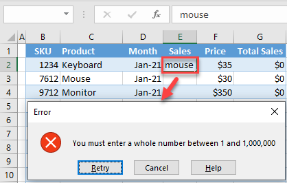
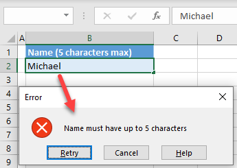
Data validation can also stop invalid user input. For example, if a product code fails validation, you can display a message like this:
")
In addition, data validation can be used to present the user with a predefined choice in a dropdown menu:

This can be a convenient way to give a user exactly the values that meet requirements.
Data validation controls
Data validation is implemented via rules defined in Excel’s user interface on the Data tab of the ribbon.

Important limitation
It is important to understand that data validation can be easily defeated. If a user copies data from a cell without validation to a cell with data validation, the validation is destroyed (or replaced). Data validation is a good way to let users know what is allowed or expected, but it is not a foolproof way to guarantee input.
Defining data validation rules
Data validation is defined in a window with 3 tabs: Settings, Input Message, and Error Alert:

The settings tab is where you enter validation criteria. There are a number of built-in validation rules with various options, or you can select Custom, and use your own formula to validate input as seen below:

The Input Message tab defines a message to display when a cell with validation rules is selected. This Input Message is completely optional. If no input message is set, no message appears when a user selects a cell with data validation applied. The input message has no effect on what the user can enter — it simply displays a message to let the user know what is allowed or expected.

The Error Alert Tab controls how validation is enforced. For example, when style is set to «Stop», invalid data triggers a window with a message, and the input is not allowed.

The user sees a message like this:

When style is set to Information or Warning, a different icon is displayed with a custom message, but the user can ignore the message and enter values that don’t pass validation. The table below summarizes behavior for each error alert option.
| Alert Style | Behavior |
|---|---|
| Stop | Stops users from entering invalid data in a cell. Users can retry, but must enter a value that passes data validation. The Stop alert window has two options: Retry and Cancel. |
| Warning | Warns users that data is invalid. The warning does nothing to stop invalid data. The Warning alert window has three options: Yes (to accept invalid data), No (to edit invalid data) and Cancel (to remove the invalid data). |
| Information | Informs users that data is invalid. This message does nothing to stop invalid data. The Information alert window has 2 options: OK to accept invalid data, and Cancel to remove it. |
Data validation options
When a data validation rule is created, there are eight options available to validate user input:
Any Value — no validation is performed. Note: if data validation was previously applied with a set Input Message, the message will still display when the cell is selected, even when Any Value is selected.
Whole Number — only whole numbers are allowed. Once the whole number option is selected, other options become available to further limit input. For example, you can require a whole number between 1 and 10.
Decimal — works like the whole number option, but allows decimal values. For example, with the Decimal option configured to allow values between 0 and 3, values like .5, 2.5, and 3.1 are all allowed.
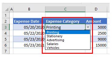
List — only values from a predefined list are allowed. The values are presented to the user as a dropdown menu control. Allowed values can be hardcoded directly into the Settings tab, or specified as a range on the worksheet.
Date — only dates are allowed. For example, you can require a date between January 1, 2018 and December 31 2021, or a date after June 1, 2018.
Time — only times are allowed. For example, you can require a time between 9:00 AM and 5:00 PM, or only allow times after 12:00 PM.
Text length — validates input based on number of characters or digits. For example, you could require code that contains 5 digits.
Custom — validates user input using a custom formula. In other words, you can write your own formula to validate input. Custom formulas greatly extend the options for data validation. For example, you could use a formula to ensure a value is uppercase, a value contains «xyz», or a date is a weekday in the next 45 days.
The settings tab also includes two checkboxes:
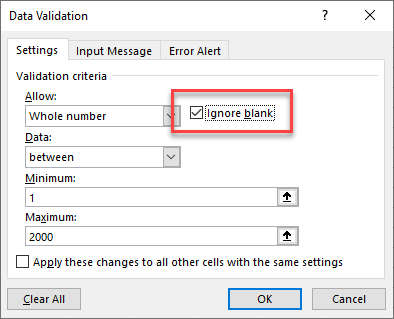
Ignore blank — tells Excel to not validate cells that contain no value. In practice, this setting seems to affect only the command «circle invalid data». When enabled, blank cells are not circled even if they fail validation.
Apply these changes to other cells with the same settings — this setting will update validation applied to other cells when it matches the (original) validation of the cell(s) being edited.
Note: You can also manually select all cells with data validation applied using Go To + Special, as explained below.
Simple drop down menu
You can provide a dropdown menu of options by hardcoding values into the settings box, or selecting a range on the worksheet. For example, to restrict entries to the actions «BUY», «HOLD», or «SELL» you can enter these values separated with commas as seen below:

When applied to a cell in the worksheet, the dropdown menu works like this:

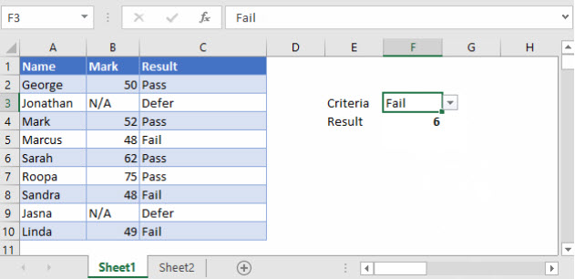
Another way to supply values to a dropdown menu is to use a worksheet reference. For example, with sizes (i.e. small, medium, etc.) in the range F3:F6, you can supply this range directly inside the data validation settings window:
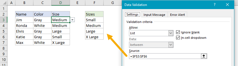
Note the range is entered as an absolute address to prevent it from changing as the data validation is applied to other cells.
Tip: Click the small arrow icon at the far right of the source field to make a selection directly on the worksheet so you don’t have to enter the range manually.
You can also use named ranges to specify values. For example, with the named range called «sizes» for F3:F7, you can enter the name directly in the window, starting with an equal sign:

Named ranges are automatically absolute, so they won’t change as the data validation is applied to different cells. If named ranges are new to you, this page has a good overview and a number of related tips.
Tip — if you use an Excel Table for dropdown values, Excel will expand or contract the table automatically when dropdown values are added or removed. In other words, Excel will automatically keep the dropdown in sync with values in the table as values are changed, added, or removed. If you’re new to Excel Tables, you can see a demo in this video on Table shortcuts.
Data validation with a custom formula
Data validation formulas must be logical formulas that return TRUE when input is valid and FALSE when input is invalid. For example, to allow any number as input in cell A1, you could use the ISNUMBER function in a formula like this:
=ISNUMBER(A1)
If a user enters a value like 10 in A1, ISNUMBER returns TRUE and data validation succeeds. If they enter a value like «apple» in A1, ISNUMBER returns FALSE and data validation fails.
To enable data validation with a formula, selected «Custom» in the settings tab, then enter a formula in the formula bar beginning with an equal sign (=) as usual.
Troubleshooting formulas
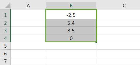
Excel ignores data validation formulas that return errors. If a formula isn’t working, and you can’t figure out why, set up dummy formulas to make sure the formula is performing as you expect. Dummy formulas are simply data validation formulas entered directly on the worksheet so that you can see what they return easily. The screen below shows an example:

Once you get the dummy formula working like you want, simply copy and paste it into the data validation formula area.
If this dummy formula idea is confusing to you, watch this video, which shows how to use dummy formulas to perfect conditional formatting formulas. The concept is exactly the same.
Data validation formula examples
The possibilities for data validation custom formulas are virtually unlimited. Here are a few examples to give you some inspiration:
To allow only 5 character values that begin with «z» you could use:
=AND(LEFT(A1)="z",LEN(A1)=5)
This formula returns TRUE only when a code is 5 digits long and starts with «z». The two circled values return FALSE with this formula.
To allow only a date within 30 days of today:
=AND(A1>TODAY(),A1<=(TODAY()+30))
To allow only unique values:
=COUNTIF(range,A1)<2
To allow only an email address
=ISNUMBER(FIND("@",A1)
Data validation to circle invalid entries
Once data validation is applied, you can ask Excel to circle previously entered invalid values. On the Data tab of the ribbon, click Data Validation and select «Circle Invalid Data»:

For example, the screen below shows values circled that fail validation with this custom formula:
=AND(LEFT(A1)="z",LEN(A1)=5)

Find cells with data validation
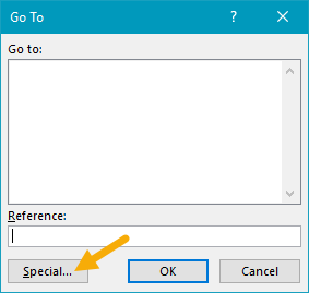
To find cells with data validation applied, you can use the Go To > Special dialog. Type the keyboard shortcut Control + G, then click the Special button. When the Dialog appears, select «Data Validation»:

Copy data validation from one cell to another
To copy validation from one cell to other cells. Copy the cell(s) normally that contain the data validation you want, then use Paste Special + Validation. Once the dialog appears, type «n» to select validation, or click validation with the mouse.

Note: you can use the keyboard shortcut Control + Alt + V to invoke Paste Special without the mouse.
Clear all data validation
To clear all data validation from a range of cells, make the selection, then click the Data Validation button on the Data tab of the ribbon. Then click the «Clear All» button:

To clear all data validation from a worksheet, select the entire worksheet, then, follow the same steps above.
The data validation in excel helps control the kind of input entered by a user in the worksheet. In other words, the input typed in a specific cell must comply with the criteria set for that cell. Data validation also allows providing instructions to the user about the input to be typed. The cell to which the data validation rule is applied is called a validated cell.
For example, the following data validation rules can be created in certain cells of Excel:
- A whole number between 1 (minimum) and 20 (maximum) is allowed.
- A date is allowed to be entered which is greater than September 15, 2000 (start date) or lesser than September 15, 2020 (end date).
- A text entry is allowed which matches any of the values (“yes,” “no,” and “cannot say”) of a drop-down list.
The pointers “a,” “b,” and “c” are the validating criteria defined for certain cells. If the input in these cells does not correspond to the respective pointer (a, b, or c), an error alert message is displayed by Excel.
Apart from setting the criteria, data validation in excel also allows to create a pre-defined range of inputs (drop-down list). In such cases, the user is asked to select the appropriate option (input) from this range. This ensures that all the data entries follow the same format.
Since the entries of all users are standardized, data validation brings about consistency and reduces errors. The “data validation” option is available in the “data tools” group of the Data tab of Excel.
Table of contents
- What is Data Validation in Excel?
- How to Use Data Validation in Excel?
- Example #1–“Data Validation” Window Explained
- Example #2–Decimal Number Validation
- Data Formats in Data validation
- The Different Validation Criteria
- The Different Error Alert Styles
- Purpose of Data Validation in Excel
- The Limitations of Data Validation in Excel
- Frequently Asked Questions
- Recommended Articles
- How to Use Data Validation in Excel?
How to Use Data Validation in Excel?
Let us consider some examples to understand the working of the data validation feature of Excel.
You can download this Data Validation Excel Template here – Data Validation Excel Template
Example #1–“Data Validation” Window Explained
The following image shows a list of numbers in column B. We want to perform the following tasks:
- Show how to create a data validation rule on the range B1:B4.
- Explain the tabs of the “data validation” window.
The steps explaining the creation of a data validation rule in Excel are listed as follows:
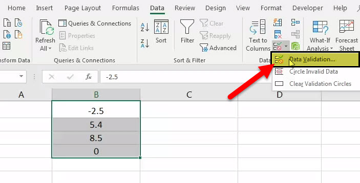
- Select the cells on which the data validation rule has to be created. So, select the range B1:B4.

- Click the data validation drop-down (in the “data tools” group) from the Data tab of Excel. The same is shown in the following image.

- Select “data validation” from the drop-down list.

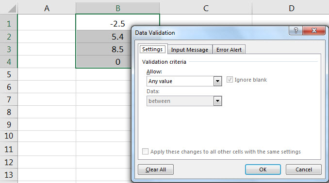
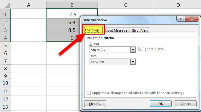
- The “data validation” window appears, as shown in the following image.

- The first tab is “settings,” which contains the validation criteria. The same is shown in the succeeding image.
From the drop-down list under “allow,” one can select the data format allowed to the users. The drop-down list under “data” is used for defining the criteria.
For instance, if the input should be entered as a whole number, select the same from the drop-down list under “allow.” Once “whole number” is selected, one can choose the minimum and the maximum range between which this number is allowed to be entered.
Likewise, the desired validation criteria can be defined for the user.
Note: Refer to the topics “The Different Data Formats” and “The Different Validation Criteria” of this article for more information on adding validation criteria.
- The checkbox “ignore blank” is selected by default. This selection tells Excel to ignore the blank values.
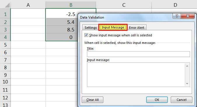
- The second tab is “input message,” as shown in the succeeding image. One can enter the “title” and the “input message,” which are displayed when a validated cell is selected.
Note: An “input message” tells the user about the kind of input allowed in a validated cell. However, it is optional to add an input message. But, if one does add an input message, ensure that the checkbox of “show input message when cell is selected” is checked.

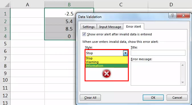
- The third tab is “error alert.” In this tab, one can enter the “title” and the “error message” that are displayed on typing invalid data in the validated cell.
From the “style” drop-down, one can select any of the three options, “stop,” “warning” or “information.” These are shown in the succeeding image.
Note 1: An “error message” is a customized message which tells the user that he/she has made an error while typing data in the validated cell. However, it is optional to add an error message. If an error message is added, ensure that the checkbox of “show error alert after invalid data is entered” is checked.
Note 2: In case an error message is not added, Excel displays the default error message, which states that restrictions have been defined for the validated cell.
Note 3: For more information on the error alert styles, refer to the topic “The Different Error Alert Styles” of this article.

- Once the entries in the three tabs, “settings,” “input message,” and “error alert” have been defined, click “Ok” in the “data validation” window.
The data validation excel rule is applied to the selected range B1:B4. Likewise, one can create a data validation rule by selecting either a single cell or a range of cells in Excel.
Note: For creating a data validation rule, it is mandatory to enter the validation criteria in the “settings” tab (step 5). However, it is optional to define the tabs “input message” (step 7) and “error alert” (step 8).

Example #2–Decimal Number Validation
Working on the data of example #1, we want to perform the following tasks:
- Create a data validation excel rule on cell B1. In this cell, a decimal number greater than or equal to zero is allowed to be entered.
- Define an input message which appears on selecting cell B1. The title should be “negative number detected” and the message should be “enter number greater than zero.”
The steps for performing the stated tasks are listed as follows:
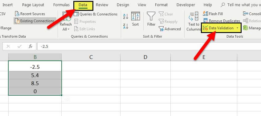
Step 1: Select cell B1 which contains -2.5. From the Data tab of Excel, click the “data validation” drop-down. Select “data validation.”
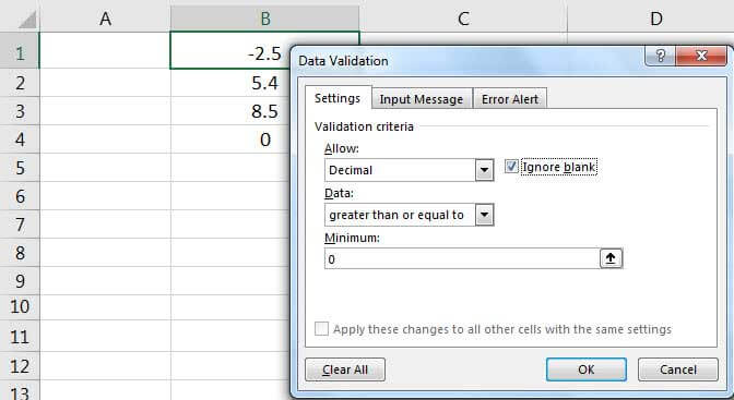
Step 2: The “data validation” window appears, as shown in the following image. In the “settings” tab, select “decimal” under the “allow” drop-down.
Under the “data” drop-down, select “greater than or equal to.” In the box under “minimum,” enter “0” (without the double quotation marks).
Step 3: In the “input message” tab, select the checkbox of “show input message when cell is selected.”
In the box under “title,” type “negative number detected” without the double quotation marks. In the box “input message,” type “enter number greater than zero.” This should also be written without the double quotation marks. Click “Ok.”
The data validation rule is created on cell B1. To cross-check it, select the validated cell B1. The defined input message appears, as shown in the following image.
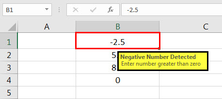
The number -2.5 was already there in cell B1 before the creation of the validation rule. This number is not deleted (from cell B1) even after creating a data validation rule.
However, in future, if a number is entered in cell B1, it must conform to the newly created rule. This implies that a decimal number greater than or equal to zero can be entered in cell B1. So, negative numbers are restricted in this cell. In case this rule is not complied with, Excel will display the default error alert.
Data Formats in Data validation
While entering data in a validated cell, there are certain formats that are allowed to the user. The rule creator (who is creating the data validation rule) can pick any of these formats based on which a validation rule can be created.
In the “settings” tab of the “data validation” window, the “allow” drop-down shows the following formats:
- Any value: This implies that no validation will be executed. In case a data validation rule is created and then “any value” is selected, the created validation rule is removed. However, the input message of the created validation rule can be viewed even after “any value” has been selected.
- Whole number: This requires that the user should enter a whole number in the validated cell.
- Decimal: This implies that the data format allowed in the validated cell is decimal numbers.
- List: This implies that the format allowed is a drop-down list. So, a drop-down list consisting of pre-defined values needs to be created. This drop-down list can be created in any of the following ways:
- Supply the values directly in the box under “source.”
- Provide the reference to the range (in the “source” box), which consists of the required values.
- Enter the name of the named range (in the “source” box), which begins with an “equal to” (=) sign.
- Date: This implies that the user can enter only a date in the validated cell.
- Time: This implies that a time value should be entered in the validated cell.
- Text Length: This helps fix the number of digits or text entered in a validated cell. For instance, the user can enter either numbers or text up to 5 digits or 5 characters respectively.
- Custom: This allows one to create a formula. This formula is used to validate (restrict) the input entered by the user. For instance, a formula can be entered to ensure that a text entry ends with certain characters, the text should be in uppercase or the entry must only be numeric, etc.
The Different Validation Criteria
Excel presents different criteria for validating data. The rule creator can select any of these criteria. Based on this selection, one can set the limits within which the input is allowed.
In the “settings” tab of the “data validation” dialog box, the drop-down under “data” shows the following validating criteria:
- Between: This implies that the input should be between the minimum and the maximum numbers specified.
- Not between: This implies that the input should not be between the minimum and the maximum numbers specified.
- Equal to: This implies that the input should be equal to the specified value. In other words, the input should be the same as the specified value.
- Not equal to: This implies that the input should not be equal to the specified value. In other words, the input should be different from the specified value.
- Greater than: This implies that the input should be greater than the minimum number specified.
- Less than: This implies that the input should be lesser than the maximum number specified.
- Greater than or equal to: This implies that the input should be greater than or equal to the minimum number specified.
- Less than or equal to: This implies that the input should be lesser than or equal to the maximum number specified.
The Different Error Alert Styles
There are different error alert styles in Excel. The rule creator can select any of these styles to notify the user that an error has been made while typing data in the validated cell.
In the “error alert” tab of the “data validation” window, the drop-down under “style” presents the following options:
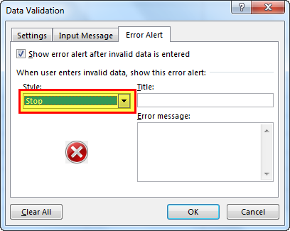
- Stop: This stops the users from entering invalid data in the validated cell. With the “stop” style, the error alert message presents the following main options to the user:
- Retry– Clicking “retry” allows typing a new input.
- Cancel–Clicking “cancel” deletes the invalid input.
The “stop” style is the default error alert style of Excel.
- Warning: This warns the users that an invalid input has been entered. However, it does not stop the user from entering incorrect data. With the “warning” style, the user is presented with the following main options:
- Yes–Clicking “yes” makes Excel accept the invalid input.
- No–Clicking “no” allows typing a new input.
- Cancel–Clicking “cancel” deletes the invalid input.
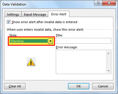
- Information: This informs the user that the input entered is invalid. Like the “warning” style, this also does not stop the user from entering incorrect data. With the “information” style, the user is presented with the following main options:
- Ok–Clicking “Ok” makes Excel accept the invalid input.
- Cancel–Clicking “cancel” deletes the invalid input.

By selecting a style, its respective icon appears in the error alert message displayed by Excel.
For instance, with the “stop” style, the cross within the red circle is shown (in the error alert message) as the user enters invalid data. Likewise, with the “warning” and “information” styles, the exclamation mark (within a yellow triangle) and the “i” sign (within a blue circle) show up respectively.
Note: Apart from the main options listed (in the preceding pointers 1, 2, and 3), Excel also displays the “help” option in all the error alert messages, irrespective of the style selected.
Purpose of Data Validation in Excel
The objectives of data validation in excel are listed as follows:
- To restrict the users from entering unwanted or incorrect data values in the worksheet
- To sort and study the data obtained with the help of defined criteria
- To suggest the valid data format to the users through customized input messages (displayed when a validated cell is selected)
Excel Data validation is particularly helpful in the following situations:
- When the number of users is large and there is a possibility of entering inputs in different formats
- When the allowed entries need to be defined with a drop-down list
- When an error alert (warning message) needs to be displayed on entering invalid data
The Limitations of Data Validation in Excel
The limitations of data validation in excel are listed as follows:
- Data validation in excel does not prevent a user from copying an incorrect input from a non-validated cell to a validated cell. It can stop one from typing an incorrect input but not from copying the same. Hence, the purpose of data validation can become pointless if a user copies and pastes an invalid input.
- Excel Data validation cannot fully protect a worksheet from invalid data entries. If a user copies an incorrect input from a non-validated cell and pastes it in a validated cell, the validation rule in the latter cell is eliminated. As a result, the validation rule is absent on the copied data.
Frequently Asked Questions
1. Define data validation in Excel.
Data validation restricts (limits) the type of input entered by a user in the worksheet. One can set the criteria for a specific cell and ensure that the input typed (in that cell) complies with it.
For instance, in cell A1, one is allowed to type only a decimal number between 1.5 and 9.5. This is a data validation rule applied to cell A1 of the worksheet.
2. How can a data validation rule be edited in Excel?
Let us say that rule X has been applied to cells A1 and D1. We want to change this to rule Y for both the mentioned cells.
The steps to edit a data validation rule are listed as follows:
a. Select any of the cells to which rule X has been applied.
b. Select “data validation” from the “data validation” drop-down (in the “data tools” group) of the Data tab.
c. In the “settings” tab of the “data validation” window, enter the new criteria as per rule Y.
d. Select the checkbox of “apply these changes to all other cells with the same settings.” This ensures that rule Y is applied to both the cells A1 and D1.
e. Click “Ok.”
The rule Y has been applied to both cells A1 and D1.
Note: The new data validation rule can be applied to all the validated cells only if they all had the same validation criteria initially. In this case, the initial validation criterion (rule X) was the same for both the validated cells (A1 and D1).
3. How can a data validation rule be removed in Excel?
The steps to remove (delete) a data validation rule are listed as follows:
a. Select the validated cell.
b. From the “data validation” drop-down (in the “data tools” group) of the Data tab, select “data validation.”
c. The “data validation” window opens. In the “settings” tab, click “clear all” appearing at the bottom left side.
d. Click “Ok.”
The validation rule will be cleared from the selected cell (selected in step a).
Note: To remove the same validation rule applied to multiple cells, select the checkbox of “apply these changes to all other cells with the same settings.” Thereafter, click “clear all” followed by “Ok.”
Recommended Articles
This has been a guide to data validation in Excel. Here we discuss how to create a data validation rule in Excel along with examples and downloadable Excel templates. You may also look at these useful functions in Excel–
- How to Insert a Checkbox in Excel?A checkbox in excel is a square box used for presenting options (or choices) to the user to choose from.read more
- PERCENTILE Excel FunctionThe PERCENTILE function is responsible for returning the nth percentile from a supplied set of values. read more
- Paste Special ShortcutsPaste special in Excel allows you to paste partial aspects of the data copied. There are several ways to paste special in Excel, including right-clicking on the target cell and selecting paste special, or using a shortcut such as CTRL+ALT+V or ALT+E+S.read more
- Data Table – ExamplesA data table in excel is a type of what-if analysis tool that allows you to compare variables and see how they impact the result and overall data. It can be found under the data tab in the what-if analysis section.read more
Having multiple users of a workbook is a perfect brew for a barrel of problems. Imagine anyone having access to editing anything. Your reports will quickly become subject to alteration, human errors, and someone’s quirks.
A complete shield against that would be protecting the sheet/workbook. This will lock the sheet/file from any alteration or you can choose the option of selective alteration where all the cells on the sheet are protected except chosen ones. Now if only you can control what type of data goes into the selectively open cells too?
Find that wish granted because in today’s Data Validation lineup, we’re going into the details of what Data Validation is, how to apply it, the limitations, the options and settings, some examples of Data Validation rules, and all the tidbits of finding, removing and copying Data Validation.
You have got to be wondering what the essence of Data Validation is so…
Let’s get validating!

What is Data Validation?
Data Validation in Excel limits the type of data users can enter into a cell. E.g., if you are entering game scores with a score range of 1 to 5, you can use Data Validation to control the scores that go in the target cells to be between 1 to 5.
While that is the prime role of Data Validation, its prime use is creating a drop-down menu for a cell.
The options in Excel provide a list of rules to choose from. These rules determine the type of data that can be entered on selected cells on the worksheet. It is here that you will find the option of adding a drop-down list.
Using these rules, you can control the data type in the cell to be only numbers, dates, time, and characters of a given length, selected from a drop-down list (list also created using Data Validation), or you can define the criteria through a custom formula. An Input Message can be displayed with a cell with or without a validation rule added.
When Data Validation is applied to a selection of cells and invalid data is entered by the user, an error alert will be displayed:

This is the default alert and through Data Validation, you can create a custom alert. Another feature of Data Validation is adding an Input Message to a cell that is quite identical to a comment in Excel.
That is what Excel’s Data Validation is in a nutshell. We’re sure you’re ready to jump to the how-to and we have it coming for you. We’ll begin with a simple case of adding Data Validation.
How to Add Data Validation?
Where will you find the Data Validation button? Hint: The Data tab. Everything you need from Data Validation can be found in the Data Validation icon in the Data Tools group. Now let’s see how to add Data Validation on the worksheet.
As a small example, let’s assume we are entering a passcode in a cell and you want it to pose an alert when an incorrect key is punched in. Use the steps ahead to add Data Validation to a cell to restrict the type of data that gets entered into the cell:
- Select the cell(s) you want to add Data Validation
- Go to the Data tab and click on the Data Validation icon in the Data Tools

- You will see a small Data Validation dialog box where all the main Data Validation business will take place. Currently, you can see that the validation criteria allow any value, without any restriction:

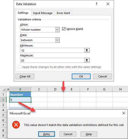
- We’re about to change that. In our example case, we want to ensure that all passcodes are 5-digit pins between 10000 to 99999. The Whole number rule will do for this.
- Make the following changes to the Data Validation settings:
- Click on the arrow in the Allow field and choose Whole number.
- In the Data drop-down list, select between.
- In the Minimum and Maximum fields, enter the smallest and largest number of the range you want to allow in the selected cell (i.e. 10000 and 99999 for us).

- When done, select the OK
The Data Validation dialog box will close. You will not see any overt changes since Data Validation is related to entering data. So go ahead and try to enter some invalid data in the cell e.g. we can try entering a 4-digit number. We will get an error alert.

The Retry button gives another attempt at entering the valid data type. The Cancel button wipes out the data we have entered and the Help button redirects us to the Microsoft Support webpage. So yes, you really have no way around this other than entering the relevant type of data.
Overriding Data Validation
Right now, Data Validation might be looking all types of invincible but it has a couple of chinks in its armor. The first is that if Data Validation is applied to occupied cells, the values will stay as they are; there will be no rectification and no notification or indication that the data is invalid.
Secondly, if invalid data is value-pasted to a cell containing a Data Validation rule, while the rule will still stand, the invalid data won’t be restricted from being pasted and there will again be no rectification or indication of invalid data.
This shows us that Data Validation is only a data-entry control and will only work for data that is being entered; not data that already exists or is being pasted.
Now that you’re getting a basic idea of what Data Validation does, we’ll explore the Data Validation dialog box before we go into the scope of Data Validation with some examples.
Excel Data Validation Options & Settings
You just saw how to access the Data Validation settings from the Data tab. Let’s go through the rules and options in the settings to understand what types of data entry Data Validation can control.
Settings
Firstly, the face of the Data Validation options; the Settings tab. To set validation criteria or rules, you begin with choosing a rule from the Allow menu. If you do not find a suitable preset criterion, you can use the Custom option. Here you will need a formula to define the Data Validation criteria. We’ll briefly go over the preset rules.

Any value
This is the default setting when no Data Validation is applied. Any value can be entered in the cells without any restriction. You can still add an Input Message to the cell(s) but for an error alert to show, there needs to be a rule in place.
Whole number
Allow only whole numbers to be entered in cells. You can further set the limit value(s) that will go into these cells once Data Validation is applied.

Additional fields become accessible with the rules. E.g. when you select the Whole number criteria, from the Data field you can choose if the number should fall between a provided range or should be equal to or greater/less than a certain value.
Decimal
This is the decimal variant of the Whole number rule since the latter doesn’t allow decimal. The options are the same with Decimal as they are with Whole number; only that the data entered will allow decimal and whole numbers that meet the specified range of values.
List
Create a drop-down list for a cell with this rule. The content of the list can be entered into the provided field in the Data Validation dialog box or can be referred to from the worksheet.

Unchecking the In-cell dropdown box will remove the drop-down menu which kind of kills the whole mojo of this rule but what will happen is that only the specified values can then be entered in the cell. The values manually entered using this rule will be case-sensitive.
Date
Restrict the data in the cells to be only entered as dates with the Date criterion. Set a start and/or end date to further limit the dates that will go on the worksheet.
Time
The Time rule will only allow time values in the cells. Entries can additionally be controlled by specifying the start and/or end time.
Text length
Text length limits the number of characters (whether numbers, letters, or symbols) that go into the cells.
Custom
Add a custom formula to expand the scope of Data Validation when you can’t find a match for your requirement in the predefined rules.
Checkbox – Ignore blank
Throughout the Data Validation rules, you may have noticed an Ignore blank checkbox. The role of this box is to ignore the blank cells from being treated as cells with invalid data since blank cells will not match most Data Validation criteria. Leave this box checked if you don’t want blank cells to be circled when circling invalid data (found out more about this feature later).
Checkbox – Apply these changes to all the other cells with the same settings
Let’s say you’ve selected a cell with Data Validation and open the Data Validation dialog box. When you mark this checkbox, all other cells on the worksheet that have the same validation criteria applied to them will be selected in the background.
This is useful if you don’t remember all the cells that you have applied a Data Validation rule to and want to select all the cells with that rule.
Button – Clear All
Clears Data Validation (comprising the validation rule and Input Message) from the selected cell, restoring the validation criterion to Any value.
Input Message
Onto the next tab in the Data Validation dialog box. This is the Input Message tab where you will learn about the settings regarding displaying an Input Message with a cell. The message will be displayed when the cell is selected and looks like an Excel cell comment.
This is an optional feature and merely a display item. Use an Input Message to notify a user about the contents of the cell, or the data type to be entered.
Let’s pick the example we were working on previously and see how we can add an Input Message to a cell.
- Select the cell(s) that you want displayed with the Input Message.
- Open the Data Validation dialog box from the Data tab > Data Tools group > Data Validation Then go to the Input Message tab.
- Enter the title (optional) to display as the Input Message header as we have added “Passcode”.
- Then add the Input Message in the given field.

- Click on the OK command to apply the settings.
Now, whenever that cell is selected, you will see the related Input Message in a pale yellow box.

You will not see the Input Message if the relevant cell is not selected. Uncheck the Show input message when cell is selected box to stop the message from appearing.
This will not affect the Data Validation rule and you can enable the message any time again. However, you can also clear the title and message from the Input Message tab if there will be no use for it later.
The Clear All button will reset the settings of the entire Data Validation dialog box, Settings tab included.
Error Alert
This tab deals with the error alert that will be displayed when invalid data is entered in the cells with Data Validation. Excel has three styles of error alerts to choose from with each style having different commands and control. Let’s run you through each of them so you know which error alert you would want to deploy.
The standard title of the alert is “Microsoft Excel” and the error message is «This value doesn’t match the data validation restrictions defined for this cell.» if nothing is specified otherwise.
Stop
The Stop alert is the default error alert displayed when you set a Data Validation rule. It appears with a cross icon. The title and error message can be added by the user which will overwrite the standard alert. The settings are the same for all error alerts.

The Stop alert restricts entering invalid data; with the Retry button, you will have to try entering the data again, the Cancel button will clear the entered data and the Help button will guide you to the support center.
Hence, with this alert style, there is no getting around «entering» invalid data. Why have we emphasized entering? There are ways around getting invalid data on the worksheet despite setting Data Validation and we’ll come to that later.

Use the Style list in the dialog box to switch to another alert style.
Warning
The Warning error alert, shown with an exclamation point icon is a softer alert that gives the user the option of retrying the entry (by using the No button) but also gives the space of continuing with the invalid entry (by using the Yes button).

Edit the title and message in the Data Validation dialog box if preferred.
Information
An even softer error alert form, the Information alert only lays out information (the default error message unless changed by the user) regarding the input data. Invalid data will still be accepted after clicking on the OK button. This alert is actually just like a reminder with hardly any restricting quality.

Other than the alert styles, in the Data Validation dialog box, there’s a Show error alert after invalid data is entered checkbox and if you unmark it, even with the Data Validation rule set, no validation will be performed.
The use of this checkbox makes sense to temporarily disable the validation so the rule and error style is still saved to be enabled later. Unmarking the checkbox is also of use when you want to give the user the option to choose from a Data Validation list and also of adding a new value.
Data Validation Examples
What we have covered majorly until now is how to add Data Validation, what the options and settings entail, and different types of error alerts. Now we’ll proceed to different examples where we can apply different Data Validation rules so you know how to use Data Validation for your worksheets.
Heading back to the Settings tab in the Data Validation dialog box, here goes the first rule.
Whole number
The first couple of steps of applying Data Validation is to select the target cells and to open the Data Validation dialog box to set the criteria. To open the dialog box, go to the Data tab > Data Tools group > Data Validation icon.
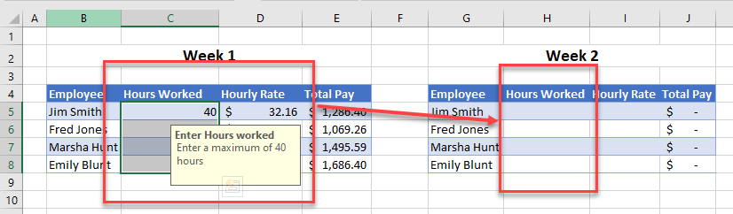
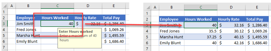
We’re working on the Whole number Data Validation criterion. In the case example below, we are filling out students’ marks in an exam. We have the Data criterion set to between to define what numbers the marks should be between.
The limits that we have set for the lowest marks is 0 and the highest has been set to 50 marks by entering F3 as an absolute reference so it remains fixed for the rest of the selection. Instead of entering 50 directly as the upper limit, we have referred a cell so that we can enter different total marks for tests and exams that Data Validation will automatically take into account.

Now click OK and try entering a number beyond the range of the specified limits. See what happens.

You will get an error alert and you will know that you have entered invalid data. Try re-entering the value in compliance with the Data Validation criteria.
The Decimal rule works in the same way; only that it allows decimal whereas the Whole number rule doesn’t. If you’re dealing with decimals and integers, you can apply the Decimal rule as it also allows integers in the specified range to be entered.
List
Creating a small and simple list would require nothing more than punching in the items of the intended list, delimited by commas, as the source:

But see this?

This comes readymade for no one but it can be achieved in some surprisingly simple steps. This is a drop-down menu created for every cell. For data entry, this is a dream and is made using the List rule in Data Validation.
But before we get to the List rule, we need to lay out a couple of things in advance. Create a list of the items you want in the drop-down menu, name that range, then create a Data Validation list with the Named Range.
The list for the Named Range can be on the same worksheet as the target validation data or a different sheet. If you prefer the list hidden, you can keep it on the same sheet in a white font. Now you can check out the steps to create in-cell drop-down menus with Data Validation using a Named Range from a separate sheet.
- Form a list of the items you want in the drop-down menu on a separate worksheet.

- Select the items of the list excluding the header.
- Click on the Name box in the corner and type a name for this list.

- After typing the name for the range (our Named Range is Services), hit the Enter

- The Named Range is ready.

- Now go back to the sheet where you’re entering the data. Select the cells that you want to add drop-down lists to.
- From the Data tab, select the Data Validation icon in the Data tools group.
- Choose List from the Allow
- Click on the Source field and press the F3

- A Paste Name box will be launched. Select the relevant Named Range, then press the OK

- The Named Range will appear in the Source field.
- Select the OK command on the Data Validation dialog box too.

The dialog box will close and the in-cell drop-down lists will be added to the selected cells. The arrow to access the drop-down list for a cell will appear when the cell is selected. Now the drop-down lists can be used to start data entry!
If an entry is punched in that doesn’t completely match one of the items of the list, it will be blocked by Data Validation.

Other than looking nifty, using in-cell drop-downs keeps the data entries consistent too.
Dynamic List
With a dynamic list, if you add an item to it, it will automatically be updated in the cell drop-down lists. The way to do that is to create an Excel Table out of the list (with header) along with making a Named Range out of it (without header).
Carrying on with the method we have shown you earlier, we can also extend the Named Range and the cell drop-downs will be updated as per the Named Range.
Let’s assume we are adding just one more service to the list. Add the item in the list that is on the separate sheet. Then select the original Named Range (Services in our case) without the new addition.

Open the Name Manager (Ctrl + F3 keys) and extend the range from B3:B9 to B3:B10. This will include the new item in the range.

Now when you check the in-cell drop-downs on the original sheet, it will include the new item!

The other method is to create a Table before naming the range. Select the list with the header and create a Table from the Home tab > Styles group > Format as Table icon, selecting a table style from the menu.

Once the same data is the items of a Table and Named Range, additions will automatically be incorporated in the cell drop-down lists. This works because an Excel Table is dynamic in nature and automatically includes additions.

The Table will also update the Named Range which will in turn update the in-cell drop-down menus.

Date
Use the Date rule to apply a Data Validation layer to dates in Excel. Not only will this ensure that the input data are dates but also that the dates are within the specified range.
For the example case, we have an extract of some sales data and are filling out the order and delivery dates of the products for the month of September. Begin by selecting the cells, opening the Data Validation dialog box, and selecting the Date criterion from the Allow section.
Now select between from the Data section to add the start and end dates. To keep the dates entered on the worksheet limited to September, the start date will be the 1st of September and the end date will be the 30th of September.
The dates can be fed directly in the dialog box or from the worksheet. To add them in the dialog box, use an Excel date format e.g. 9/1/2022.
Make sure to secure the dates as absolute references if added from the sheet and hit the OK button when done.

Any date added in the cells with Data Validation that is out of the range of the start and end dates will trigger the error alert.

Time
With the Time rule applied, no other input value will be accepted other than a time entry. Using a small example, we’ll show you the format to use in Data Validation for limiting the cells to contain a time value.
Setting up a meeting schedule for office hours would require the office timings as the start and end time. The format to use in the dialog box is 8:00:00 AM.
Tip: On the worksheet, change the format of a free cell to a Time format, enter the time and refer this cell in the Data Validation dialog box or copy the value and paste it in the dialog box.

Apply the rule and you won’t be able to enter values other than time within the mentioned time range set through Data Validation – confirms error alert.

Text length
We’ll now take an example where we are to limit the text length of a cell. You will be able to enter any type of character in text as long as the number of characters abides by the set text length.
As an example, we’ll confine the text length of our data column to equal 10 characters so that the phone numbers fed therein have a lesser chance of being subject to human error.
In the Data Validation dialog box, select the Text length rule. Choose the equal to option in the Data drop-down list and set the phone number digit length e.g., to 10.

Activate these settings by clicking OK. Data Validation will make sure that the entered phone numbers aren’t a single digit above or below 10.

Custom
This rule calls for a custom formula and the aim is to make it go beyond the functions of the preexisting rules in Data Validation and increase its scope. When it comes to custom formulas, there is so much that becomes open to us and that is why that calls for a whole section on its own.
Without further ado, we’ll start with Data Validation with custom formulas.
Formula-based Validation Rules
Earlier, we have been directly adding values or referring values from the worksheet to set the validation criteria which limits the use of Data Validation to the preset rules.
In this section, we are going to talk about using formulas in the preset and custom rules and throwing Excel functions into the works which will greatly expand Data Validation controls.
Dynamically limiting dates to 7 days before the current date, only entering weekdays, entering products of a specific code. This is definitely your regular Data Validation so learn how to do all of this below.
Tip: Using formulas in dialog boxes can be a little tricky because if it fails, it would be hard to pinpoint and tweak what part of the formula isn’t working. Use the formula on the worksheet first to see how it performs and then paste it in the dialog box.
7 Days Before & After TODAY
Let’s take today’s date as the 24th of September 2022. We’re filling out our worksheet containing the order and delivery dates of products that is forwarded daily to the dispatch department. The timeline is 15 days i.e. 7 days before and after the current date inclusive.
That makes our start and end date 17/9 and 1/10 respectively. And we can very well enter these dates directly but that will make a static limitation of the date range.
To keep the Data Validation dynamic, we’ll incorporate the TODAY function. The TODAY function returns the current date in the d/m/yyyy format. In the Data Validation dialog box, select Date and between as the first two criteria and enter the other two as:
Start date:
=TODAY()-7
End date:
=TODAY()+7
The start date is set to be 7 days before the current date and the end date is 7 days after. This keeps our range at 15 days.

For the current date, you will not be able to enter a day after 01-09-2022 and the next day the limit will become 02-09-2022 automatically.

Only Weekdays
Now let’s suppose we’re closed for the weekends; we will need to make sure that the delivery dates are only assigned to weekdays. Data Validation on its own wouldn’t know how to restrict date entries to just the weekdays but it can take the help of a formula and that’s where the WEEKDAY function comes in.
The WEEKDAY function, when fed a date, returns a number from 1 to 7 indicating the day of the week the date falls on.
Access the Data Validation dialog box from the Data tab and choose the Custom criteria. The only other requirement now will be a formula so enter this one in the given field:
=WEEKDAY(D3,2)<6
First off, the second argument of the WEEKDAY function, that is “2” in our example case, is the number for the type of week (Monday to Sunday). To pick a different week type, start punching the function on the worksheet and select the type from there.
In the formula mentioned above, the WEEKDAY function checks what day the date in D3 falls on (Tuesday in this case) and returns the number of Tuesday as per the selected week type. According to week type 2, Tuesday is the second day of the week so the outcome of the WEEKDAY function is 2.
In the other part of the formula, we have <6. With this bit, 6 being the number for Saturday, we are ensuring that the result of the WEEKDAY function is lesser than 6 and hence, earlier than Saturday. Since 2 is lesser than 6, the first date i.e. 20/9/2022 is good to go.

Try entering a weekend date; that’s foolproof Data Validation there:

Applying the same formula on the sheet confirms that the corresponding numbers of all the days are less than 6:

Beginning with Specific Characters
Data Validation can limit the entries beginning with specific characters. To track the entries, we’ll use the COUNTIF function that counts the number of cells in a range that fulfills the defined condition.
The product codes we are using in our case example are made up of product category initials (e.g. HL is for Home & Lifestyle) and then a 4-digit number code.
Use the following formula to only list the products with HL as the starting code:
=COUNTIF(B3,"HL-*")
Don’t worry about setting a different Data Validation rule separately if you’re aiming for two codes instead of one. Just add a plus sign + and repeat the formula with the other code:
=COUNTIF(B3,"HL-*")+COUNTIF(B3,"EA-*")
The COUNTIF function checks B3 for the code HL- in the beginning. The asterisk is added as a wildcard character that will take place of any number of characters in the formula since the product code will obviously have a different mix of numbers.

If the entry meets the condition of beginning with the code HL or EA, it will be accepted by Data Validation while the others will be blocked:

For grouping purposes, you’ll find sorting and filtering easier but for blocking other entries, Data Validation is the go-to. How would things change if, instead of the beginning, the characters were in the middle of the product code? Read on.
String Containing Specific Characters
By now, you have probably realized that we can get Data Validation to do so much more than the basics that it only becomes a matter of using the right formula.
If your characters of interest are anywhere in the string, beginning, mid or end, they can still come under the band of Data Validation using the FIND or SEARCH function.
The FIND function returns the position of the baby text string from the parent text string. You can use either of the two functions; the FIND function is case-sensitive while the SEARCH function is not. Use this formula with the Custom criteria in the Data Validation dialog box:
=FIND("HL",B3)
Just the FIND function on its own will restrict product codes without HL from being entered:

The formula didn’t find HL in the last code and so it cannot be entered:

You can apply this limitation regarding any character or number of characters. E.g. to allow only email IDs as the input, we can use the following formula:
=FIND("@",B3)
Assuming B3 is the first cell of the selection of the range where we are applying Data Validation.
No Duplicates
Here’s one more flex of Data Validation for the day; blocking duplicate entries. Making the COUNTIF function part of a custom formula, we can restrict repeated entries in the cells that Data Validation has been applied to.
Let’s take this example. While noting down entries for an interschool creative writing competition, we realized we could be making the same entry twice and we also realized that it would be a good idea to prevent that from happening in the first place.
Look at this formula and enter it in the formula field using the Custom rule in the Data Validation dialog box:
=COUNTIF($B$3:$B$17,B3)<2
The range that we want to keep free of duplicates is B3:B17. The condition is that the occurrence of B3 in the mentioned range should be less than 2 (you could also write =1). This way, any entry cannot be made twice as each input will be checked against the rest of the range.

An attempt at re-entering the same student failed!

Here’s some food for thought. The Goblet of Fire could have been secretly wired to Excel. Think about it.
Find Invalid Data on the Sheet
When you apply Data Validation to a dataset or paste values on Data Validation cells, you will not be notified of invalid data and it may seem that everything is spot on.
Indication: you will have to find the invalid data on the sheet. Good thing that’s not a very technically far-out problem. By invalid data, we are referring to the value in the cell not meeting the cell’s Data Validation criteria.
There’s an option in the Data Validation menu to circle all the invalid data on the sheet with a red border. We like to call that Excel’s teacher syndrome.
To find all the invalid data as per the Data Validation rule governing those cells, head to the Data tab’s Data Validation icon and click it and select the Circle Invalid Data option.

And that’s it! All the invalid data of all Data Validation rules on the sheet will be circled in red:

And when you want the teacher gone and want to take down all the red circles, use the Clear Validation Circles option or save the file to erase the highlighted invalid data.

If you find that the circling isn’t working properly, use Find & Select to ensure if Data Validation is applied to those cells or not because obviously; the data will be invalid only if Data Validation has been applied in the first place. Speaking of Find & Select, do you know how to use this feature for Data Validation?
How to Find Cells with Data Validation
You may have a good few Data Validation rules spread across your spreadsheet and you’re not about to manually check every other cluster of datasets for validation. Here’s an easy way to find out which cells are using Data Validation and it is with the Find & Select feature. Find & Select will select all the cells with Data Validation no matter how many rules and how dispersed they are.
To find all cells on the worksheet with Data Validation applied, on the Home tab, click on the Find & Select icon in the Editing group. From the menu, select Data Validation.

In our example case, we have applied one Data Validation rule on C3:C12 and another on F3. Both lots have been selected, confirming their Data Validation status.

Note: How does this method differ from the Apply these changes to all the other cells with the same settings checkbox? If you want to find the cells covered by all the Data Validation rules in a sheet, go ahead with Find & Select. To find the cells covered by one particular rule, go ahead with the checkbox.
How to Edit Data Validation Rules
Editing one Data Validation cell is easy from the settings but how do we edit all the cells that carry the same rule? While editing, there’s one small bit you need to take care of and it’s the Apply these changes to all the other cells with the same settings box.
You can edit cells of one rule at a time whether a single cell, a range of cells, or all the cells of a single rule. To edit all the cells belonging to a rule select any cell containing that rule and open the Data Validation dialog box using the Data Validation icon.

Edit the rule according to your requirement; we are changing the text length from 10 to 11 digits. Next, mark the Apply these changes to all the other cells with the same settings checkbox. As soon as you do, all the cells with the original rule will be selected in the background.

Apply the changes and check if you can get away with entering invalid data.

How to Remove Data Validation Rules
Removing Data Validation requires using the Clear All button in the Data Validation dialog box and how much Data Validation you want to remove will depend on the selection of cells.
Remove Data Validation from a single cell by selecting that cell and accessing the Data Validation dialog box. In the Settings tab, click the Clear All button in the bottom-left corner. This will clear the selected cell of the Data Validation rule and Input Message and will reset the Error Alert settings.

The OK command will seal the clearing of settings and you can see below that we are not bound to enter an 11-digit number now:

Remove Data Validation from all cells with the same rule
If there’s only one rule you want to dispose of, select any cell of that rule, open the Data Validation dialog box, select the Apply these changes to all the other cells with the same settings checkbox, click on the Clear All button, and then on the OK button.
Remove Data Validation from all cells on the sheet
Press Ctrl + A on the worksheet to select all the cells. Head to the Data Validation dialog box to use the Clear All button to remove all the Data Validation rules on the sheet.
Then hit the OK button.
How to Copy Data Validation to Other Cells
A plain copy & paste of a cell with Data Validation will paste the Data Validation rule and the value of the cell. To leave out the value and paste the rule, you can use the Validation option in Paste Special. If you don’t know how to use Paste Special, here’s what you need to do to copy Data Validation to other cells:
- To copy a particular Data Validation rule, select any cell with that rule and press the Ctrl + C keys to copy it.
- Now select the cell or the range where you want to paste the rule. Right-click the selection and click on Paste Special in the context menu.

- In the Paste Special dialog box, select the Validation radio button and then the OK

As a keyboard shortcut, press the Alt, E, S keys in succession to launch the Paste Special dialog box. Press the N key to select the Validation option and press the Enter key in place of clicking on the OK button.
The full keyboard shortcut after selecting the target cells becomes Alt, E, S, N, Enter in succession.
Data Validation will be copied to the target cells.
That was Data Validation for you, providing some form of sheet protection with data entry. Use the Data Validation rules to restrict what goes into a cell and expand the scope and usability by incorporating formulas. Two cheers to finding validation in our Excel life.
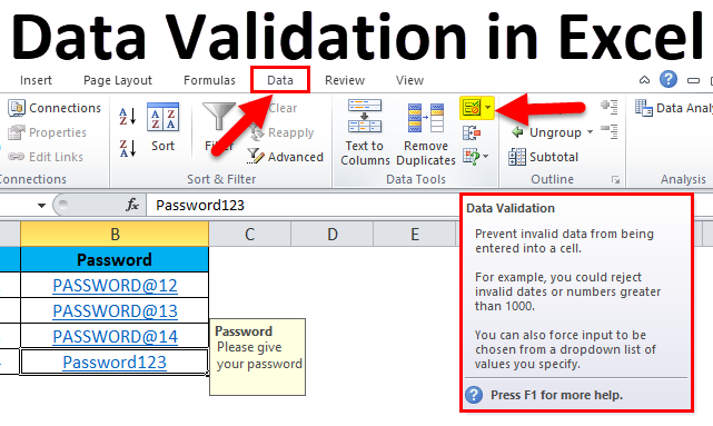
Excel Data Validation (Table of Contents)
- Data Validation in Excel
- How to Create Data Validation Rule in Excel?
- Valuation criteria of data validation Settings
Data Validation in Excel
Data validation is a feature in MS Excel used to control what a user can enter in a cell of an excel sheet. Like, restrict entries in a sheet, such as a date range or whole numbers only. We can even create dropdowns as well, which saves un-necessary space and shows the values in a single cell. Also, we can create a customized message which will appear user insert any incorrect value or an incorrect format.
As an example, A user can specify a meeting scheduled between 9:00 AM and 6:00 PM.
As we can use data validation in excel to make sure a value is a positive number, a date between 15 and 30, make sure a date occurs in the next 30 days, or make sure a text entry is less than 25 characters etc.
Locate in MS Excel
- Click on Data Tab in the Menu bar.
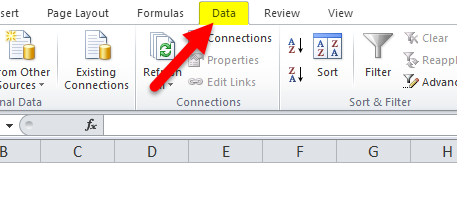
- Select on Data Validation from the toolbar under the Data Tab:
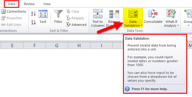
How to Create Data Validation Rule in Excel?
Let us understand the working of Data validation in excel by some examples.
You can download this Data Validation Excel Template here – Data Validation Excel Template
Example #1
We can restrict a user to enter a whole number between 0 and 10.
Execute the Below mention steps for the creation of the data validation rule in excel:
Step 1: Select B2 Cell.
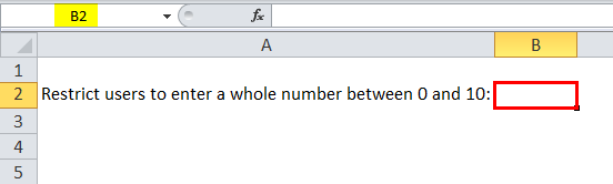
Step 2: Go to the Data tab, click on Data Validation from Data in the toolbar.
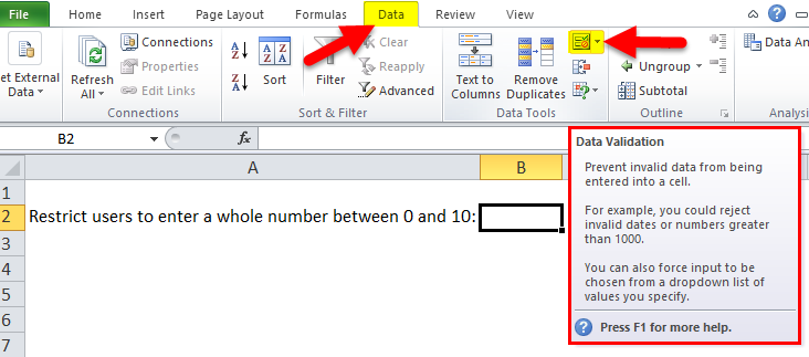
Step 3: A data validation Pop-Up will open:
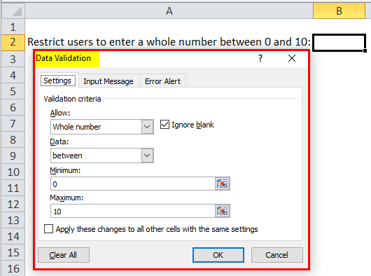
Step 3.1: On the Settings tab, Click on Allow drop-down under validation Criteria.
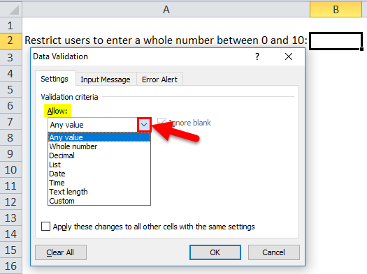
Step 3.2: Select the Whole number, then Some more required options will be enabled.
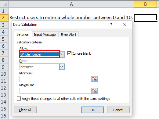
Step 3.3: Select between from the drop-down of the Data list, Enter the Minimum and Maximum number for restriction. And click ok.
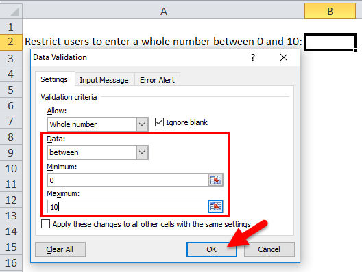
Step 3.4: All settings will apply to the selected cell.
Now Enter 1 in cell B2- It will allow a user to enter any whole number from 0 to 10.
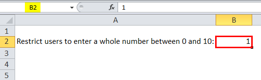
Now Enter 11 in cell B2- It will throw by default error.
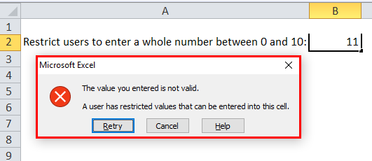
Example #2 – Set Input Message and Error Alert
We can restrict a user to enter a limited text.
Step 1: Select B5 Cell from Example 2 Sheet.
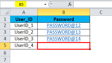
Step 2: Click on the data validation tool from the Data Menu Bar and select Text Length in Allow drop-down.
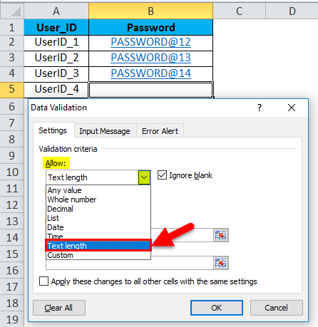
Step 3: Select equal to from the data list drop-down.
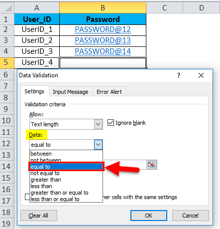
Step 4: Enter your desired length of the password (as an example 11).
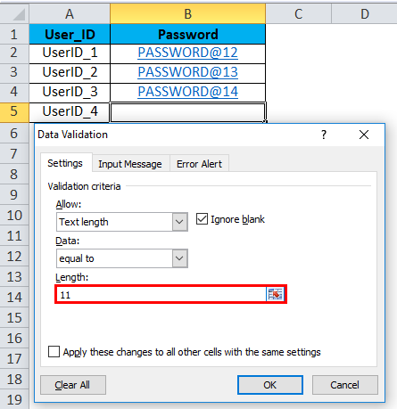
Step 5: Click on the Input Message tab and provide a message displayed on the selection of cell.
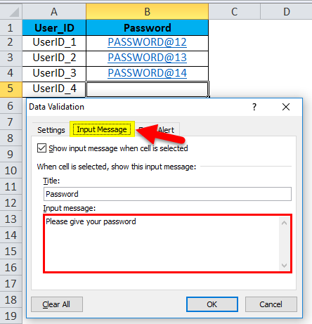
Step 6: Click on the Error Alert tab, provide a Title and the Error message, which will be displayed if a user entered an invalid length password.
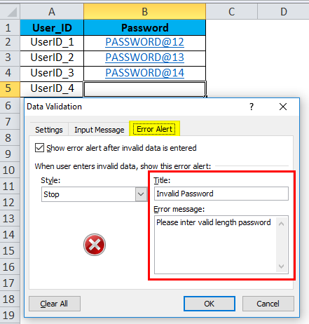
Step 7: After that, click the Ok button, the setting will be applied to the selected cell.
On the Selection of Cell, an Input message will be displayed.
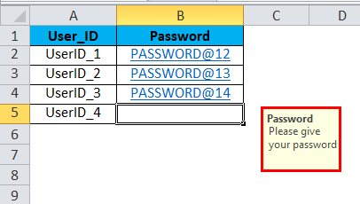
Enter a text which has a text length of 11. It will be selected successfully.
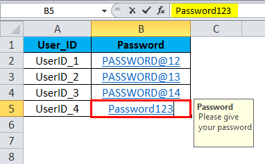
Now enter an invalid password. It will throw the described error message.
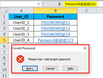
Example #3 – Custom option for e-mail address validation
Step 1: Select the C2 cell, Go to Data Tab and click on Validation data in the toolbar.
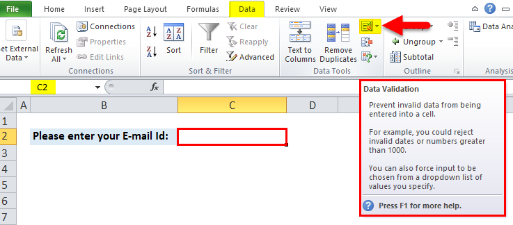
Step 2: Select custom in Allow drop-down.
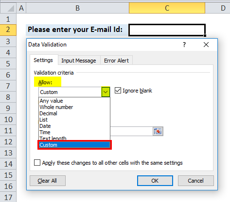
Step 3: Write a formula for selecting only value if it is having ‘@’.
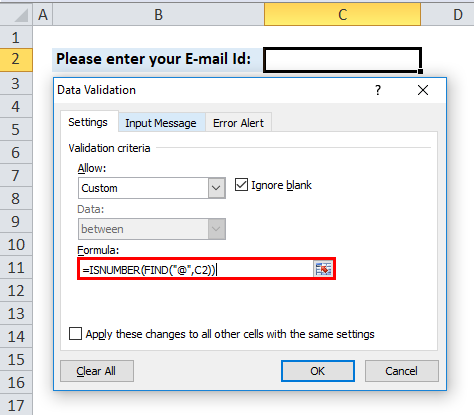
Step 4: Click on the Input Message tab, provide the message, which will be displayed on the selection of a cell.
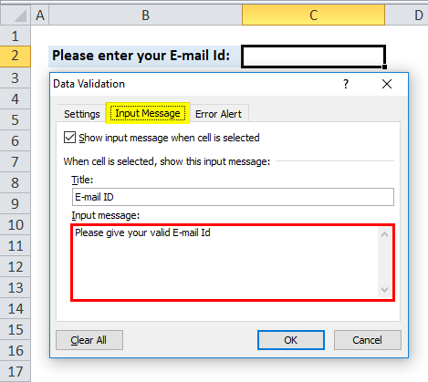
Step 5: Click on the Error Alert tab, provide the Title and an Error message, which will be displayed if a user entered an invalid length E-mail Id.
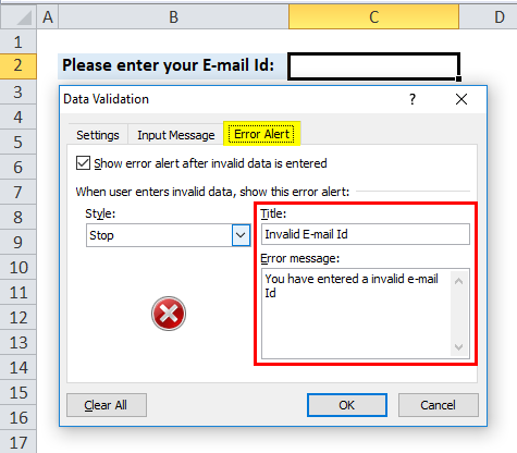
Step 6: After that, click the Ok button, the setting will be applied to the selected cell.
On the Selection of Cell, the Input message will display.
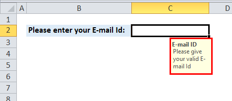
Enter a valid e-mail id – It will be selected successfully.
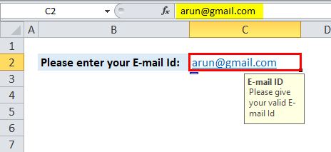
Now enter any invalid e-mail Id- It will throw a described error Message.
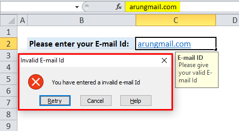
Valuation criteria of excel data validation Settings
- Any Value – To provide any type of data.
- Whole Number – Enter only whole numbers.
- Decimal – Enter only decimal numbers.
- List – Pick data from the drop-down list.
- Date – Accept the only date.
- Time – Enter only time.
- Text Length – Fixed the length of the text.
- Custom – Enter a custom formula.
Conditions in data list in Valuation criteria settings
Between, not between, equal to, not equal to, greater than, less than, greater than or equal to, less than or equal to.
Some more condition of excel data validation Settings
- If a user wants to ignore the blank, then there is a checkbox called Ignore.
- If a user selects between, then a user needs to select the Minimum and Maximum values for the cell(s).
- If a user wants to apply these changes to all other cells with the same setting, then there is a checkbox that needs to mark, and it will apply to the remaining cells in the sheet.
When to Use Data Validation in Excel?
- Best used when a user wants to share a sheet with another user, and he wants the data entered to be accurate and consistent.
- Restrict entries to predefined items in a list.
- Restrict numbers outside a specified range.
- Restrict dates outside a certain time frame.
- Restrict times outside a certain time frame.
- Limit the number of text characters.
- Validation of the data, which is available on other sheets or workbook.
- Choose to be displayed an Input Message when a user clicks on a cell as a user’s guide.
- A user can customize the error alert; it can be anything as per a user-defined.
Things to Remember About Data Validation in Excel
- If a user wants to create a data validation rule in the workbook for excel web apps or Excel services, then he needs to create an excel data validation rule on the desktop first.
- If one user sender a workbook to another, then first, a user needs to make sure that the workbook is unlocking; otherwise second, a user is never able to access the workbook cells to fill value.
- Always make in mind that there is no error in a formula like #REF! or #DIV/0!
- Anyone who can create a data validation rule in the filled cell MS excel will not detect it.
How to Remove the Excel Data Validation rule?
A user can remove excel data validation from a cell, select the cell, click Data Validation, and then click Clear All.
A user can modify or delete the excel data validation rule only if the inherited sheet is unprotected. If it is password protected, contact the owner of the workbook. Only he can help to unprotect the workbook. As there is no way to recover or lost the password option in MS Excel.
Recommended Articles
This has been a guide to Data Validation in Excel. Here we discuss how to create Data Validation in excel along with excel examples and a downloadable excel template. You may also look at these useful functions in excel –
- Excel Data Visualization
- Excel Database Template
- Excel Data Filter
- Excel Data Bars
How to Use Data Validation in Excel: Full Tutorial (2023)
Sometimes we have to share our Microsoft Excel files with multiple users to fill in data.
The problem with sharing Excel files is that other people might input the wrong data. Which in turn screws up filtering, lookups, and other types of features and functions.
To prevent this, use data validation!
And I’ll walk you through how to do that here, step-by-step, in this table😊

What is data validation in Excel?
Excel data validation helps to check input based on validation criteria. 🤔
That means data validation can be used:
- To check if a value is a number, a date, a time, a text with a specified length or
- To show a dropdown menu to the user with set options.
As a result, it can help users enter only valid data into a cell.🤗
You can also show a custom message to the user before entering data into a cell.
You can also display a warning message if the users enter invalid data.
This will simplify data entry and minimize input and typing errors. 😊
Before using Excel’s data validation feature on our table, we shall become familiar with it.👍
How to add data validation
- To start, you have to select one or more cells in the Excel file for data validation.
- Then, go to the data tab.

- Click the data validation button, in the Data Tools Group, to open the data validation settings window.
This is how the data validation window will appear.

- The first tab in the data validation window is the settings tab.
You can create rules for data validation in this tab.

For example, we can specify that the date in the first column must be a future date.
In the following part, we will go through all of the data validation rules in depth🤗.
- Go to the input message tab to create an input message.

Put a tick mark for the “Show input message when cell is selected”.

Input messages can be a guide to user input data in the correct format and reduce entering invalid data.
Add a title for the input message.

Enter a custom message for the input message.

When you select a cell with data validation, you will see an input message similar to this.

- Finally, go to the error alert tab to create an error message for invalid data.
When a user enters an invalid entry or invalid value, you can show an error alert.

Put a tick mark next to the “show error alert after invalid data is entered” in the error alert tab.

You can select 3 different styles for the error message when a user inputs invalid data.


Next, give a title to your error alert.

Then, enter a custom error message.

This error message will show up if a student enters a date that has passed.

Types of data validation rules
Dates and time validation rules
Date data validation rule
Students can make an appointment date only for a future date.
Let’s learn how to avoid entering an invalid date in the date column.
- Select “date” from the allow box in the settings tab.

By selecting “date”, restrict data entry types to date in the validation cell.
- Select a condition under the data drop down list and specify data validation criteria in the start date box.

Students can now only enter future appointment dates in the first column of the Excel table.
Time data validation rule
Next, we want to make sure that students enter appointment times between 8 a.m. and 5 p.m.
- Select “Time” as the data validation criteria from the allow box.

By selecting “Time”, all other entries other than time will become invalid entries in data validation cells.
- Select a condition under the data drop down list in the data validation dialog box.
Then enter the data validation rule for the time column.

Pro Tip!
How to change data validation settings for many cells easily?
No need to copy data validation one by one.
You can check the below box to apply the changed data validation settings to all cells with the same settings.

Number validation rules
Whole number data validation rule
We want to make sure that no more than three students attend the appointment.
In other words, we need to create an error message as invalid data if the data entry is not a whole number or is more than 3.
Let’s learn how to apply the whole number validation rule.
- Select the “Whole number” as the data validation criteria from the settings tab.

- Select a condition under data in the data validation dialog box.
I select “between” and give 1 & 3 as the minimum and maximum values.

Students can enter only 1, 2, or 3 in column C.
Decimal data validation rule
We would like to get the group results when they are scheduling the appointment.
The results should be between 0% to 100% (i.e., the results should be between 0 to 1).
Let’s learn how to do data validation in excel for decimal values.
- Select “Decimal” as the data validation criteria from the settings tab.

- Select a condition from the list under data and apply validation criteria.

Text validation rule
Do you think we can have data validation in Excel only for numeric values?🤔
No. We can apply for data validation in excel for text length as well.
When the user inputs a text that has a different length to the given data validation that data entry can be recognized as invalid data.
In this table, the group name should be less than 15 letters.
Let’s look at how we can validate the group name.
- Select the “Text length” as the data validation criteria from the settings tab.

- Select a condition for the data validation from the data box.

Drop-down lists
In the last column, students must enter either “Batch 1” or “Batch 2”.
We can give those 2 options in a cell dropdown box.
If the user selects “Batch 1”, it will show in that cell.
Let’s learn how to create a drop down list.
- Select the “List” as the data validation criteria.

- Enter the items for the drop down list in the source box or give a specified range for the drop down list in the source box.
To give a cell reference, click the upside arrow in the source box.

Pro Tip!
Is it difficult to update drop down list, if the number of options for drop down list are changing every time?😕
Don’t worry.
Give the cell reference of the source box to a Table in Excel.
The table automatically updates your list.😍
With the drop down list, users can easily select the batch.

Since drop down list is a very common data validation feature, it is good to learn this in a very detailed manner.
Check our https://spreadsheeto.com/drop-down/ article to quickly learn more about Excel drop down lists.
Now users can enter only valid entries into our Excel table.
How to remove data validation
Now you know how to apply data validation in excel.👏
Do you want to know how to remove data validation?
It is very simple!🙂
- Select the cells that contain data validation you need to remove.
- Go to the data tab
- Click on the data validation icon.
- Click “Clear All”.

That’s it – Now what?
Now, you can easily add data validation to your cells, making it almost impossible for other users to mess up data input 😊
Pretty great, right?
But messed up data is only a problem if there’s something relying on that data.
Functions like IF, SUMIF, and VLOOKUP rely on data being neat and orderly. And those functions are the backbone of most important spreadsheets.
If you don’t master them yet, click here to learn IF, SUMIF, and VLOOKUP in my free 30-minute online course.
Other resources
If you want to use more advanced date and time functions as validation conditions, read our article about Excel’s Date and Time Functions.
After applying data validation, it is quite simple to narrow down your data to find what is relevant with Excel Filters. Read our How to Filter in Excel article to find out more information about the Excel filter tool.
And not just that! When you have complete data, you can easily rearrange it using Pivot Tables.
Kasper Langmann2023-02-23T11:33:26+00:00
Page load link
You can help users enter accurate and appropriate information into your worksheets with Excel’s Data Validation feature. Data validation restricts the type of information that can be entered in a cell and can provide the user with instructions for entering information in a cell.
Create a Validation Rule
- Select the cells you want to validate.
- Click the Data tab.
- Click the Data Validation button.

- Click the Allow list arrow.
- Select the type of data you want to allow.
- Any value: No validation criteria applied.
- Whole number: Allows a whole number between the minimum and maximum limits set.
- Decimal: Allows a decimal or a percent entered as a decimal between the set limits.
- List: Allows a value from a list of choices. A list arrow appears in the cell, and users can choose from the list.
- Date: Allows a date within set limits.
- Time: Allows a time within set limits.
- Text length: Allows text containing a certain number of characters.
- Custom: Allows a formula to be entered to calculate what is allowed in the cell.
- Specify the data validation rules.
The validation options will vary depending on the option selected in the Allow field.
- Click OK.
The data validation is set for the selected cell(s). When a user tries to enter data that is not valid, Excel will prevent the entry and display a message about the cell being restricted.
To find validated data in a worksheet, click the Find & Select button in the Editing group on the Home tab and select Data Validation. The validated cells are highlighted.
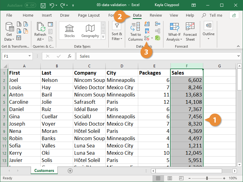
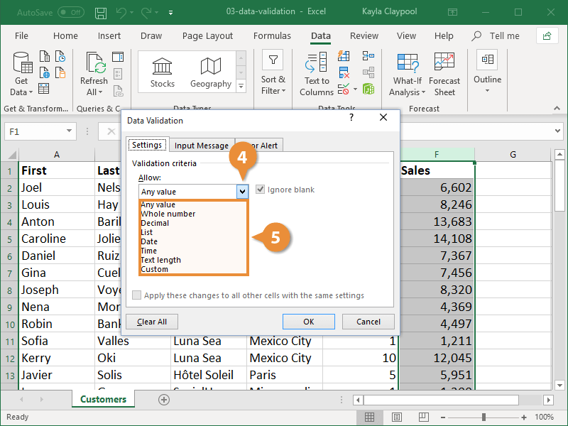
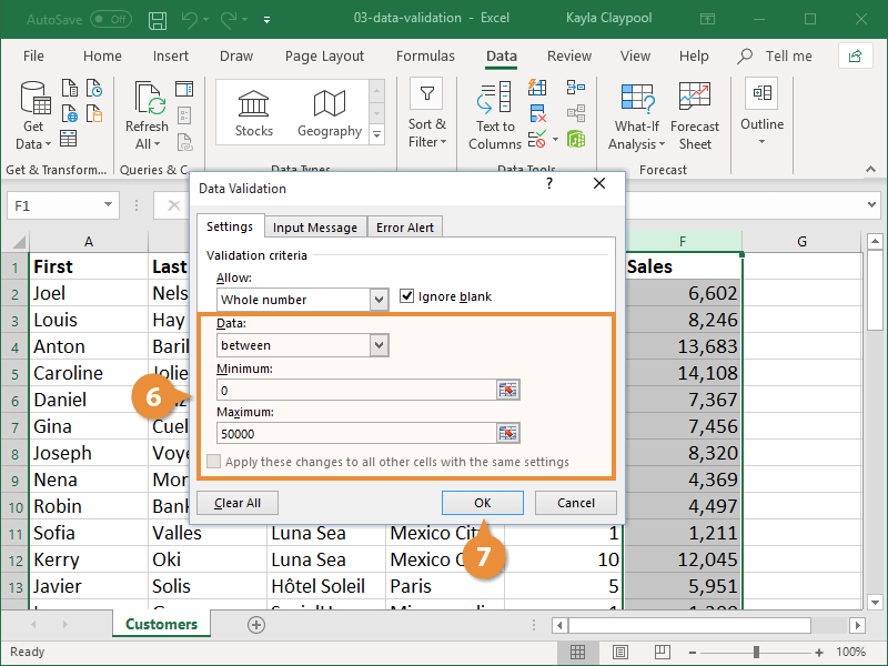
Add Input and Error Messages
Prevent data validation issues by setting up Excel to display a message whenever a cell or range of cells is selected. These messages are useful when other people will be entering data in your worksheet. An error message can be configured to appear when data is entered that does not match a data validation rule.
- Select the cells where you want an input message to appear.
- Click the Data tab.
- Click the Data Validation button.
- Click the Input Message tab.
- Enter an input message.
- Click the Error Alert tab.
- Select an error alert style.
- Stop: Prevents users from adding invalid data in a cell.
- Warning: Warns that the data entered is invalid, but users can click Yes to accept the invalid entry, No to edit it, or Cancel to remove it.
- Information: Informs users that the data entered is invalid, but users can click OK to accept the invalid entry or Cancel to remove it.
- Enter an error alert message.
- Click OK.
- Select a cell with an input message.
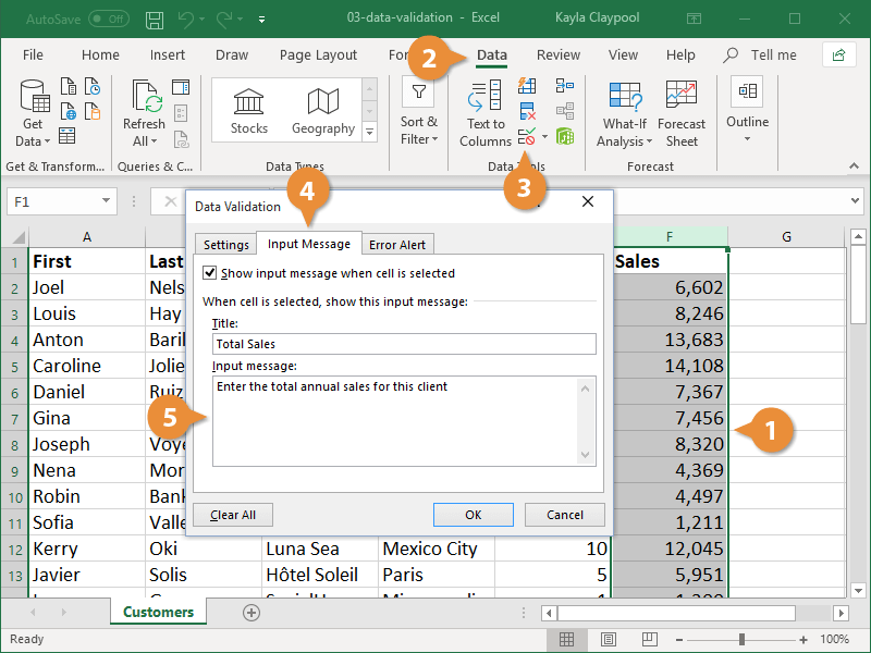
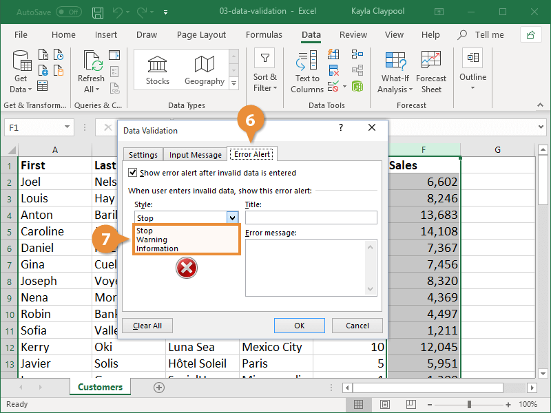
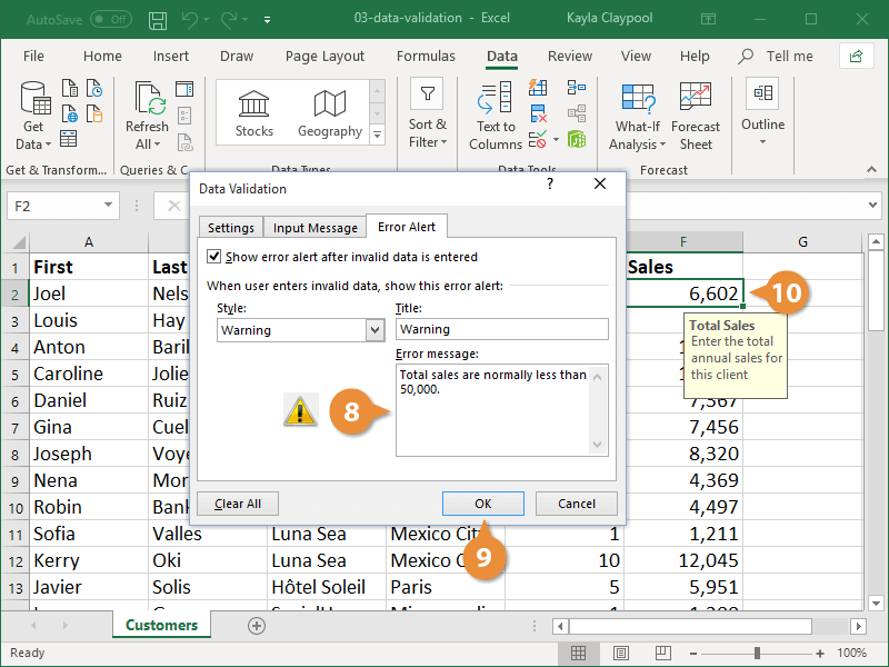
Now when a cell in the range is selected, the title and message display. If you enter an invalid value, a custom error message appears.

FREE Quick Reference
Click to Download
Free to distribute with our compliments; we hope you will consider our paid training.