Using where in excel

How to Return Cell Address Instead of Value in Excel (Easy Formula)

When using lookup formulas in Excel (such as VLOOKUP, XLOOKUP, or INDEX/MATCH), the intent is to find the matching value and get that value (or a corresponding value in the same row/column) as the result.

But in some cases, instead of getting the value, you may want the formula to return the cell address of the value.

This could be especially useful if you have a large data set and you want to find out the exact position of the lookup formula result.

There are some functions in Excel that designed to do exactly this.

In this tutorial, I will show you how you can find and return the cell address instead of the value in Excel using simple formulas.

This Tutorial Covers:

Lookup And Return Cell Address Using the ADDRESS Function

The ADDRESS function in Excel is meant to exactly this.

It takes the row and the column number and gives you the cell address of that specific cell.

Below is the syntax of the ADDRESS function:

• row_num: Row number of the cell for which you want the cell address
• column_num: Column number of the cell for which you want the address
• [abs_num]: Optional argument where you can specify whether want the cell reference to be absolute, relative, or mixed.
• [a1]: Optional argument where you can specify whether you want the reference in the R1C1 style or A1 style
• [sheet_text]: Optional argument where you can specify whether you want to add the sheet name along with the cell address or not

Now, let’s take an example and see how this works.

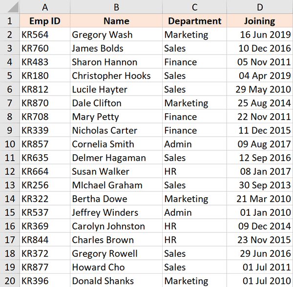
Suppose there is a dataset as shown below, where I have the Employee id, their name, and their department, and I want to quickly know the cell address that contains the department for employee id KR256.

Below is the formula that will do this:

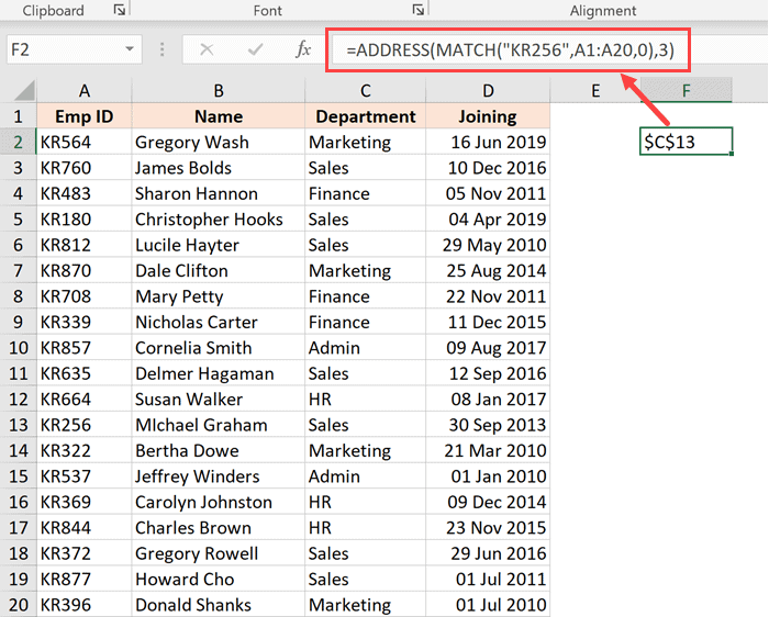
In the above formula, I have used the MATCH function to find out the row number that contains the given employee id.

And since the department is in column C, I have used 3 as the second argument.

This formula works great, but it has one drawback – it won’t work if you add the row above the dataset or a column to the left of the dataset.

This is because when I specify the second argument (the column number) as 3, it’s hard-coded and won’t change.

In case I add any column to the left of the dataset, the formula would count 3 columns from the beginning of the worksheet and not from the beginning of the dataset.

So, if you have a fixed dataset and need a simple formula, this will work fine.

But if you need this to be more fool-proof, use the one covered in the next section.

Lookup And Return Cell Address Using the CELL Function

While the ADDRESS function was made specifically to give you the cell reference of the specified row and column number, there is another function that also does this.

It’s called the CELL function (and it can give you a lot more information about the cell than the ADDRESS function).

Below is the syntax of the CELL function:

• info_type: the information about the cell you want. This could be the address, the column number, the file name, etc.
• [reference]: Optional argument where you can specify the cell reference for which you need the cell information.

Now, let’s see an example where you can use this function to look up and get the cell reference.

Suppose you have a dataset as shown below, and you want to quickly know the cell address that contains the department for employee id KR256.

Below is the formula that will do this:

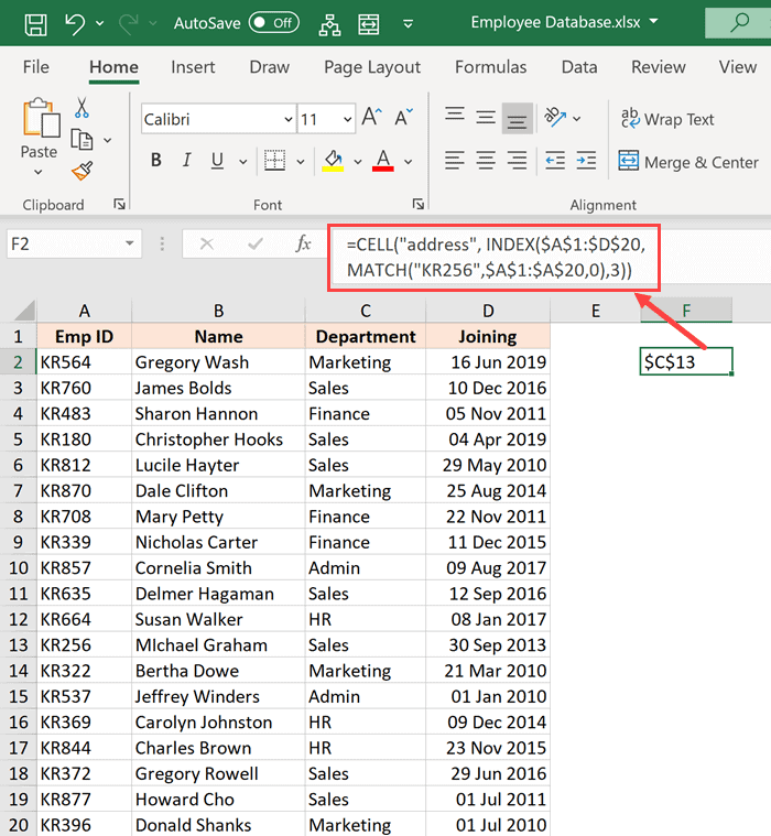
The above formula is quite straightforward.

I have used the INDEX formula as the second argument to get the department for the employee id KR256.

And then simply wrapped it within the CELL function and asked it to return the cell address of this value that I get from the INDEX formula.

Now here is the secret to why it works – the INDEX formula returns the lookup value when you give it all the necessary arguments. But at the same time, it would also return the cell reference of that resulting cell.

In our example, the INDEX formula returns “Sales” as the resulting value, but at the same time, you can also use it to give you the cell reference of that value instead of the value itself.

Normally, when you enter the INDEX formula in a cell, it returns the value because that is what it’s expected to do. But in scenarios where a cell reference is required, the INDEX formula will give you the cell reference.

In this example, that’s exactly what it does.

And the best part about using this formula is that it is not tied to the first cell in the worksheet. This means that you can select any data set (which could be anywhere in the worksheet), use the INDEX formula to do a regular look up and it would still give you the correct address.

And if you insert an additional row or column, the formula would adjust accordingly to give you the correct cell address.

So these are two simple formulas that you can use to look up and find and return the cell address instead of the value in Excel.

I hope you found this tutorial useful.

Other Excel tutorials you may also like:

Источник

Search Function in Excel

Excel SEARCH Function

The SEARCH function in Excel is categorized under text or string functions, but the output returned by this function is an integer. The SEARCH function gives us the position of a substring in a given string when we provide a parameter of the position to search from. Thus, this formula takes three arguments: substring, the string itself, and position to start the search.

For example, suppose we want to search the “Thank” substring in the provided text or string “Thank you.” Here, we need to find the “Thank” word using the SEARCH function, which will return the word “Thank” location.

=SEARCH(“Thank,” B8). The output will be 1.

The SEARCH function is a text function used to find the location of a substring in a string/text.

The SEARCH function can be used as a worksheet function. It is not case-sensitive.

Table of contents

SEARCH Formula in Excel

Below is the SEARCH formula in Excel.

Explanation

Excel SEARCH function has three-parameter two (find_text, within_text) are compulsory parameters and one (start_num) is optional.

Compulsory Parameter:

• find_text: find_text refers to the substring/character you want to search within a string or the text you want to find out.
• within_text:. Where your substring is located or where you perform the find_text.

Optional Parameter:

How to Use the Search Function in excel? (with Examples)

The SEARCH function is very simple and easy to use. Let us understand the working of the SEARCH function in some examples.

Example #1

Let us search the “Good” substring in the given text or string. Here, we have found the “Good” word using the SEARCH function, which will return the word “Good” location in the “Good morning.”

=SEARCH(“Good,” B6) and output will be 1.

Suppose two matches are found for “Good,” then SEARCH in Excel will give you the first match value. However, if you want the other good location, then you use the =SEARCH(“Good,” B7, 2) [start_num] as 2 then it will give you the place of the second match value, and the output will be 6.

Example #2

For first name=LEFT(B12,SEARCH(” “,B12)-1)

For last name=RIGHT(B12,LEN(B12)-SEARCH(” “,B12))

Example #3

Suppose there is a set of IDs. First, you have to find the _ location within IDs, then use Excel SEARCH to find the “_” location within IDs.

=SEARCH(“_,” B27), and output will be 6.

Example #4

Consider the table and search for the next 0 within the text A1-001-ID.

And start position will be 1, then =SEARCH(“?” &I8, J8, K8) output will be 3 because “?” neglects the one character before the 0, and output will be 3.

For the second row within a given table, the search result for A within B1-001-AY.

It will be 8, but if we use “*” in search, it will give you the 1 as location output because it will neglect all characters before “A,” and output will be 1 for it =SEARCH(“*” &I9, J9).

Similarly, for “J” 8 =SEARCH(I10,J10,K10) and 7 for =SEARCH(“?”&I10,J10,K10).

Similarly, for fourth row, the output will be 8 for =SEARCH(I11,J11,K11) and 1 for =SEARCH(“*” &I11,J11,K11)

Things to Remember

• It is not case-sensitive.
  • It considers tanuj and TANUJ as the same value, which means it does not distinguish between lower and upper case.
• It is also allowed wildcard characters, i.e., “?”, “*,” and “

  ” tilde.

  • “?” is used to find a single character.
  • “*” is used for match sequences.
  • If we want to search the “*” or”? “, we need to insert the “

    ” before the character.

• It returns the #VALUE! Error if there is no matching string is found in the within_text.

Suppose in the below example. We are searching for a substring “a” within the “Name” column. If found, it will return the location of a within name else. In addition, it will give a #VALUE error #VALUE Error #VALUE! Error in Excel represents that the reference cell the user has either entered an incorrect formula or used a wrong data type (mostly numerical data). Sometimes, it is difficult to identify the kind of mistake behind this error. read more , as shown below.

Search Function in Excel Video

Recommended Articles

This article is a guide to the SEARCH Function in Excel. Here, we discuss the SEARCH formula and how to use the SEARCH function, along with Excel examples and downloadable Excel templates. You may also look at these useful functions in Excel: –

Источник

Thanks. We have received your request and will respond promptly.

Come Join Us!

• Talk With Other Members
• Be Notified Of Responses
  To Your Posts
• Keyword Search
• One-Click Access To Your
  Favorite Forums
• Automated Signatures
  On Your Posts
• Best Of All, It’s Free!

Posting Guidelines

Promoting, selling, recruiting, coursework and thesis posting is forbidden.

USING THE ‘WHERE’ CLAUSE IN EXCEL

USING THE ‘WHERE’ CLAUSE IN EXCEL

USING THE ‘WHERE’ CLAUSE IN EXCEL

New to the forum, can anyone tell me how I can use the where clause in a cell in excel. I have another sheet and a column called rowid. I would like to use this rule

SUMTOTAL OF CELLS WHERE ROWID = 21

Thxs in advance

RE: USING THE ‘WHERE’ CLAUSE IN EXCEL

Three things are certain. Death, taxes and lost data. DPlank is to blame

Please read FAQ222-2244 before you ask a question

RE: USING THE ‘WHERE’ CLAUSE IN EXCEL

RE: USING THE ‘WHERE’ CLAUSE IN EXCEL

Three things are certain. Death, taxes and lost data. DPlank is to blame

Please read FAQ222-2244 before you ask a question

RE: USING THE ‘WHERE’ CLAUSE IN EXCEL

RE: USING THE ‘WHERE’ CLAUSE IN EXCEL

A B
1 Property Value Commission
2 100,000 7,000
3 200,000 14,000
4 300,000 21,000
5 400,000 28,000

Formula Description (Result)
=SUMIF(A2:A5,»>160000″,B2:B5) Sum of the commissions for property values over 160000 (63,000)

Three things are certain. Death, taxes and lost data. DPlank is to blame

Please read FAQ222-2244 before you ask a question

RE: USING THE ‘WHERE’ CLAUSE IN EXCEL

Well I have a mixture of ids, on each case I would search on a criteria

IE: Equal to 21 for one row
equal to 31 for another, the sheet is a mixture of rowids so only certain ids ie: == 21 for one row in another sheet would apply, hope this makes sense

RE: USING THE ‘WHERE’ CLAUSE IN EXCEL

Rather than speaking in riddles, please state your requrements in a clear, concise manner.

Skip,

_{Be advised: To be safe on the FOURTH, don’t take a FIFTH on the THIRD, or.
You might not come FORTH on the FIFTH!}

RE: USING THE ‘WHERE’ CLAUSE IN EXCEL

Sum of the values in B2:B100 WHERE the corresponding rowID in A2:A100 is 21 (Assuming 21 is numeric)

If the 21 is not numeric then it must be enclosed in quotes within the formula, eg

If you have a list of IDs in your spreadsheet in say cells J1:J5, and you wish to use this formula against each of those IDs in the list, then you can substitute the 21 or «21» for a cell reference, so in say K1 simply put the formula

and then copy down to K5. Note that the row part of the references have been made absolute with the use of the $ signs so that they don’t change when you copy down.

If this doesn’t help either then you need to give an example of your data, state what you want to get out of it, and give us the answer you would expect from the data you provide.

If you wish to sum on more than one criteria then investigate the SUMPRODUCT function in Help.

—————————————————————————-
It’s easier to beg forgiveness than ask permission
—————————————————————————-

RE: USING THE ‘WHERE’ CLAUSE IN EXCEL

RE: USING THE ‘WHERE’ CLAUSE IN EXCEL

Need help finding an answer?

Try the Search Facility or read FAQ222-2244 on how to get better results.

RE: USING THE ‘WHERE’ CLAUSE IN EXCEL

RE: USING THE ‘WHERE’ CLAUSE IN EXCEL

Give us the EXACT formulas you used when you tried it in the same sheet and also when you tried it against a different sheet. Don’t type them out, actually go into the cell and copy the formulas themselves and then paste into your note.

—————————————————————————-
It’s easier to beg forgiveness than ask permission
—————————————————————————-

RE: USING THE ‘WHERE’ CLAUSE IN EXCEL

RE: USING THE ‘WHERE’ CLAUSE IN EXCEL

—————————————————————————-
It’s easier to beg forgiveness than ask permission
—————————————————————————-

Red Flag Submitted

Thank you for helping keep Tek-Tips Forums free from inappropriate posts.
The Tek-Tips staff will check this out and take appropriate action.

Reply To This Thread

Posting in the Tek-Tips forums is a member-only feature.

Click Here to join Tek-Tips and talk with other members! Already a Member? Login

Источник