
Excel for Microsoft 365 Excel for Microsoft 365 for Mac Excel 2021 Excel 2021 for Mac Excel 2019 Excel 2019 for Mac Excel 2016 Excel 2016 for Mac Excel 2013 Excel 2010 Excel 2007 Excel for Mac 2011 More…Less
By using What-If Analysis tools in Excel, you can use several different sets of values in one or more formulas to explore all the various results.
For example, you can do What-If Analysis to build two budgets that each assumes a certain level of revenue. Or, you can specify a result that you want a formula to produce, and then determine what sets of values will produce that result. Excel provides several different tools to help you perform the type of analysis that fits your needs.
Note that this is just an overview of those tools. There are links to help topics for each one specifically.
What-If Analysis is the process of changing the values in cells to see how those changes will affect the outcome of formulas on the worksheet.
Three kinds of What-If Analysis tools come with Excel: Scenarios, Goal Seek, and Data Tables. Scenarios and Data tables take sets of input values and determine possible results. A Data Table works with only one or two variables, but it can accept many different values for those variables. A Scenario can have multiple variables, but it can only accommodate up to 32 values. Goal Seek works differently from Scenarios and Data Tables in that it takes a result and determines possible input values that produce that result.
In addition to these three tools, you can install add-ins that help you perform What-If Analysis, such as the Solver add-in. The Solver add-in is similar to Goal Seek, but it can accommodate more variables. You can also create forecasts by using the fill handle and various commands that are built into Excel.
For more advanced models, you can use the Analysis ToolPak add-in.
A Scenario is a set of values that Excel saves and can substitute automatically in cells on a worksheet. You can create and save different groups of values on a worksheet and then switch to any of these new scenarios to view different results.
For example, suppose you have two budget scenarios: a worst case and a best case. You can use the Scenario Manager to create both scenarios on the same worksheet, and then switch between them. For each scenario, you specify the cells that change and the values to use for that scenario. When you switch between scenarios, the result cell changes to reflect the different changing cell values.
1. Changing cells
2. Result cell
1. Changing cells
2. Result cell
If several people have specific information in separate workbooks that you want to use in scenarios, you can collect those workbooks and merge their scenarios.
After you have created or gathered all the scenarios that you need, you can create a Scenario Summary Report that incorporates information from those scenarios. A scenario report displays all the scenario information in one table on a new worksheet.
Note: Scenario reports are not automatically recalculated. If you change the values of a scenario, those changes will not show up in an existing summary report. Instead, you must create a new summary report.
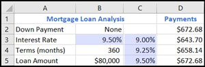
If you know the result that you want from a formula, but you’re not sure what input value the formula requires to get that result, you can use the Goal Seek feature. For example, suppose that you need to borrow some money. You know how much money you want, how long a period you want in which to pay off the loan, and how much you can afford to pay each month. You can use Goal Seek to determine what interest rate you must secure in order to meet your loan goal.

Cells B1, B2, and B3 are the values for the loan amount, term length, and interest rate.
Cell B4 displays the result of the formula =PMT(B3/12,B2,B1).
Note: Goal Seek works with only one variable input value. If you want to determine more than one input value, for example, the loan amount and the monthly payment amount for a loan, you should instead use the Solver add-in. For more information about the Solver add-in, see the section Prepare forecasts and advanced business models, and follow the links in the See Also section.
If you have a formula that uses one or two variables, or multiple formulas that all use one common variable, you can use a Data Table to see all the outcomes in one place. Using Data Tables makes it easy to examine a range of possibilities at a glance. Because you focus on only one or two variables, results are easy to read and share in tabular form. If automatic recalculation is enabled for the workbook, the data in Data Tables immediately recalculates; as a result, you always have fresh data.
Cell B3 contains the input value.
Cells C3, C4, and C5 are values Excel substitutes based on the value entered in B3.
A Data Table cannot accommodate more than two variables. If you want to analyze more than two variables, you can use Scenarios. Although it is limited to only one or two variables, a Data Table can use as many different variable values as you want. A Scenario can have a maximum of 32 different values, but you can create as many scenarios as you want.
If you want to prepare forecasts, you can use Excel to automatically generate future values that are based on existing data, or to automatically generate extrapolated values that are based on linear trend or growth trend calculations.
You can fill in a series of values that fit a simple linear trend or an exponential growth trend by using the fill handle or the Series command. To extend complex and nonlinear data, you can use worksheet functions or the regression analysis tool in the Analysis ToolPak Add-in.
Although Goal Seek can accommodate only one variable, you can project backward for more variables by using the Solver add-in. By using Solver, you can find an optimal value for a formula in one cell—called the target cell—on a worksheet.
Solver works with a group of cells that are related to the formula in the target cell. Solver adjusts the values in the changing cells that you specify—called the adjustable cells—to produce the result that you specify from the target cell formula. You can apply constraints to restrict the values that Solver can use in the model, and the constraints can refer to other cells that affect the target cell formula.
Need more help?
You can always ask an expert in the Excel Tech Community or get support in the Answers community.
See Also
Scenarios
Goal Seek
Data Tables
Using Solver for capital budgeting
Using Solver to determine the optimal product mix
Define and solve a problem by using Solver
Analysis ToolPak Add-in
Overview of formulas in Excel
How to avoid broken formulas
Detect errors in formulas
Keyboard shortcuts in Excel
Excel functions (alphabetical)
Excel functions (by category)
Need more help?
Want more options?
Explore subscription benefits, browse training courses, learn how to secure your device, and more.
Communities help you ask and answer questions, give feedback, and hear from experts with rich knowledge.
What is IF Function in Excel?
IF function in Excel evaluates whether a given condition is met and returns a value depending on whether the result is “true” or “false”. It is a conditional function of Excel, which returns the result based on the fulfillment or non-fulfillment of the given criteria.
For example, the IF formula in Excel can be applied as follows:
“=IF(condition A,“value B”,“value C”)”
The IF excel function returns “value B” if condition A is met and returns “value C” if condition A is not met.
It is often used to make logical interpretations which help in decision-making.
Table of contents
- What is IF Function in Excel?
- Syntax of the IF Excel Function
- How to Use IF Function in Excel?
- Example #1
- Example #2
- Example #3
- Example #4
- Example #5
- Guidelines for the Multiple IF Statements
- Frequently Asked Question
- IF Excel Function Video
- Recommended Articles
Syntax of the IF Excel Function
The syntax of the IF function is shown in the following image:

The IF excel function accepts the following arguments:
- Logical_test: It refers to the condition to be evaluated. The condition can be a value or a logical expression.
- Value_if_true: It is the value returned as a result when the condition is “true”.
- Value_if_false: It is the value returned as a result when the condition is “false”.
In the formula, the “logical_test” is a required argument, whereas the “value_if_true” and “value_if_false” are optional arguments.
The IF formula uses logical operators to evaluate the values in a range of cells. The following table shows the different logical operatorsLogical operators in excel are also known as the comparison operators and they are used to compare two or more values, the return output given by these operators are either true or false, we get true value when the conditions match the criteria and false as a result when the conditions do not match the criteria.read more and their meaning.
| Operator | Meaning |
|---|---|
| = | Equal to |
| > | Greater than |
| >= | Greater than or equal to |
| < | Less than |
| <= | Less than or equal to |
| <> | Not equal to |
How to Use IF Function in Excel?
Let us understand the working of the IF function with the help of the following examples in Excel.
You can download this IF Function Excel Template here – IF Function Excel Template
Example #1
If there is no oxygen on a planet, life is impossible. If oxygen is available on a planet, then life is possible. The following table shows a list of planets in column A and the information on the availability of oxygen in column B. We have to find the planets where life is possible, based on the condition of oxygen availability.

Let us apply the IF formula to cell C2 to find out whether life is possible on the planets listed in the table.
The IF formula is stated as follows:
“=IF(B2=“Yes”, “Life is Possible”, “Life is Not Possible”)
The succeeding image shows the IF formula applied to cell C2.

The subsequent image shows how the IF formula is applied to the range of cells C2:C5.

Drag the cells to view the output of all the planets.

The output in the below worksheet shows life is possible on the planet Earth.
Flow Chart of Generic IF Excel Function

The IF Function Flow Chart for Mars (Example #1)

The flow of IF function flowchart for Jupiter and Venus is the same as the IF function flowchart for Mars (Example #1).
The IF Function Flow Chart for Earth

Hence, the IF excel function allows making logical comparisons between values. The modus operandi of the IF function is stated as: If something is true, then do something; otherwise, do something else.
Example #2
The following table shows a list of years. We want to find out if the given year is a leap year or not.
A leap year has 366 days; the extra day is the 29th of February. The criteria for a leap year are stated as follows:
- The year will be exactly divisible by 4 and not exactly be divisible by 100 or
- The year will be exactly divisible by 400.

In this example, we will use the IF function along with the AND, OR, and MOD functions to find the leap years.
We use the MOD function to find a remainder after a dividend is divided by a divisor.
The AND functionThe AND function in Excel is classified as a logical function; it returns TRUE if the specified conditions are met, otherwise it returns FALSE.read more evaluates both the conditions of the leap years for the value “true”. The OR functionThe OR function in Excel is used to test various conditions, allowing you to compare two values or statements in Excel. If at least one of the arguments or conditions evaluates to TRUE, it will return TRUE. Similarly, if all of the arguments or conditions are FALSE, it will return FASLE.read more evaluates either of the condition for the value “true”.
We will apply the MOD function to the conditions as follows:
If MOD(year,4)=0 and MOD(year,100)<>(is not equal to) 0, then the year is a leap year.
or
If MOD(year,400)=0, then the year is a leap year; otherwise, the year is not a leap year.
The IF formula is stated as follows:
“=IF(OR(AND((MOD(year,4)=0),(MOD(year,100)<>0)),(MOD(year,400)=0)),“Leap Year”, “Not A Leap Year”)”
The argument “year” refers to a reference value.
The following images show the output of the IF formula applied in the range of cells.


The following image shows how the IF formula is applied to the range of cells B2:B18.

The succeeding table shows the years 1960, 2028, and 2148 as leap years and the remaining as non-leap years.

The result of the IF excel formula is displayed for the range of cells B2:B18 in the following image.

Example #3
The succeeding table shows a list of drivers and the directions they undertook to reach the destination. It is preceded by an image of the road intersection explaining the turns taken by the drivers and their destinations. The right turn leads to town B, and the left turn leads to town C. Identify the driver’s destination to town B and town C.
Road Intersection Image


Let us apply the IF excel function to find the destination. Here, the condition is mentioned as follows:
- If the driver turns right, he/she reaches town B.
- If the driver turns left, he/she reaches town C.
We use the following IF formula to find the destination:
“=IF(B2=“Left”, “Town C”, “Town B”)”
The succeeding image shows the output of the IF formula applied to cell C2.

Drag the cells to use the formula in the range C2:C11. Finally, we get the destinations of each driver for their turning movements.
The below image displays the IF formula applied to the range.

The output of the IF formula and the destinations are displayed in the succeeding image.

The result shows that six drivers reached town C, and the remaining four have reached town B.
Example #4
The following table shows a list of items and their inventory levels. We want to check if the specific item is available in the inventory or not using the IF function.

Let us list the name of items in column A and the number of items in column B. The list of data to be validated for the entire items list is shown in the cell E2 of the below image.

We use the Excel IF along with the VLOOKUP functionThe VLOOKUP excel function searches for a particular value and returns a corresponding match based on a unique identifier. A unique identifier is uniquely associated with all the records of the database. For instance, employee ID, student roll number, customer contact number, seller email address, etc., are unique identifiers.
read more to check the availability of the items in the inventory.
The VLOOKUP function looks up the values referring to the number of items, and the IF function will check whether the item number is greater than zero or not.
We will apply the following IF formula in the F2 cell:
“=IF(VLOOKUP(E2,A2:B11,2,0)=0, “Item Not Available”,“Item Available”)”
If the lookup value of an item is equal to 0, then the item is not available; else, the item is available.
The succeeding image shows the result of the IF formula in the cell F2.

Select “bat” in the E2 item cell to know whether the item is available or not in the inventory (as shown in the following image).

Example #5
The following table shows the list of students and their marks. The grade criteria are provided based on the marks obtained by the students. We want to find the grade of each student in the list.

We apply the Nested IF in Excel since we have multiple criteria to find and decide each student’s grade.
The Nesting of IF function uses the IF function inside another IF formula when multiple conditions are to be fulfilled.
The syntax of Nesting of IF function is stated as follows:
“=IF( condition1, value_if_true1, IF( condition2, value_if_true2, value_if_false2 ))”
The succeeding table represents the range of scores and the grades, respectively.

Let us apply the multiple IF conditions with AND function in the below-nested formula to find out the grade of the students:
“=IF((B2>=95),“A”,IF(AND(B2>=85,B2<=94),“B”,IF(AND(B2>=75,B2<=84),“C”,IF(AND(B2>=61,B2<=74),“D”,“F”))))”
The IF function checks the logical condition as shown in the formula below:
“=IF(logical_test, [value_if_true],[value_if_false])”
We will split the above-mentioned nested formula and check the IF statements as shown below:
First Logical Test: B2>=95
If the formula returns,
- Value_if_true, execute: “A” (Grade A) else(comma) enter value_if_false
- Value_if_false, then the formula finds another IF condition and enter IF condition
Second Logical Test: B2>=85(logical expression 1) and B2<=94(logical expression 2)
(We use AND function to check the multiple logical expressions as the two given conditions are to be evaluated for “true.”)
If the formula returns,
- Value_if_true, execute: “B” (Grade B) else(comma) enter value_if_false
- Value_if_false, then the formula finds another IF condition and enter IF condition
Third Logical Test: B2>=75(logical expression 1) and B2<=84(logical expression 2)
(We use AND function to check the multiple logical expressions as the two given conditions are to be evaluated for “true.”)
If the formula returns,
- Value_if_true, execute: “C” (Grade C) else(comma) enter value_if_false
- value_if_false, then the formula finds another IF condition and enter IF condition
Fourth Logical Test: B2>=61(logical expression 1) and B2<=74(logical expression 2)
(We use AND function to check the multiple logical expressions as the two given conditions are to be evaluated for “true.”)
If the formula returns,
- Value_if_true, execute: “D” (Grade D) else(comma) enter value_if_false
- Value_if_false, execute: “F” (Grade F)
- Finally, close the parenthesis.
The below image displays the output of the IF formula applied to the range.

The succeeding image shows the IF nested formula applied to the range.

The grades of the students are listed in the following table.

Guidelines for the Multiple IF Statements
The guidelines for the multiple IF statements are listed as follows:
- Use nested IF function to a limited extent as multiple IF statements require a great deal of thought to be accurate.
- Multiple IF statementsIn Excel, multiple IF conditions are IF statements that are contained within another IF statement. They are used to test multiple conditions at the same time and return distinct values. Additional IF statements can be included in the ‘value if true’ and ‘value if false’ arguments of a standard IF formula.read more require multiple parentheses (), which is often difficult to manage. Excel provides a way to check the color of each opening and closing parenthesis to avoid this situation. The last closing parenthesis color will always be black, denoting the end of the formula statement.
- Whenever we pass a string value for the arguments “value_if_true” and “value_if_false” or test a reference against a string value, enclose the string value in double quotes. Passing a string value without quotes will result in “#NAME?” error.
Frequently Asked Question
1. What is the IF function in Excel?
The Excel IF function is a logical function that checks the given criteria and returns one value for a “true” and another value for a “false” result.
The syntax of the IF function is stated as follows:
“=IF(logical_test, [value_if_true], [value_if_false])”
The arguments are as follows:
1. Logical_test – It refers to a value or condition that is tested.
2. Value_if_true – It is the value returned when the condition logical_test is “true.”
3. Value_if_false – It is the value returned when the condition logical_test is “false.”
The “logical_test” is a required argument, whereas the “value_if_true” and “value_if_false” are optional arguments.
2. How to use the IF Excel function with multiple conditions?
The IF Excel statement for multiple conditions is created by using multiple IF functions in a single formula.
The syntax of IF function with multiple conditions is stated as follows:
“=IF (condition 1_“true”, do something, IF (condition 2_“true”, do something, IF (condition 3_ “true”, do something, else do something)))”
3. How to use the function IFERROR in Excel?
IF Excel Function Video
Recommended Articles
This has been a guide to the IF function in Excel. Here we discuss how to use the IF function along with examples and downloadable templates. You may also look at these useful functions –
- What is the Logical Test in Excel?A logical test in Excel results in an analytical output, either true or false. The equals to operator, “=,” is the most commonly used logical test.read more
- “Not Equal to” in Excel“Not Equal to” argument in excel is inserted with the expression <>. The two brackets posing away from each other command excel of the “Not Equal to” argument, and the user then makes excel checks if two values are not equal to each other.read more
- Data Validation ExcelThe data validation in excel helps control the kind of input entered by a user in the worksheet.read more
IF function is undoubtedly one of the most important functions in excel. In general, IF statements give the desired intelligence to a program so that it can make decisions based on given criteria and, most importantly, decide the program flow.
In Microsoft Excel terminology, IF statements are also called «Excel IF-Then statements». IF function evaluates a boolean/logical expression and returns one value if the expression evaluates to ‘TRUE’ and another value if the expression evaluates to ‘FALSE’.
Definition of Excel IF Function
According to Microsoft Excel, IF function is defined as a formula which «checks whether a condition is met, returns one value if true and another value if false».
Syntax
Syntax of IF function in Excel is as follows:
=IF(logic_test, [value_if_true], [value_if_false])
'logic_test' (required argument) – Refers to the boolean expression or logical expression that needs to be evaluated.'value_if_true' (optional argument) – Refers to the value that will be returned by the IF function if the 'logic_test' evaluates to TRUE.'value_if_false' (optional argument) – Refers to the value that will be returned by the IF function if the 'logic_test' evaluates to FALSE.

Important Characteristics of IF Function in Excel
- To use the IF function, you need to provide the
'logic_test'or conditional statement mandatorily. - The arguments
'value_if_true'and'value_if_false'are optional, but you need to provide at least one of them. - The result of the IF statement can only be any one of the two given values (either it will be
'value_if_true'or'value_if_false'). Both values cannot be returned at the same time. - IF function throws a ‘#Name?’ error if the
'logic_test'or boolean expression you are trying to evaluate is invalid. - Nesting of IF statements is possible, but Excel only allows this to 64 levels. Nesting of IF statement means using one if statement within another.
Comparison Operators That Can Be Used With IF Statements
Following comparison operators can be used within the 'logic_test' argument of the IF function:
- = (equal to)
- <> (not equal to)
- < (less than)
- > (greater than)
- >= (greater than or equal to)
- <= (less than or equal to)
- Apart from these, you can also use any other function that returns a boolean result (either ‘true’ or ‘false’). For example – ISBLANK, ISERROR, ISEVEN, ISODD, etc
Now, let’s see some simple examples to use these comparison operators within the IF Function:
Simple Examples of Excel IF Statement
Now, let’s try to see a simple example of the Excel IF function:
Example 1: Using ‘equal to’ comparison operator within the IF function
In this example, we have a list of colors, and we aim to find the ‘Blue’ color. If we are able to find the ‘Blue’ color, then in the adjacent cell, we need to assign a ‘Yes’; otherwise, assign a ‘No’.

So, the formula would be:
=IF(A2="Blue", "No", "Yes")
This suggests that if the value present in cell A2 is ‘Blue’, then return a ‘Yes’; otherwise, return a ‘No’.
If we drag this formula down to all the rows, we will find that it returns ‘Yes’ for the cells with the value ‘Blue’ for all others; it would result in ‘No’.
Example 2: Using ‘not equal to’ comparison operator within the IF function.
Let’s take example 1, and understand how we can reverse the logic and use a ‘not equal to’ operator to construct the formula so that it still results in ‘Yes’ for ‘Blue’ color and ‘No’ for any other text.

So the formula would be:
=IF(A2<>"Blue", "No", "Yes")
This suggests that if the value at A2 is not equal to ‘Blue’, then return a ‘No’; otherwise, return a ‘Yes’.
When dragged down to all the below rows, this formula would find all the cells (from A2 to A8) where the value is not ‘Blue’ and marks a ‘No’ against them. Otherwise, it marks a ‘Yes’ in the adjacent cells.
Example 3: Using ‘less than’ operator within the IF function.
In this example, we have scores of some students, along with their names. We want to assign either «Pass» or «Fail» against each student in the result column.

Based on our criteria, the passing score is 50 or more.
For this, we can use the IF function as:
=IF(B2<50,"Fail","Pass")
This suggests that if the value at B2, i.e., 37, is less than 50, then return «Fail»; otherwise, return «Pass».
As 37 is less than 50 so the result will be «Fail».
We can drag the above-given formula for the rest of the cells below and the result would be correct.
Example 4: Using ‘greater than or equal to’ operator within the IF statement.
Let’s take example 3 and see how we can reverse the logic and use a ‘greater than or equal to’ operator to construct the formula so that it still results in ‘Pass’ for scores of 50 or more and ‘Fail’ for all the other scores.

For this, we can use the Excel IF function as:
=IF(B2>=50,"Pass","Fail")
This suggests that if the value at B2, i.e., 37 is greater than or equal to 50, then return «Pass»; otherwise, return «Fail».
As 37 not greater than or equal to 50 so the result will be «Fail».
When dragged down for the rest of the cells below, this formula would assign the correct result in the adjacent rows.
Example 5: Using ‘greater than’ operator within the IF statement.
In this example, we have a small online store that gives a discount to its customers based on the amount they spend. If a customer spends $50 or more, he is applicable for a 5% discount; otherwise, no discounts are offered.

To find whether a discount is offered or not, we can use the following excel formula:
=IF(B2>50,"5% Discount","No Discount")
This translates to – If the value at B2 cell is greater than 50, assign a text «5% Discount» otherwise, assign a text «No Discount» against the customer.
In the first case, as 23 is not greater than 50, the output will be «No Discount».
We can drag the above-given formula for the rest of the cells below are the result would be correct.
Example 6: Using ‘less than or equal to’ operator within the IF statement.
Let’s take example 5 and see how we can reverse the logic and use a ‘less than or equal to’ operator to construct the formula so that it still results in a ‘5% Discount’ for all customers whose total spend exceeds $50 and ‘No Discount’ for all the other customers.

For this, we can use the IF-then statement as:
=IF(B2<=50,"No Discount","5% Discount")
This means that if the value at B2, i.e., 23, is less than or equal to 50, then return «No Discount»; otherwise, return «5% Discount».
As 23 is less than or equal to 50 so the result will be «No Discount».
When dragged down for the rest of the cells below, this formula would assign the correct result in the adjacent rows.
Example 7: Using an Excel Logical Function within the IF formula in Excel.
In this example, let’s suppose we have a list of numbers, and we have to mark Even and Odd numbers. We can do this using the IF condition and the ISEVEN or ISODD inbuilt functions provided by Microsoft Excel.
ISEVEN function returns ‘true’ if the number passed to it is even; otherwise, it returns a ‘false’. Similarly, ISODD function return ‘true’ if the number passed to it is odd; otherwise, it returns a ‘false’.

For this, we can use the IF-then statement as:
=IF(ISEVEN(A2),"Even","Odd")
This means that – If the value at A2 cell is an even number, then the result would be «Even»; otherwise, the result would be «Odd».
Alternatively, the above logic can also be written using the ISODD function along with the IF statement as:
=IF(ISODD(A2),"Odd","Even")
This means that – If the value at A2 cell is an odd number, then the result would be «Odd»; otherwise, the result would be «Even».
Example 8: Using the Excel IF function to return another formula a result.
In this example, we have Employee Data from a company. The company comes up with a simple way to reward its loyal employees. They decide to give the employees an annual bonus based on the years spent by the employee within the organization.
Employees with experience of more than 5 years are given 10% of annual salary as a bonus whereas everyone else gets a 5% of annual salary as a bonus.

For this, the excel formula would be:
=IF(B2>5,C2*10%,C2*5%)
This means that – if the value at B2 (experience column) is greater than 5, then return a result by calculating 10% of C2 (annual salary column). However, if the logic test is evaluated to false, then return the result by calculating 5% of C2 (annual salary column)
Use Of AND & OR Functions or Logical Operators with Excel IF Statement
Excel IF Statement can also be used along with the other functions like AND, OR, NOT for analyzing complex logic. These functions (AND, OR & NOT) are called logical operators as they are used for connecting two or more logical expressions.
AND Function– AND function returns true when all the conditions inside the AND function evaluate to true. The syntax of AND Function in Excel is:
=AND(Logic1, Logic2, logic_n)
OR Function– OR function returns true when any one of the conditions inside the OR function evaluates to true. The syntax of OR Function in Excel is:
=OR(Logic1, Logic2, logic_n)
Example 9: Using the IF function along with AND Function.
In this example, we have Math and science test scores of some students, and we want to assign a ‘Pass’ or ‘Fail’ value against the students based on their scores.
Passing criteria: Students have to get more than 50 marks in Math and more than 70 marks in science to pass the test.

Based on the above conditions, the formula would be:
=IF(AND(B2>50,C2>70),"Pass","Fail")
The formula translates to – if the value at B2 (Math score) is greater than 50 and the value at C2 (Science Score) is greater than 70, then assign the value «Pass»; otherwise, assign the value «Fail».
Example 10: Using the IF function along with OR Function.
In this example, we have two test scores of some students, and we want to assign a ‘Pass’ or ‘Fail’ value against the students based on their scores.
Passing criteria: Students have to clear either one of the two tests with more than 50 marks.

Based on the above conditions, the formula would be:
=IF(OR(B2>50,C2>50),"Pass","Fail")
The formula translates to – if either the value at B2 (Test 1 score) is greater than 50, OR the value at C2 (Test 2 Score) is greater than 50, then assign the value «Pass»; otherwise, assign the value «Fail».
Recommended Reading: Excel NOT Function
Nested IF Statements
When used alone, IF formula can only result in two outcomes, i.e., True or False. But there are many cases when we want to test multiple outcomes with IF statement.
In such cases, nesting two or more IF Then statements one inside another can be convenient in writing formulas.
Syntax:
The syntax of the Nested IF Then statements is as follows:
=IF(condition_1,value_if_true_1,IF(condition_2,value_if_true_2,value_if_false_2))
'condition_1' – Refers to the first logical test or conditional expression that needs to be evaluated by the outer IF function.'value_if_true_1' – Refers to the value that will be returned by the outer IF function if the 'condition_1' evaluates to TRUE.'condition_2' – Refers to the second logical test or conditional expression that needs to be evaluated by the inner IF function.'value_if_true_2' – Refers to the value that will be returned by the inner IF function if the 'condition_2' evaluates to TRUE.'value_if_false_2' – Refers to the value that will be returned by the inner IF function if the 'condition_2' evaluates to FALSE.
The above syntax translates to this:
IF Condition1 = true THEN value_if_true1 'If Condition1 is true
ELSE IF Condition2 = true THEN value_if_true2 'Elseif Clause Condition2 is true
ELSE value_if_false2 'If both conditions are false
END IF 'End of IF Statement
As we can see, Nested formulas can quickly become complicated so, let’s try to understand how nesting of the IF statement works with an example.
Recommended Reading: VBA Select Case Statement
Example 11: Nested IF Statements
In this example, we have a list of countries and their average temperatures in degree Celsius for the month of January. Our goal is to categorize the country based on the temperature range as follows:
Criteria: Temperatures below 20 °C should be marked as «Below Room Temperature», temperatures between 20°C to 25°C should be classified as «Normal Room Temperature», whereas any temperature over 25°C should be marked as «Above Room Temperature».

Based on the above conditions, the formula would be:
=IF(B2<20,"Below Room Temperature",IF(AND(B2>=20,B2<=25),"Normal Room Temperature", "Above Room Temperature"))
The formula translates to – if the value at B2 is less than 20, then the text «Below Room Temperature» is returned from the outer IF block. However, if the value at B2 is greater than or equal to 20, then the inner IF block is evaluated.
Inside the inner IF block, the value at B2 is checked. If the value at B2 is greater than or equal to 20 and less than or equal to 25. Then the inner IF block returns the text «Normal Room Temperature».
However, if the condition inside the inner IF block also evaluates to ‘false’ that means the value at B2 is greater than 25, so the result will be «Above Room Temperature».
Recommended Reading: SWITCH Function in Excel
Partial Matching or Wildcards with IF Function
Although IF function itself doesn’t accept any wildcard characters like (* or ?) while performing the logic test, thankfully, there are ways to perform partial matching and wildcard searches with the IF function.
To perform partial matching inside the IF function, we can use the FIND (case sensitive) or SEARCH (case insensitive) functions.
Let’s have a look at this with some examples.
Example 12: Using FIND and SEARCH functions inside the IF statement
In this example, we have a list of customers, and we need to find all the customers whose last name is «Flynn». If the customer name contains the text «Flynn», then we need to assign a text «Found» against their names. Otherwise, we need to assign a text «Not Found».

For this, we can make use of the FIND function within the IF function as:
=IF(ISNUMBER(FIND("Flynn",A2)),"Found","Not Found")
Using the FIND function, we perform a case-sensitive search of the text «Flynn» within the customer name column. If the FIND function is able to find the text «Flynn», it returns a number signifying the position where it found the text.
If the number returned by the FIND function is valid, the ISNUMBER Function returns a value true. Else, it returns false. Based on the ISNUMBER function’s output, the logic test is performed and the appropriate value «Found» or «Not Found» is assigned.
Note: It should be noted that the FIND function performs a case-sensitive search.
This means in the above example if the customer name is entered in lower case (like «sean flynn» then the above function would return not found against them.
To perform a case-insensitive search, we can replace the find function with the search function, and the rest of the formula would be the same.
=IF(ISNUMBER(SEARCH("Flynn",A2)),"Found","Not Found")
Example 13: Using SEARCH function inside the Excel IF formula with wildcard operators
In this example, we have the same customer list from example 12, and we need to find all the customers whose name contains «M». If the customer name contains the alphabet «M», we need to assign a text «M Found» against their names. Otherwise, we need to assign a text «M Not Found».

For this, we can use the SEARCH function with a wildcard ‘*’ operator inside the IF function as:
=IF(ISNUMBER(SEARCH("M*",A2)),"M Found","M Not Found")
For more details on Search Function and wildcard, operators check out this article – Search Function In Excel
Some Practical Examples of using the IF function
Now, let’s have a look at some more practical examples of the Excel IF Function.
Example 14: Using Excel IF function with dates.
In this example, we have a task list along with the task due dates. Our goal is to show results based on the task due date.
If the task due date was in the past, we need to show «Was due {1,2,3..} day(s) back», if the task due date is today’s date, we need to show «Today» and similarly, if the task due date is in the future then we need to show «Due in {1,2,3..} day(s)»

In Microsoft Excel, we can do this with the help of the IF-then statement and TODAY function, as shown below:
=IF(B2=TODAY(),"Today", IF(B2>TODAY(),CONCAT("Due in ",B2-TODAY()," day(s)"), CONCAT("Was due ",TODAY()-B2," day(s) back")))
This means that – compare the date present in cell B2 if the date is equal to today’s date show the text «Today». If the date in cell B2 is not equal to today’s date, then the inner IF block checks if the date in B2 is greater than today’s date. If the date in cell B2 is greater than today’s date, that means the date is in the future, so show the text «Due in {1,2,3…} days».
However, if the date in cell B2 is not greater than today’s date, that means the date was in the past; in such a case, show the text «Was due {1,2,3..} day(s) back».
You can also go a step further and apply conditional formatting on the range and highlight all the cells with the text «Today!». This will help you to clearly see
Example 15: Use an IF function-based formula to find blank cells in excel.
In this example, we will use the IF function to find the blank cells in Microsoft Excel. We have a list of customers, and in between the list, some of the cells are blank. We aim to find the blank cells and add the text «blank call found!» against them.

We can do this with the help of the IF function along with the ISBLANK function. The ISBLANK function returns a true if the cell reference passed to it is blank. Otherwise, the ISBLANK function returns false.
Let’s see the formula –
=IF(ISBLANK(A2), "Blank cell found!"," ")
This means that – If the cell at A2 is blank, then the resultant text should be «Blank cell found!», however, if the cell at A2 is not blank, then don’t show any text.
Example 16: Use the Excel IF statement to show symbolic results (instead of textual results).
In this example, we have a list of sales employees of a company along with the number of products sold by the employees in the current month. We want to show an upward arrow symbol (↑) if the employee has done more than 50 sales and a downward arrow symbol (↓) if the employee has made less than 50 sales.

To do this, we can use the formula:
=IF(B2>50,$G$6,$G$8)
This implies – If the value at B2 is greater than 50, then, as a result, show the content in cell G6 (cell containing upward arrow) and otherwise show the content at G8 (cell containing downward arrow)
If you wonder about the ‘$’ signs used in the formula, you can check out this post – Excel Absolute References. These ‘$’ symbols are used for making excel cell references absolute.
Recommended Reading: CHOOSE Function in Excel
IFS Function In Excel:
IFS Function in Microsoft Excel is a great alternative to nested IF Statements. It is very similar to a switch statement. The IFS function evaluates multiple conditions passed to it and returns the value corresponding to the first condition that evaluates to true.
IFS function is a lot simple to write and read than nested IF statements. IFS function is available in Office 2019 and higher versions.
Syntax for IFS function:
=IFS (test1, value1, [test2, value2], ...)
'test1' (required argument) – Refers to the first logical test that needs to be evaluated.
'value1' (required argument) – Refers to the result to be returned when 'test1'evaluates to TRUE.
'test2' (optional argument) – Refers to the second logical test that needs to be evaluated
'value2' (optional argument) – Refers to the result to be returned when 'test2'evaluates to TRUE.
Example 17: Using IFS function in Excel
In this example, we have a list of students, along with their scores, and we need to assign a grade to the students based on the scores.
The grading criteria is as follows – Grade A for a score of 90 or more, Grade B for a score between 80 to 89.99, Grade C for a score between 70 to 79.99, Grade D for a score between 60 to 69.99, Grade E for a score between 60 to 59.99, Grade F for a score lower than 50.

Let’s see how easily write such a complicated formula with the IFS function:
=IFS(B2 >= 90,"A",B2 >= 80,"B",B2 >= 70,"C",B2 >= 60,"D",B2 >= 50,"E",B2 < 50,"F")
This implies that – If B2 is greater than or equal to 90, return A. Else if B2 is greater than or equal to 80, return B. Else if B2 is greater than or equal to 70, return C. Else if B2 is greater than or equal to 60, return D. Else if B2 is greater than or equal to 50, return E. Else if B2 is less than 50, return F.
If you would try to write the same formula using nested IF statements, see how long and complicated it becomes:
=IF(B2 >= 90,"A",IF(B2 >= 80, "B",IF(B2 >= 70, "C",IF(B2 >= 60, "D",IF(B2 >= 50, "E",IF(B2 < 50, "F"))))))
So, this was all about the IF function in excel. If you want to learn more about IF function, I would recommend you to go through this article – VBA IF Statement With Examples
This Excel tutorial explains how to use the Excel IF function with syntax and examples.
Description
The Microsoft Excel IF function returns one value if the condition is TRUE, or another value if the condition is FALSE.
The IF function is a built-in function in Excel that is categorized as a Logical Function. It can be used as a worksheet function (WS) in Excel. As a worksheet function, the IF function can be entered as part of a formula in a cell of a worksheet.
![]() Subscribe
Subscribe
If you want to follow along with this tutorial, download the example spreadsheet.
Download Example
Syntax
The syntax for the IF function in Microsoft Excel is:
IF( condition, value_if_true, [value_if_false] )
Parameters or Arguments
- condition
- The value that you want to test.
- value_if_true
- It is the value that is returned if condition evaluates to TRUE.
- value_if_false
- Optional. It is the value that is returned if condition evaluates to FALSE.
Returns
The IF function returns value_if_true when the condition is TRUE.
The IF function returns value_if_false when the condition is FALSE.
The IF function returns FALSE if the value_if_false parameter is omitted and the condition is FALSE.
Example (as Worksheet Function)
Let’s explore how to use the IF function as a worksheet function in Microsoft Excel.
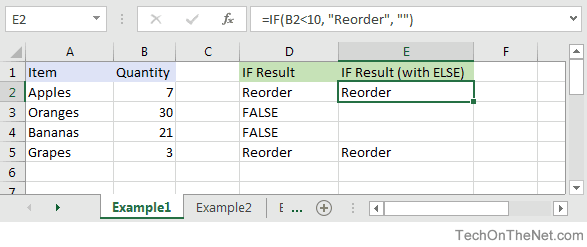
Based on the Excel spreadsheet above, the following IF examples would return:
=IF(B2<10, "Reorder", "")
Result: "Reorder"

=IF(A2="Apples", "Equal", "Not Equal")
Result: "Equal"

=IF(B3>=20, 12, 0)
Result: 12
Combining the IF function with Other Logical Functions
Quite often, you will need to specify more complex conditions when writing your formula in Excel. You can combine the IF function with other logical functions such as AND, OR, etc. Let’s explore this further.
AND function
The IF function can be combined with the AND function to allow you to test for multiple conditions. When using the AND function, all conditions within the AND function must be TRUE for the condition to be met. This comes in very handy in Excel formulas.
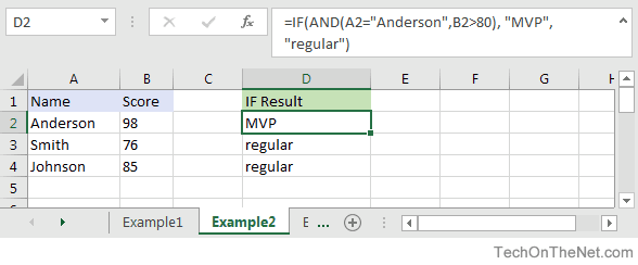
Based on the spreadsheet above, you can combine the IF function with the AND function as follows:
=IF(AND(A2="Anderson",B2>80), "MVP", "regular")
Result: "MVP"

=IF(AND(B2>=80,B2<=100), "Great Score", "Not Bad")
Result: "Great Score"

=IF(AND(B3>=80,B3<=100), "Great Score", "Not Bad")
Result: "Not Bad"

=IF(AND(A2="Anderson",A3="Smith",A4="Johnson"), 100, 50)
Result: 100

=IF(AND(A2="Anderson",A3="Smith",A4="Parker"), 100, 50)
Result: 50
In the examples above, all conditions within the AND function must be TRUE for the condition to be met.
OR function
The IF function can be combined with the OR function to allow you to test for multiple conditions. But in this case, only one or more of the conditions within the OR function needs to be TRUE for the condition to be met.
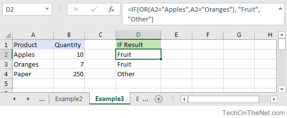
Based on the spreadsheet above, you can combine the IF function with the OR function as follows:
=IF(OR(A2="Apples",A2="Oranges"), "Fruit", "Other")
Result: "Fruit"

=IF(OR(A4="Apples",A4="Oranges"),"Fruit","Other")
Result: "Other"

=IF(OR(A4="Bananas",B4>=100), 999, "N/A")
Result: 999

=IF(OR(A2="Apples",A3="Apples",A4="Apples"), "Fruit", "Other")
Result: "Fruit"
In the examples above, only one of the conditions within the OR function must be TRUE for the condition to be met.
Let’s take a look at one more example that involves ranges of percentages.
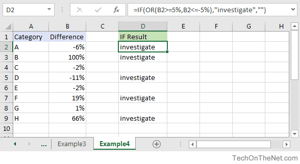
Based on the spreadsheet above, we would have the following formula in cell D2:
=IF(OR(B2>=5%,B2<=-5%),"investigate","")
Result: "investigate"
This IF function would return «investigate» if the value in cell B2 was either below -5% or above 5%. Since -6% is below -5%, it will return «investigate» as the result. We have copied this formula into cells D3 through D9 to show you the results that would be returned.
For example, in cell D3, we would have the following formula:
=IF(OR(B3>=5%,B3<=-5%),"investigate","")
Result: "investigate"
This formula would also return «investigate» but this time, it is because the value in cell B3 is greater than 5%.
Frequently Asked Questions
Question: In Microsoft Excel, I’d like to use the IF function to create the following logic:
if C11>=620, and C10=»F»or»S», and C4<=$1,000,000, and C4<=$500,000, and C7<=85%, and C8<=90%, and C12<=50, and C14<=2, and C15=»OO», and C16=»N», and C19<=48, and C21=»Y», then reference cell A148 on Sheet2. Otherwise, return an empty string.
Answer: The following formula would accomplish what you are trying to do:
=IF(AND(C11>=620, OR(C10="F",C10="S"), C4<=1000000, C4<=500000, C7<=0.85, C8<=0.9, C12<=50, C14<=2, C15="OO", C16="N", C19<=48, C21="Y"), Sheet2!A148, "")
Question: In Microsoft Excel, I’m trying to use the IF function to return 0 if cell A1 is either < 150,000 or > 250,000. Otherwise, it should return A1.
Answer: You can use the OR function to perform an OR condition in the IF function as follows:
=IF(OR(A1<150000,A1>250000),0,A1)
In this example, the formula will return 0 if cell A1 was either less than 150,000 or greater than 250,000. Otherwise, it will return the value in cell A1.
Question: In Microsoft Excel, I’m trying to use the IF function to return 25 if cell A1 > 100 and cell B1 < 200. Otherwise, it should return 0.
Answer: You can use the AND function to perform an AND condition in the IF function as follows:
=IF(AND(A1>100,B1<200),25,0)
In this example, the formula will return 25 if cell A1 is greater than 100 and cell B1 is less than 200. Otherwise, it will return 0.
Question: In Microsoft Excel, I need to write a formula that works this way:
IF (cell A1) is less than 20, then times it by 1,
IF it is greater than or equal to 20 but less than 50, then times it by 2
IF its is greater than or equal to 50 and less than 100, then times it by 3
And if it is great or equal to than 100, then times it by 4
Answer: You can write a nested IF statement to handle this. For example:
=IF(A1<20, A1*1, IF(A1<50, A1*2, IF(A1<100, A1*3, A1*4)))
Question: In Microsoft Excel, I need a formula in cell C5 that does the following:
IF A1+B1 <= 4, return $20
IF A1+B1 > 4 but <= 9, return $35
IF A1+B1 > 9 but <= 14, return $50
IF A1+B1 >= 15, return $75
Answer: In cell C5, you can write a nested IF statement that uses the AND function as follows:
=IF((A1+B1)<=4,20,IF(AND((A1+B1)>4,(A1+B1)<=9),35,IF(AND((A1+B1)>9,(A1+B1)<=14),50,75)))
Question: In Microsoft Excel, I need a formula that does the following:
IF the value in cell A1 is BLANK, then return «BLANK»
IF the value in cell A1 is TEXT, then return «TEXT»
IF the value in cell A1 is NUMERIC, then return «NUM»
Answer: You can write a nested IF statement that uses the ISBLANK function, the ISTEXT function, and the ISNUMBER function as follows:
=IF(ISBLANK(A1)=TRUE,"BLANK",IF(ISTEXT(A1)=TRUE,"TEXT",IF(ISNUMBER(A1)=TRUE,"NUM","")))
Question: In Microsoft Excel, I want to write a formula for the following logic:
IF R1<0.3 AND R2<0.3 AND R3<0.42 THEN «OK» OTHERWISE «NOT OK»
Answer: You can write an IF statement that uses the AND function as follows:
=IF(AND(R1<0.3,R2<0.3,R3<0.42),"OK","NOT OK")
Question: In Microsoft Excel, I need a formula for the following:
IF cell A1= PRADIP then value will be 100
IF cell A1= PRAVIN then value will be 200
IF cell A1= PARTHA then value will be 300
IF cell A1= PAVAN then value will be 400
Answer: You can write an IF statement as follows:
=IF(A1="PRADIP",100,IF(A1="PRAVIN",200,IF(A1="PARTHA",300,IF(A1="PAVAN",400,""))))
Question: In Microsoft Excel, I want to calculate following using an «if» formula:
if A1<100,000 then A1*.1% but minimum 25
and if A1>1,000,000 then A1*.01% but maximum 5000
Answer: You can write a nested IF statement that uses the MAX function and the MIN function as follows:
=IF(A1<100000,MAX(25,A1*0.1%),IF(A1>1000000,MIN(5000,A1*0.01%),""))
Question: In Microsoft Excel, I am trying to create an IF statement that will repopulate the data from a particular cell if the data from the formula in the current cell equals 0. Below is my attempt at creating an IF statement that would populate the data; however, I was unsuccessful.
=IF(IF(ISERROR(M24+((L24-S24)/AA24)),"0",M24+((L24-S24)/AA24)))=0,L24)
The initial part of the formula calculates the EAC (Estimate At completion = AC+(BAC-EV)/CPI); however if the current EV (Earned Value) is zero, the EAC will equal zero. IF the outcome is zero, I would like the BAC (Budget At Completion), currently recorded in another cell (L24), to be repopulated in the current cell as the EAC.
Answer: You can write an IF statement that uses the OR function and the ISERROR function as follows:
=IF(OR(S24=0,ISERROR(M24+((L24-S24)/AA24))),L24,M24+((L24-S24)/AA24))
Question: I have been looking at your Excel IF, AND and OR sections and found this very helpful, however I cannot find the right way to write a formula to express if C2 is either 1,2,3,4,5,6,7,8,9 and F2 is F and F3 is either D,F,B,L,R,C then give a value of 1 if not then 0. I have tried many formulas but just can’t get it right, can you help please?
Answer: You can write an IF statement that uses the AND function and the OR function as follows:
=IF(AND(C2>=1,C2<=9, F2="F",OR(F3="D",F3="F",F3="B",F3="L",F3="R",F3="C")),1,0)
Question:In Excel, I have a roadspeed of a car in m/s in cell A1 and a drop down menu of different units in C1 (which unclude mph and kmh). I have used the following IF function in B1 to convert the number to the unit selected from the dropdown box:
=IF(C1="mph","=A1*2.23693629",IF(C1="kmh","A1*3.6"))
However say if kmh was selected B1 literally just shows A1*3.6 and does not actually calculate it. Is there away to get it to calculate it instead of just showing the text message?
Answer: You are very close with your formula. Because you are performing mathematical operations (such as A1*2.23693629 and A1*3.6), you do not need to surround the mathematical formulas in quotes. Quotes are necessary when you are evaluating strings, not performing math.
Try the following:
=IF(C1="mph",A1*2.23693629,IF(C1="kmh",A1*3.6))
Question:For an IF statement in Excel, I want to combine text and a value.
For example, I want to put an equation for work hours and pay. IF I am paid more than I should be, I want it to read how many hours I owe my boss. But if I work more than I am paid for, I want it to read what my boss owes me (hours*Pay per Hour).
I tried the following:
=IF(A2<0,"I owe boss" abs(A2) "Hours","Boss owes me" abs(A2)*15 "dollars")
Is it possible or do I have to do it in 2 separate cells? (one for text and one for the value)
Answer: There are two ways that you can concatenate text and values. The first is by using the & character to concatenate:
=IF(A2<0,"I owe boss " & ABS(A2) & " Hours","Boss owes me " & ABS(A2)*15 & " dollars")
Or the second method is to use the CONCATENATE function:
=IF(A2<0,CONCATENATE("I owe boss ", ABS(A2)," Hours"), CONCATENATE("Boss owes me ", ABS(A2)*15, " dollars"))
Question:I have Excel 2000. IF cell A2 is greater than or equal to 0 then add to C1. IF cell B2 is greater than or equal to 0 then subtract from C1. IF both A2 and B2 are blank then equals C1. Can you help me with the IF function on this one?
Answer: You can write a nested IF statement that uses the AND function and the ISBLANK function as follows:
=IF(AND(ISBLANK(A2)=FALSE,A2>=0),C1+A2, IF(AND(ISBLANK(B2)=FALSE,B2>=0),C1-B2, IF(AND(ISBLANK(A2)=TRUE, ISBLANK(B2)=TRUE),C1,"")))
Question:How would I write this equation in Excel? IF D12<=0 then D12*L12, IF D12 is > 0 but <=600 then D12*F12, IF D12 is >600 then ((600*F12)+((D12-600)*E12))
Answer: You can write a nested IF statement as follows:
=IF(D12<=0,D12*L12,IF(D12>600,((600*F12)+((D12-600)*E12)),D12*F12))
Question:In Excel, I have this formula currently:
=IF(OR(A1>=40, B1>=40, C1>=40), "20", (A1+B1+C1)-20)
If one of my salesman does sale for $40-$49, then his commission is $20; however if his/her sale is less (for example $35) then the commission is that amount minus $20 ($35-$20=$15). I have 3 columns that are needed based on the type of sale. Only one column per row will be needed. The problem is that, when left blank, the total in the formula cell is -20. I need help setting up this formula so that when the 3 columns are left blank, the cell with the formula is left blank as well.
Answer: Using the AND function and the ISBLANK function, you can write your IF statement as follows:
=IF(AND(ISBLANK(A1),ISBLANK(B1),ISBLANK(C1)),"",IF(OR(A1>40, B1>40, C1>40), "20", (A1+B1+C1)-20))
In this formula, we are using the ISBLANK function to check if all 3 cells A1, B1, and C1 are blank, and if they are return a blank value («»). Then the rest is the formula that you originally wrote.
Question:In Excel, I need to create a simple booking and and out system, that shows a date out and a date back
«A1» = allows person to input date booked out
«A2» =allows person to input date booked back in
«A3″= shows status of product, eg, booked out, overdue return etc.
I can automate A3 with the following IF function:
=IF(ISBLANK(A2),"booked out","returned")
But what I cant get to work is if the product is out for 10 days or more, I would like the cell to say «send email»
Can you assist?
Answer: Using the TODAY function and adding an additional IF function, you can write your formula as follows:
=IF(ISBLANK(A2),IF(TODAY()-A1>10,"send email","booked out"),"returned")
Question:Using Microsoft Excel, I need a formula in cell U2 that does the following:
IF the date in E2<=12/31/2010, return T2*0.75
IF the date in E2>12/31/2010 but <=12/31/2011, return T2*0.5
IF the date in E2>12/31/2011, return T2*0
I tried using the following formula, but it gives me «#VALUE!»
=IF(E2<=DATE(2010,12,31),T2*0.75), IF(AND(E2>DATE(2010,12,31),E2<=DATE(2011,12,31)),T2*0.5,T2*0)
Can someone please help? Thanks.
Answer: You were very close…you just need to adjust your parentheses as follows:
=IF(E2<=DATE(2010,12,31),T2*0.75, IF(AND(E2>DATE(2010,12,31),E2<=DATE(2011,12,31)),T2*0.5,T2*0))
Question:In Excel, I would like to add 60 days if grade is ‘A’, 45 days if grade is ‘B’ and 30 days if grade is ‘C’. It would roughly look something like this, but I’m struggling with commas, brackets, etc.
(IF C5=A)=DATE(YEAR(B5)+0,MONTH(B5)+0,DAY(B5)+60),
(IF C5=B)=DATE(YEAR(B5)+0,MONTH(B5)+0,DAY(B5)+45),
(IF C5=C)=DATE(YEAR(B5)+0,MONTH(B5)+0,DAY(B5)+30)
Answer:You should be able to achieve your date calculations with the following formula:
=IF(C5="A",B5+60,IF(C5="B",B5+45,IF(C5="C",B5+30)))
Question:In Excel, I am trying to write a function and can’t seem to figure it out. Could you help?
IF D3 is < 31, then 1.51
IF D3 is between 31-90, then 3.40
IF D3 is between 91-120, then 4.60
IF D3 is > 121, then 5.44
Answer:You can write your formula as follows:
=IF(D3>121,5.44,IF(D3>=91,4.6,IF(D3>=31,3.4,1.51)))
Question:I would like ask a question regarding the IF statement. How would I write in Excel this problem?
I have to check if cell A1 is empty and if not, check if the value is less than equal to 5. Then multiply the amount entered in cell A1 by .60. The answer will be displayed on Cell A2.
Answer:You can write your formula in cell A2 using the IF function and ISBLANK function as follows:
=IF(AND(ISBLANK(A1)=FALSE,A1<=5),A1*0.6,"")
Question:In Excel, I’m trying to nest an OR command and I can’t find the proper way to write it. I want the spreadsheet to do the following:
If D6 equals «HOUSE» and C6 equals either «MOUSE» or «CAT», I want to return the value in cell B6. Otherwise, the formula should return the value «BLANK».
I tried the following:
=IF((D6="HOUSE")*(C6="MOUSE")*OR(C6="CAT"));B6;"BLANK")
If I only ask for HOUSE and MOUSE or HOUSE and CAT, it works, but as soon as I ask for MOUSE OR CAT, it doesn’t work.
Answer:You can write your formula using the AND function and OR function as follows:
=IF(AND(D6="HOUSE",OR(C6="MOUSE",C6="CAT")),B6,"BLANK")
This will return the value in B6 if D6 equals «HOUSE» and C6 equals either «MOUSE» or «CAT». If those conditions are not met, the formula will return the text value of «BLANK».
Question:In Microsoft Excel, I’m trying to write the following formula:
If cell A1 equals «jaipur», «udaipur» or «jodhpur», then cell A2 should display «rajasthan»
If cell A1 equals «bangalore», «mysore» or «belgum», then cell A2 should display «karnataka»
Please help.
Answer:You can write your formula using the OR function as follows:
=IF(OR(A1="jaipur",A1="udaipur",A1="jodhpur"),"rajasthan", IF(OR(A1="bangalore",A1="mysore",A1="belgum"),"karnataka"))
This will return «rajasthan» if A1 equals either «jaipur», «udaipur» or «jodhpur» and it will return «karnataka» if A1 equals either «bangalore», «mysore» or «belgum».
Question:In Microsoft Excel I’m trying to achieve the following with IF function:
If a value in any cell in column F is «food» then add the value of its corresponding cell in column G (eg a corresponding cell for F3 is G3). The IF function is performed in another cell altogether. I can do it for a single pair of cells but I don’t know how to do it for an entire column. Could you help?
At the moment, I’ve got this:
=IF(F3="food"; G3; 0)
Answer:This formula can be created using the SUMIF formula instead of using the IF function:
=SUMIF(F1:F10,"=food",G1:G10)
This will evaluate the first 10 rows of data in your spreadsheet. You may need to adjust the ranges accordingly.
I notice that you separate your parameters with semi-colons, so you might need to replace the commas in the formula above with semi-colons.
Question:I’m looking for an Exel formula that says:
If F3 is «H» and E3 is «H», return 1
If F3 is «A» and E3 is «A», return 2
If F3 is «d» and E3 is «d», return 3
Appreciate if you can help.
Answer:This Excel formula can be created using the AND formula in combination with the IF function:
=IF(AND(F3="H",E3="H"),1,IF(AND(F3="A",E3="A"),2,IF(AND(F3="d",E3="d"),3,"")))
We’ve defaulted the formula to return a blank if none of the conditions above are met.
Question:I am trying to get Excel to check different boxes and check if there is text/numbers listed in the cells and then spit out «Complete» if all 5 Boxes have text/Numbers or «Not Complete» if one or more is empty. This is what I have so far and it doesn’t work.
=IF(OR(ISBLANK(J2),ISBLANK(M2),ISBLANK(R2),ISBLANK (AA2),ISBLANK (AB2)),"Not Complete","")
Answer:First, you are correct in using the ISBLANK function, however, you have a space between ISBLANK and (AA2), as well as ISBLANK and (AB2). This might seem insignificant, but Excel can be very picky and will return a #NAME? error. So first you need to eliminate those spaces.
Next, you need to change the ELSE condition of your IF function to return «Complete».
You should be able to modify your formula as follows:
=IF(OR(ISBLANK(J2),ISBLANK(M2),ISBLANK(R2),ISBLANK(AA2),ISBLANK(AB2)), "Not Complete", "Complete")
Now if any of the cell J2, M2, R2, AA2, or AB2 are blank, the formula will return «Not Complete». If all 5 cells have a value, the formula will return «Complete».
Question:I’m very new to the Excel world, and I’m trying to figure out how to set up the proper formula for an If/then cell.
What I’m trying for is:
If B2’s value is 1 to 5, then multiply E2 by .77
If B2’s value is 6 to 10, then multiply E2 by .735
If B2’s value is 11 to 19, then multiply E2 by .7
If B2’s value is 20 to 29, then multiply E2 by .675
If B2’s value is 30 to 39, then multiply E2 by .65
I’ve tried a few different things thinking I was on the right track based on the IF, and AND function tutorials here, but I can’t seem to get it right.
Answer:To write your IF formula, you need to nest multiple IF functions together in combination with the AND function.
The following formula should work for what you are trying to do:
=IF(AND(B2>=1, B2<=5), E2*0.77, IF(AND(B2>=6, B2<=10), E2*0.735, IF(AND(B2>=11, B2<=19), E2*0.7, IF(AND(B2>=20, B2<=29), E2*0.675, IF(AND(B2>=30, B2<=39), E2*0.65,"")))))
As one final component of your formula, you need to decide what to do when none of the conditions are met. In this example, we have returned «» when the value in B2 does not meet any of the IF conditions above.
Question:Here is the Excel formula that has me between a rock and a hard place.
If E45 <= 50, return 44.55
If E45 > 50 and E45 < 100, return 42
If E45 >=200, return 39.6
Again thank you very much.
Answer:You should be able to write this Excel formula using a combination of the IF function and the AND function.
The following formula should work:
=IF(E45<=50, 44.55, IF(AND(E45>50, E45<100), 42, IF(E45>=200, 39.6, "")))
Please note that if none of the conditions are met, the Excel formula will return «» as the result.
Question:I have a nesting OR function problem:
My nonworking formula is:
=IF(C9=1,K9/J7,IF(C9=2,K9/J7,IF(C9=3,K9/L7,IF(C9=4,0,K9/N7))))
In Cell C9, I can have an input of 1, 2, 3, 4 or 0. The problem is on how to write the «or» condition when a «4 or 0» exists in Column C. If the «4 or 0» conditions exists in Column C I want Column K divided by Column N and the answer to be placed in Column M and associated row
Answer:You should be able to use the OR function within your IF function to test for C9=4 OR C9=0 as follows:
=IF(C9=1,K9/J7,IF(C9=2,K9/J7,IF(C9=3,K9/L7,IF(OR(C9=4,C9=0),K9/N7))))
This formula will return K9/N7 if cell C9 is either 4 or 0.
Question:In Excel, I am trying to create a formula that will show the following:
If column B = Ross and column C = 8 then in cell AB of that row I want it to show 2013, If column B = Block and column C = 9 then in cell AB of that row I want it to show 2012.
Answer:You can create your Excel formula using nested IF functions with the AND function.
=IF(AND(B1="Ross",C1=8),2013,IF(AND(B1="Block",C1=9),2012,""))
This formula will return 2013 as a numeric value if B1 is «Ross» and C1 is 8, or 2012 as a numeric value if B1 is «Block» and C1 is 9. Otherwise, it will return blank, as denoted by «».
Question:In Excel, I really have a problem looking for the right formula to express the following:
If B1=0, C1 is equal to A1/2
If B1=1, C1 is equal to A1/2 times 20%
If D1=1, C1 is equal to A1/2-5
I’ve been trying to look for any same expressions in your site. Please help me fix this.
Answer:In cell C1, you can use the following Excel formula with 3 nested IF functions:
=IF(B1=0,A1/2, IF(B1=1,(A1/2)*0.2, IF(D1=1,(A1/2)-5,"")))
Please note that if none of the conditions are met, the Excel formula will return «» as the result.
Question:In Excel, I need the answer for an IF THEN statement which compares column A and B and has an «OR condition» for column C. My problem is I want column D to return yes if A1 and B1 are >=3 or C1 is >=1.
Answer:You can create your Excel IF formula as follows:
=IF(OR(AND(A1>=3,B1>=3),C1>=1),"yes","")
Please note that if none of the conditions are met, the Excel formula will return «» as the result.
Question:In Excel, what have I done wrong with this formula?
=IF(OR(ISBLANK(C9),ISBLANK(B9)),"",IF(ISBLANK(C9),D9-TODAY(), "Reactivated"))
I want to make an event that if B9 and C9 is empty, the value would be empty. If only C9 is empty, then the output would be the remaining days left between the two dates, and if the two cells are not empty, the output should be the string ‘Reactivated’.
The problem with this code is that IF(ISBLANK(C9),D9-TODAY() is not working.
Answer:First of all, you might want to replace your OR function with the AND function, so that your Excel IF formula looks like this:
=IF(AND(ISBLANK(C9),ISBLANK(B9)),"",IF(ISBLANK(C9),D9-TODAY(),"Reactivated"))
Next, make sure that you don’t have any abnormal formatting in the cell that contains the results. To be safe, right click on the cell that contains the formula and choose Format Cells from the popup menu. When the Format Cells window appears, select the Number tab. Choose General as the format and click on the OK button.
Question:I was wondering if you could tell me what I am doing wrong.
Here are the instructions:
A customer is eligible for a discount if the customer’s 2016 sales greater than or equal to 100000 OR if the customers First Order was placed in 2016.
If the customer qualifies for a discount, return a value of Y
If the customer does not qualify for a discount, return a value of N.
Here is the formula I’ve entered:
=IF(OR([2014 Sales]=0,[2015 Sales]=0,[2016 Sales]>=100000),"Y","N")
I only have 2 cells wrong. Can you help me please? I am very lost and confused.
Answer:You are very close with your IF formula, however, it looks like you need to add the AND function to your formula as follows:
=IF(OR([2016 Sales]>=100000,AND([2014 Sales]=0,[2015 Sales]=0),C8>=100000),"Y","N")
This formula should return Y if 2016 sales are greater than or equal to 100000, or if both 2014 sales and 2015 sales are 0. Otherwise, the formula will return N. You will also notice that we switched the order of your conditions in the formula so that it is easier to understand the formula based on your instructions above.
Question:Could you please help me? I need to use «OR» on my formula but I can’t get it to work. This is what I’ve tried:
=IF(C6>=0<=150,150000,IF(C6>=151<=160,158400))
Here is what I need the formula to do:
IF C6 IS >=0 OR <=150 THEN ASSIGN $150000
IF C6 IS >=151 OR <=160 THEN ASSIGN $158400
Answer:You should be able to use the AND function within your IF function as follows:
=IF(AND(ISBLANK(C6)=FALSE,C6>=0,C6<=150),150000,IF(AND(C6>=151,C6<=160),158400,""))
Notice that we first use the ISBLANK function to test C6 to make sure that it is not blank. This is because if C6 if blank, it will evalulate to greater than 0 and thus return 150000. To avoid this, we include ISBLANK(C6)=FALSE as one of the conditions in addition to C6>=0 and C6<=150. That way, you won’t return any false results if C6 is blank.
Question:I am having a problem with a formula, I want it to be IF E5=N then do the first formula, else do the second formula. Excel recognizes the =IF(logical_test,value_if_TRUE,value_if_FALSE) but doesn’t like the formula below:
=IF(e5="N",((AND(AH5-AG5<456, AH5-S5<822)), "Compliant", "not Compliant"),((AH5-S5<822), "Compliant", "not Compliant"))
Any help would be greatly appreciated.
Answer:To have the first formula executed when E5=N and then second formula executed when E5<>N, you will need to nest 2 additional IF functions within the main IF function as follows:
=IF(E5="N", IF((AND(AH5-AG5<456, AH5-S5<822)), "Compliant", "not Compliant"), IF((AH5-S5<822), "Compliant", "not Compliant"))
If E5=»N», the first nested IF function will be executed:
IF((AND(AH5-AG5<456, AH5-S5<822)), "Compliant", "not Compliant")
Otherwise,the second nested IF function will be executed:
IF((AH5-S5<822), "Compliant", "not Compliant"))
Question:I need to write a formula based on the following logic:
There is a maximum discount allowed of £1000 if the capital sum is less that £43000 and a lower discount of £500 if the capital sum is above £43000. So the formula should return either £500 or £1000 in the cell but the £43000 is made up of two numbers, say for e.g. £42750+350 and if the second number is less than the allowed discount, the actual lower value is returned — in this case the £500 or £1000 becomes £350. Or as another e.g. £42000+750 returns £750.
So on my spreadsheet, in this second e.g. I would have A1= £42000, A2=750, A3=A1+A2, A4=the formula with the changing discount, in this case £750.
How can I write this formula?
Answer:In cell A4, you can calculate the correct discount using the IF function and the MIN function as follows:
=IF(A3<43000, MIN(A2,1000), MIN(A2,500))
If A3 is less than 43000, the formula will return the lower value of A2 and 1000. Otherwise, it will return the lower value of A2 and 500.
Question: I have a list of sizes in column A with sizes 100, 200, 300, 400, 500, 600. Then I have another column B, with sizes of my products, and it is random, for example, 318, 445, 527. What I’m trying to create is for a value of 318 in column B, I need to return 400 for that product. If the value in column B is 445, then I should return 500 and so on, as long sizes in column A must be BIGGER to the NEAREST size to column B.
Any idea how to create this function?
Answer:If your sizes are in increments of 100, you can create this function by taking the value in column B, dividing by 100, rounding up to the nearest integer, and then multiplying by 100.
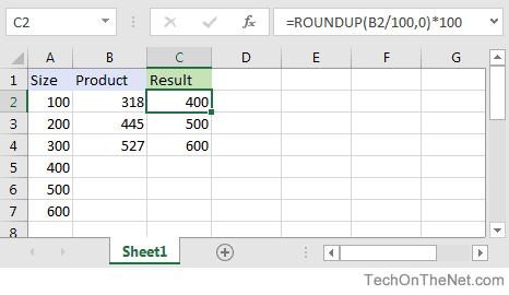
For example in cell C2, you can use the IF function and the ROUNDUP function as follows:
=ROUNDUP(B2/100,0)*100
This will return the correct value of 400 for a value of 318 in cell B2. Just copy this formula to cell C3, C4 and so on.
This is a step-by-step guide on how to use IF function in Excel. It shows you how to create a formula using the IF function, it includes several IF formula examples, an introduction on how to use nested IF formulas, and the exercise file I used when creating this tutorial.
The Excel IF function performs a logical test and returns one value when the condition is TRUE and another when the condition is FALSE.
How do you write an if-then formula in Excel? Well, the syntax for IF statements is the same in all Excel versions. This means that you can use any of the examples shown in this article in Excel for Microsoft 365 or Excel 2021, 2019, 2016, 2013, 2010, 2007, and 2003.
How to use IF function in Excel:
- Select the cell where you want to insert the IF formula. Using your mouse or keyboard, navigate to the cell where you want to insert your formula.
- Type =IF(
- Insert the condition that you want to check, followed by a comma (,). The first argument of the IF function is the logical_test. This is the condition that you want to validate. For example C6 > 70.
- Insert the value to display when the condition is TRUE, followed by a comma (,). The second argument of the IF function is value_if_true. Here, you can insert a nested formula or a simple message such as “YES”.
- Insert the value to display when the condition is FALSE. The last argument of the IF function is value_if_false. Just like the previous step, you can insert a nested formula or display a message such as “NO”. This can also be set as an empty string (“”), which will display a cell that looks blank.
- Type ) to close the function and press ENTER
The following video shows you exactly how to apply the six steps described above and create your first IF formula.
The syntax that shows how to create an IF function in Excel is explained below:=IF(logical_test, [value_if_true], [value_if_false])
IF is a logical function and implies setting 3 arguments:
logical_test – The logical condition that you want to test. This will return either a TRUE or a FALSE value.
value_if_true – [optional] The value or formula which will be used when logical_test is TRUE.
value_if_false – [optional] The value or formula which will be used when logical_test is FALSE.
Please remember that while both value_if_true and value_if_false are optional, at least one of them needs to be supplied. Otherwise, your IF formula will simply return 0 (zero).
Where is the IF function in Excel? Since this is a logical function, you can find the IF function in the Formulas tab, Function Library section, under Logical.
Logical operators for IF function
The IF function is one of the most used Excel functions, and it allows you to return different values when the logical condition supplied is TRUE or FALSE. An Excel if-then formula can use the following logical operators:
| Logical operators | Definition | Example |
| = | equal to | A1=B1 |
| <> | not equal to | A1<>B1 |
| > | greater than | A1>B1 |
| >= | greater than or equal to | A1>=B1 |
| < | lower than | A1<B1 |
| <= | lower than or equal to | A1<=B1 |
The IF function doesn’t support wildcards.
Your first IF formula
The IF function runs a logical test and returns different values depending on whether the result is TRUE or FALSE. The result from IF can be a value, a cell reference, or even another formula.
Now let’s move on to some examples.
We’ll be evaluating exam grades. If the student obtained a score higher than or equal to 70, then we will return the message “Pass.” If the grade is lower than 70, then we will display “Fail.”
In this example, I have inserted the following formula in cell F9:=IF(E9>=70, "Pass", "Fail")
The 3 arguments for this IF formula are:
logical_test: E9>=70
value_if_true: Pass is returned if E9>=70.
value_if_false: Fail is returned if E9<70.

Please note that when you want to use text in your IF formulas (like a word or sentence), you need to wrap the text in quotes (e.g. “Fail”). The only exception is while using TRUE or FALSE, which are built-in functionalities that Excel recognizes automatically.
How to use the IF function in Excel with another function or formula
The beauty of the IF function is that it allows us to build complex financial models with lots of interdependencies. This includes using different formulas based on conditional logic.
In our next example, we will use the IF function to calculate a payment fee based on the value of the order. If the order value is higher than or equal to $1000, then it should calculate a payment fee of 1.00%. However, if the total order value is lower than $1000, then it should use 1.50%.
The formula in cell F31 is:=IF(E31>=1000, E31*1%, E31*1.5%)

Now let’s look at an IF formula that is dependent on user input. If we select free shipping for the order, then the shipping fee will be set to zero. Otherwise, it will be calculated as 3% of the order value.
This is something really easy to achieve, but it will open up so many opportunities for you to use the IF function in the future.

How to use nested IF statements in Excel
Nesting more IF functions allows you to perform multiple comparisons and create more complex formulas. However, you can only nest up to 64 IF functions in Excel. If you ever reach this limit (I never did), I can guarantee that there is a better and more elegant solution using functions like VLOOKUP, SUMIF, or COUNTIFS.
In the next example, I wrote a formula with several nested IF functions to assign a grade to a list of students based on their test results.
=IF(E71<60, "F", IF(E71<70, "D", IF(E71<80, "C", IF(E71<90, "B", "A"))))
The order of the conditions is important. When the conditions overlap, Excel will retrieve the [value_if_true] argument from the first IF statement that returns TRUE. This is why the conditions from the formula above need to be inserted in the same order for the formula to work properly.

Note: If you are running Office 365, then you can also look at the new IFS function. This function runs multiple tests and returns the value corresponding to the first TRUE result. It’s a very useful alternative to nested IF formulas and makes your formulas much easier to understand by others. You can read more about IFS on Microsoft’s website.
How to use IF formula with OR function in Excel
OR allows you to supply alternative conditions to an IF statement. This opens up opportunities to create complex scenarios where certain behavior is triggered by multiple possible conditions.
Let’s look at an IF formula that calculates a 2.00% shipping fee when the total order value is higher than $1000 or when there are more than 5 items in the order.
The IF OR statement I’ve used in cell H106 is:=IF(OR(G106>1000, F106>5), G106*2%, 0)

The OR function evaluates if G106>1000 or if F106>5 and the formula returns TRUE when either or both conditions are fulfilled.
How to use IF formula with AND function in Excel
AND allows you to supply multiple criteria to an IF statement. Basically, the IF function returns TRUE if, and only if, all the conditions are met.
Working with our previous example, let’s apply the shipping fee only when the total order value is higher than $1000 and the order contains more than 5 items.
The IF AND statement I’ve used in cell H106 is:=IF(AND(G128>1000, F128>5), G128*2%, 0)

The AND function evaluates if G106>1000 and if F106>5 and returns TRUE when both conditions are fulfilled.
How to use IF function with VLOOKUP in Excel
VLOOKUP can be nested inside an IF formula to retrieve data when a condition is TRUE or FALSE. In the next example, I will show you how to calculate shipping fees based on a different table that contains the thresholds and percentages to be applied depending on the order value.
The formula I’ve used in cell F152:=IF(G152="No", VLOOKUP(E152, $J$146:$K$152, 2, TRUE)*E152, 0)

The formula uses the following arguments:
logical_test: G152="No"
value_if_true: VLOOKUP(E152, $J$146:$K$152, 2, TRUE)*E152 is used to retrieve the corresponding shipping fee percentage when G152=”No”
value_if_false: 0 is returned if G152 is anything else than “No.” In our case, the alternative is selecting “Yes” from the drop-down list.
Note: One thing to remember is that I’ve used a VLOOKUP formula with an approximate match argument. This means that your data must be sorted in ascending order by lookup value (in our case, the Order amount).
In case you need additional help, please also read this article that explains step-by-step how to use VLOOKUP function in Excel.
What to do next?
IF is a versatile function that can be used in a wide range of scenarios. I use it daily, and I can’t imagine a world where Excel would lack this functionality.
Practice writing formulas using the IF function, and your spreadsheets will definitely get better and more complex. For example, why not look at another example using an IF function with 3 conditions? It will show you more examples of how to insert an if formula in Excel using nested IF statements and multiple conditions.
Let me know if you have questions on how to use IF function in Excel or if you need advice on how to nest multiple IF statements in your Excel project by leaving a comment below.