
Excel for Microsoft 365 Excel for Microsoft 365 for Mac Excel for the web Excel 2021 Excel 2021 for Mac Excel 2019 Excel 2019 for Mac Excel 2016 Excel 2016 for Mac Excel 2013 Excel 2010 Excel 2007 Excel for Mac 2011 Excel Starter 2010 More…Less
This article describes the formula syntax and usage of the RATE function in Microsoft Excel.
Description
Returns the interest rate per period of an annuity. RATE is calculated by iteration and can have zero or more solutions. If the successive results of RATE do not converge to within 0.0000001 after 20 iterations, RATE returns the #NUM! error value.
Syntax
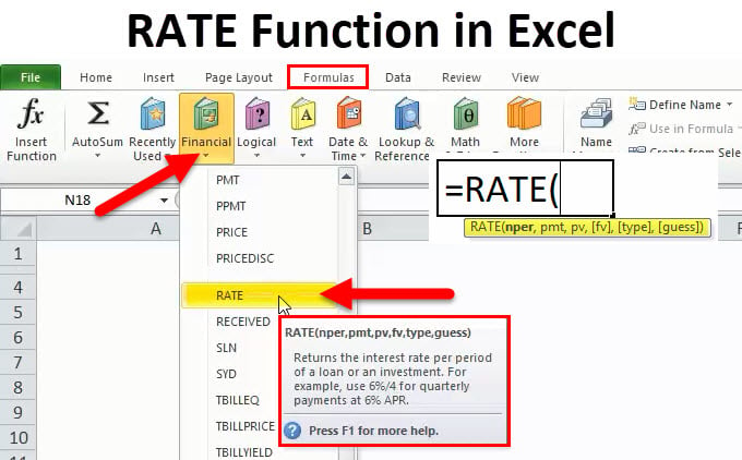
RATE(nper, pmt, pv, [fv], [type], [guess])
Note: For a complete description of the arguments nper, pmt, pv, fv, and type, see PV.
The RATE function syntax has the following arguments:
-
Nper Required. The total number of payment periods in an annuity.
-
Pmt Required. The payment made each period and cannot change over the life of the annuity. Typically, pmt includes principal and interest but no other fees or taxes. If pmt is omitted, you must include the fv argument.
-
Pv Required. The present value — the total amount that a series of future payments is worth now.
-
Fv Optional. The future value, or a cash balance you want to attain after the last payment is made. If fv is omitted, it is assumed to be 0 (the future value of a loan, for example, is 0). If fv is omitted, you must include the pmt argument.
-
Type Optional. The number 0 or 1 and indicates when payments are due.
|
Set type equal to |
If payments are due |
|
0 or omitted |
At the end of the period |
|
1 |
At the beginning of the period |
-
Guess Optional. Your guess for what the rate will be.
-
If you omit guess, it is assumed to be 10 percent.
-
If RATE does not converge, try different values for guess. RATE usually converges if guess is between 0 and 1.
-
Remarks
Make sure that you are consistent about the units you use for specifying guess and nper. If you make monthly payments on a four-year loan at 12 percent annual interest, use 12%/12 for guess and 4*12 for nper. If you make annual payments on the same loan, use 12% for guess and 4 for nper.
Example
Copy the example data in the following table, and paste it in cell A1 of a new Excel worksheet. For formulas to show results, select them, press F2, and then press Enter. If you need to, you can adjust the column widths to see all the data.
|
Data |
Description |
|
|
4 |
Years of the loan |
|
|
-200 |
Monthly payment |
|
|
8000 |
Amount of the loan |
|
|
Formula |
Description |
Result |
|
=RATE(A2*12, A3, A4) |
Monthly rate of the loan with the terms entered as arguments in A2:A4. |
1% |
|
=RATE(A2*12, A3, A4)*12 |
Annual rate of the loan with the same terms. |
9.24% |
Need more help?
Want more options?
Explore subscription benefits, browse training courses, learn how to secure your device, and more.
Communities help you ask and answer questions, give feedback, and hear from experts with rich knowledge.
The RATE function in Excel is used to calculate the rate levied on a period of a loan. It is a built-in function in Excel. It takes the number of payment periods, pmt, present value, and future value as an input. The input provided to this formula is in integers, and the output is in percentages.
For example, suppose we have a dataset of the 5-year loan of $25,000 in cell B1 with monthly payments of $1000 in cell B2 has 60 periods in cell B3. We need to find the interest rate on the student loan. In such a scenario, we can use the RATE function in Excel:
=RATE(B3,B2,-B1)*12
=4.1%.
Table of contents
- RATE Excel Function
- RATE Formula in Excel
- Explanation
- How to Use RATE Function in Excel?
- Example #1
- Example #2
- Example #3
- Example #4
- Things to Remember
- Recommended Articles
RATE Formula in Excel

Explanation
Compulsory Parameter:
- Nper: Nper is the total number of the period for the loan/investment amount to be paid. For example, considering the 5 years terms means 5*12=60.
- Pmt: The fixed amount paid per period cannot be changed during the annuity’s life.
- Pv: Pv is the total loan amount or present value.
Optional Parameter:
- [Fv]: It is also called the future value and is optional in the RATE function in Excel. And if not passed in this function, it will be considered zero.
- [Type]: It can be omitted from the RATE function in Excel and used as 1 if payments are due at the beginning of the period and considered as 0 in case the payments are due at the end of the period.
- [Guess]: It is also an optional parameter; if omitted, it is assumed as 10%.
How to Use the RATE Function in Excel?
The RATE function in Excel is very simple and easy to use and can be used as a worksheet function and VBA function. Therefore, this function is used as a worksheet function.
You can download this Rate Function Excel Template here – Rate Function Excel Template
Example #1
Suppose the investment amount is 25,000, and the period is 5 years. Here the number of payments nperNPER, commonly known as the number of payment periods for a loan, is a financial term and an inbuilt financial function in Excel that can be used to calculate NPER for any loan. This formula takes rate, payment made, present value and future value as input from a user.read more will be =5*12=60 payments in total, and we have considered 500 as a fixed monthly payment and then calculated the interest rate using the RATE function in Excel.

Output will be: =RATE (C5, C4,-C3)*12 = 7.4%
Example #2
Let us consider another example wherein the interest rate per payment period on a 5,000 investment amount where monthly payments of 250 are made for 2 years so period will be=12*2=24. Here we have considered that all payments are made at the beginning of the period, so the type will be 1.
Calculation of interest rate are as follows:
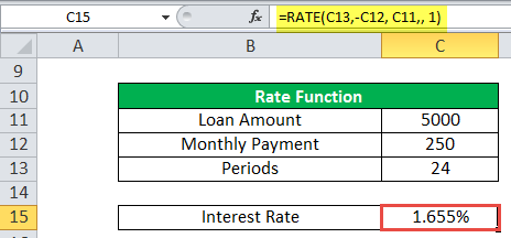
=RATE(C13,-C12, C11,, 1) output will be: 1.655%
Example #3
Let us take another example for weekly payment. This next example returns the interest rate on a loan amount of 8,000 where weekly payments of 700 are made for 4 years. Here, we have considered that all payments are made at the end of the period so that type will be 0 here.

The output will be: =RATE(C20,-C19, C18,, 0) = 8.750%.
Example #4
In the final example, we have considered that the loan amount will be 8,000, and annual payments of 950 are made for 10 years. Here, we assume that all the payments are made at the end of the period, then the type will be 0.
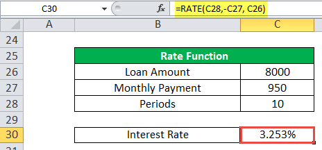
The output will be: =RATE(C28,-C27, C26) =3.253%
RATE in Excel is used as a VBA functionVBA functions serve the primary purpose to carry out specific calculations and to return a value. Therefore, in VBA, we use syntax to specify the parameters and data type while defining the function. Such functions are called user-defined functions.read more.
Dim Rate_value As Double
Rate_value = Rate(10*1, -950, 800)
Msgbox Rate_value
And output will be 0.3253
Things to Remember
Below are the few error details that can come in RATE in Excel if wrong arguments are passed in the RATE function in Excel.
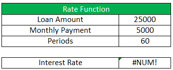
- Error handling #NUM!: If the interest RATE does not converge to 0.0000001 after 20 iterations, then the RATE excel function returns the #NUM! Error value.
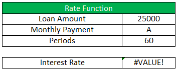
- Error handling #VALUE!: The RATE Excel function through a #VALUE! Error when any non-numeric value has been passed in the RATE formula in the Excel argument.
- We must convert the number of periods to month or quarter per your requirement.
- If the output of this function seems like 0, then there is no decimal value, then we must format the cell value to percentage format.
Recommended Articles
This article is a guide to Rate Function in Excel. Here, we discuss the RATE formula in Excel and how to use the RATE function, along with Excel examples and downloadable Excel templates. You may also look at these useful functions in Excel: –
- Negative Interest Rate MeaningWhen the interest rate falls below 0 percent, we have a negative interest scenario. This implies that banks will charge you interest for keeping your money with them. It is more common during periods of extreme deflation.read more
- Excel Record MacrosRecording macros is a method whereby excel stores the tasks performed by the user. Every time a macro is run, these exact actions are performed automatically. Macros are created in either the View tab (under the “macros” drop-down) or the Developer tab of Excel.
read more - MODE Excel Function
- MONTH Excel FunctionThe Month Function is a date function that determines the month for a given date in date format. It takes an argument in a date format and displays the result in integer format.read more
- Insert (Embed) an Object in ExcelIn Microsoft Excel, the “Object Insert” option allows a user to insert an external object into a worksheet. Embedding generally means inserting an object from another software (Word, PDF, etc.) into an Excel worksheet.read more
Purpose
Get the interest rate per period of an annuity
Return value
The interest rate per period
Usage notes
The RATE function returns the interest rate per period of an annuity. You can use RATE to calculate the periodic interest rate, then multiply as required to derive the annual interest rate. The RATE function calculates by iteration. If the results of RATE do not converge within 20 iterations, RATE returns the #NUM! error value.
The RATE function takes six separate arguments, three of which are required as explained below.
nper (required) — The total number of payment periods in the annuity. For example, a 5-year car loan with monthly payments has 60 periods. You can enter nper as 5*12 to show how the number was determined.
pmt (required) — The payment made each period. This number cannot change over the life of the annuity. In annuity functions, cash paid out is represented by a negative number. Note: If pmt is not provided, the optional fv argument must be supplied.
pv (optional) — The present value. This is the cash balance required after all payments have been made.
fv (optional) — The future value, or a cash balance required after the last payment is made. When fv is omitted, it defaults to zero (0) and pmt must be provided.
type (optional) — type is a boolean that controls when when payments are due. Use 0 for payments due at the end of the period (regular annuities) and 1 for payments due at the end of the period (annuities due). Type defaults to 0 (end of period).
guess (optional) — guess is a seed value to use for iteration. When omitted, guess defaults to 10%. Ordinarily, you can safely omit guess. If RATE does not converge, RATE will return a #NUM! error. Try different values for guess between 0 and 1.
Example
To calculate the annual interest rate for a $5000 loan with payments of $93.22 per month over 5 years, you can use RATE in a formula like this:
=RATE(60,-93.22,5000)*12 // returns 4.5%
In the example shown, the formula in C10 is:
=RATE(C7,-C6,C5)*C8 // returns 4.5%
Notice the value for pmt from C6 is entered as a negative value.
Notes
You must use consistent values for for guess and nper. If you make monthly payments on a five-year loan at 10 percent annual interest, use 10%/12 for guess and 5*12 for nper. If you make annual payments on the same loan, use 10% for guess and 5 for nper.
RATE Function (Table of Contents)
- Introduction to RATE Function in Excel
- RATE Formula in Excel
- How to Use RATE Function?
Introduction to RATE Function in Excel
Let’s assume an example. Ram wants to take a loan/borrow some amount of money or wants to invest some money from a financial company XYZ. The company needs to do some financial calculations like the customer has to pay something to the financial company against loan amount or how much customer needs to invest so that after some time he/she can get this much amount of money.
In these scenarios, Excel has the most important function, “RATE”, which is part of a financial function.
What is the RATE Function?
A function that is used to calculate the interest rate for paying the specified amount of a loan or to get the specified amount of an investment after some period of time is called the RATE function.
RATE Formula in Excel
Below is the RATE Formula:
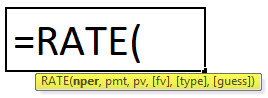
RATE function uses below arguments
Nper: The total no. of periods for the loan or an investment.
Pmt: The payment made each period, and this is a fixed amount during the loan or investment.
Pv: The current (Present) value of a loan/an investment.
[Fv]: That’s the optional argument. This specifies the future value of the loan /investment at the end of the total no. of payments (nper) payments.
If don’t provide any value, then it automatically considers fv=0.
[type]: This is also an optional argument. It takes logical values 0 or 1.
1 = If payment made at the beginning of the period.
0 = If payment made at the end of the period.
If don’t provide any value, then it automatically considers it as 0.
[guess]: An initial guess for what the rate will be. If don’t provide any value, then it automatically considers this as 0.1 (10% ).
Explanation of RATE Function
RATE Function is used in different-different scenarios:
- PMT (Payment)
- PV (Present Value)
- FV (Future Value)
- NPER (No. of periods)
- IPMT (Interest payment)
How to use the RATE Function in Excel?
RATE Function is very simple to use. Let us now see how to use the RATE function in Excel with the help of some examples.
You can download this RATE function Template here – RATE function Template
Example #1
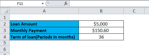
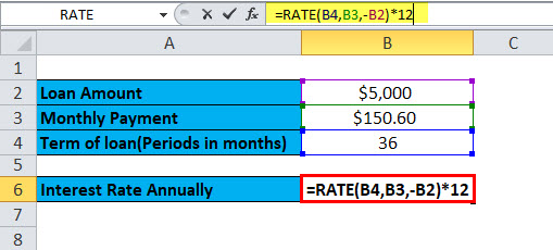
You want to buy a car. For this, you apply for a loan of $5,000 from the bank. The bank provides this loan for 5 years and fixed the monthly payment amount of $150.60. Now you need to know the annual interest rate.
Here, we have the following information available:
=RATE (B4, B3,-B2)
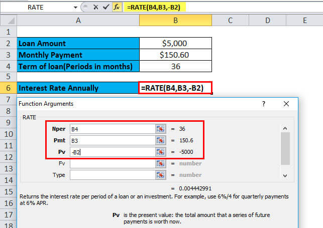
Here the result of the function is multiplied by 12, which gives the annual percentage rate. B2 is a negative value because this is an outgoing payment.
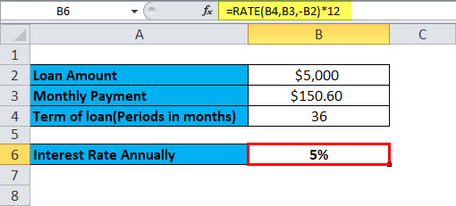
=RATE (B4,B3,-B2)*12
The annual percentage rate will be:
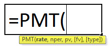
PMT (Payment)
This function is used to calculate the payment made on every month for a loan or an investment on the basis of a fixed payment and constant rate of interest.
PMT Formula:
Example #2
You want to buy a house which costs $350,000. To buy this, you want to apply for a bank loan. The bank offers you the loan at an 18% annual interest rate for 10 years. Now you need to calculate the monthly installment or payment of this loan.
Here, we have the following information available:
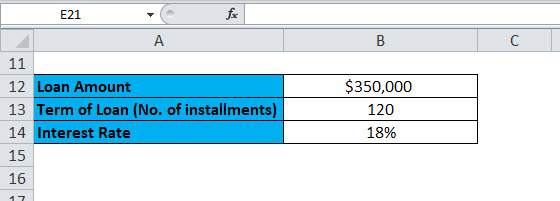
The interest rate is given annually, hence divided by 12 to convert to a monthly interest rate.
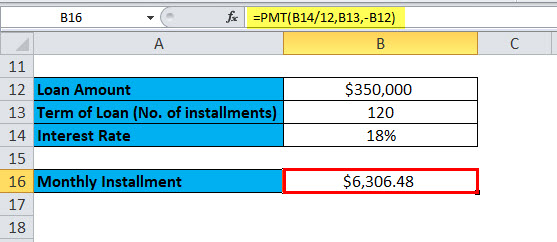
=PMT (B14/12,B13,-B12)
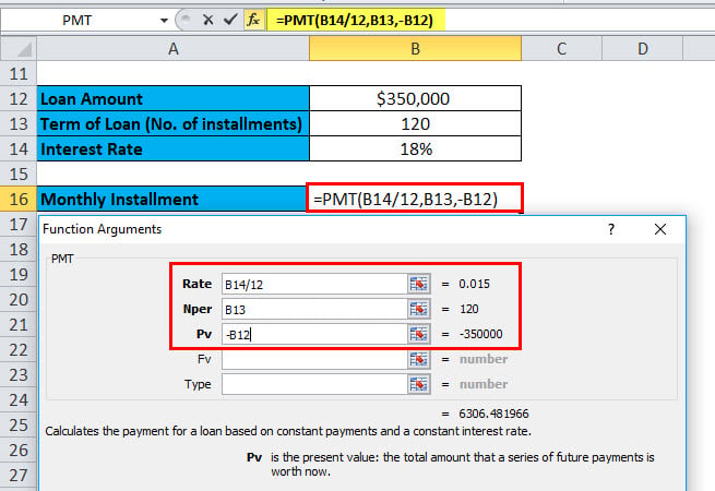
The Result will be:
PV (Present Value)
This function calculates the present value of an investment or a loan taken at a fixed interest rate. Or in other words, it calculates the present value with constant payments, or a future value, or the investment goal.
PV Formula:
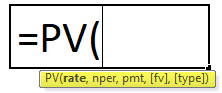
Example #3
You have made an investment that pays you $200,000 after 18 years at an annual interest of 9%. Now you need to find out how much to be invested today to get a future value of $200,000.
Here, we have the following information available:
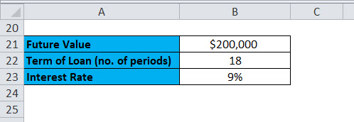
=PV (B23,B22,0,B21)
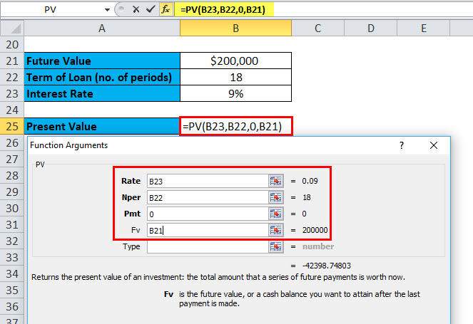
Result is:
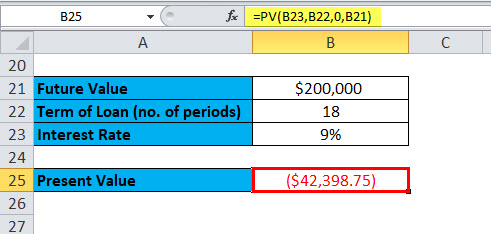
The result is in negative numbers as it’s the cash inflow or incoming payments.
Let’s take one more example of the PV function.
Example #4
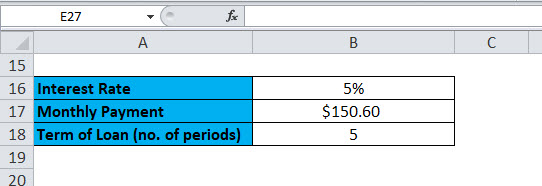
You have taken a loan for 5 years that has a fixed monthly payment amount of $150.60. The annual interest rate is 5%. Now you need to calculate the original loan amount.
Here, we have the following information available:
=PV (5/12,5*12,-B17,0)
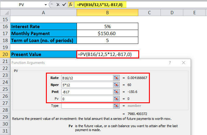
Result is:
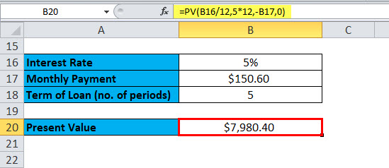
This monthly payment was rounded to the nearest penny.
FV (Future Value)
This function is used to determine the future value of an investment.
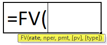
FV Formula:
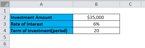
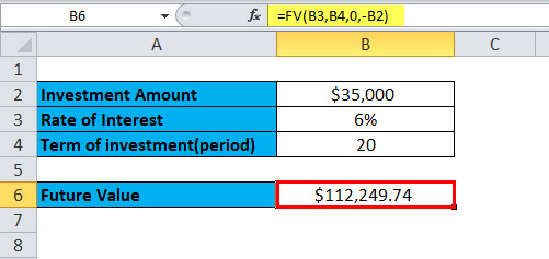
Example #5
You invest a certain amount of money, $35,000 at 6% annual interest for 20 years. Now the question is: with this investment, how much will we get after 20 years?
Here, we have the following information available:
=FV (B3,B4,0,-B2)
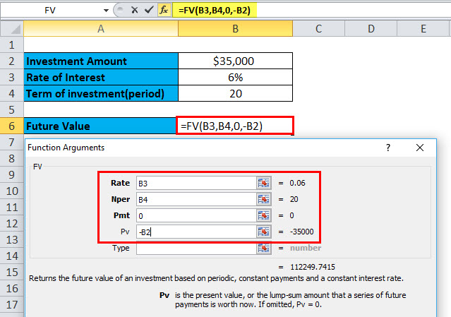
Result is :
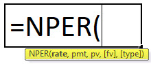
NPER (No. of periods)
This function returns the total no. of periods for invhttps://www.educba.com/nper-function-in-excel/stment or for a loan.
NPER Formula:
Example #6
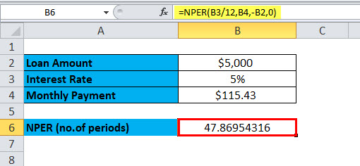
You take a loan of amount $5,000 with a monthly payment amount of $ 115.43. The loan has a 5% annual interest rate. To calculate the no. of periods, we need to use the NPER function.
Here, we have the following information available:
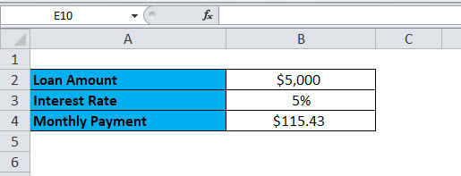
=NPER (B3/12,B4,-B2,0)
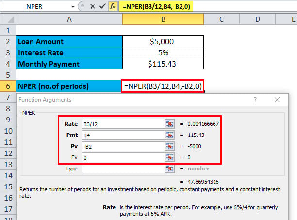
This function returns 47.869 i.e. 48 months.
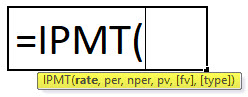
IPMT (Interest payment)
This function returns the interest payment of a loan payment or an investment for a specific time period.
IPMT Formula
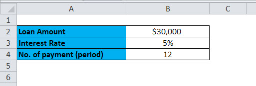
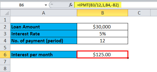
Example #7
You have taken a loan of $30,000 for one year at an annual interest rate of 5%. Now to calculate the interest rate for the first month, we will use the IPMT function.
Here, we have the following information available:
=IPMT(B3/12,1,B4,-B2)
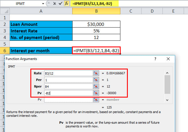
Result is:
Things to Remember
There are two factors commonly used by the finance industry – Cash outflow & Cash inflow.
Cash outflow: Negative numbers denote the outgoing payments.
Cash inflow: Positive numbers denote the incoming payments.
Recommended Articles
This has been a guide to the Excel RATE function. Here we discuss the RATE Formula and how to use the RATE function along with practical examples and a downloadable excel template. You can also go through our other suggested articles –
- Use of OR Function in MS Excel
- Use of NOT Function in MS Excel
- Use of AND Function in MS Excel
- Use of LOOKUP in MS Excel?