
Name a cell
-
Select a cell.
-
In the Name Box, type a name.

-
Press Enter.
To reference this value in another table, type th equal sign (=) and the Name, then select Enter.
Define names from a selected range
-
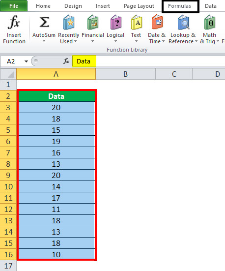
Select the range you want to name, including the row or column labels.
-
Select Formulas > Create from Selection.
-
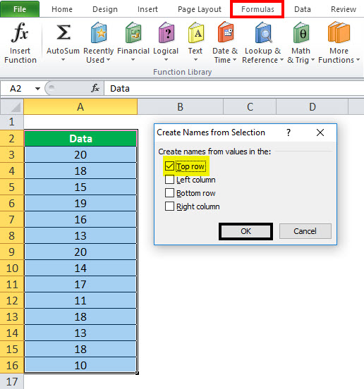
In the Create Names from Selection dialog box, designate the location that contains the labels by selecting the Top row, Left column, Bottom row, or Right column check box.
-
Select OK.
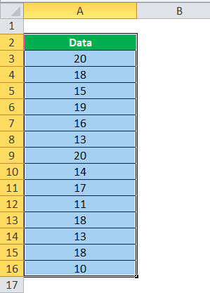
Excel names the cells based on the labels in the range you designated.
Use names in formulas
-
Select a cell and enter a formula.
-
Place the cursor where you want to use the name in that formula.
-
Type the first letter of the name, and select the name from the list that appears.
Or, select Formulas > Use in Formula and select the name you want to use.
-
Press Enter.
Manage names in your workbook with Name Manager
-
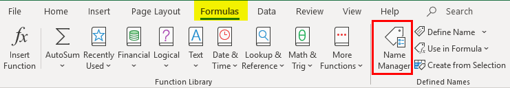
On the ribbon, go to Formulas > Name Manager. You can then create, edit, delete, and find all the names used in the workbook.
Name a cell
-
Select a cell.
-
In the Name Box, type a name.
-
Press Enter.
Define names from a selected range
-
Select the range you want to name, including the row or column labels.
-
Select Formulas > Create from Selection.
-
In the Create Names from Selection dialog box, designate the location that contains the labels by selecting the Top row,Left column, Bottom row, or Right column check box.
-
Select OK.
Excel names the cells based on the labels in the range you designated.
Use names in formulas
-
Select a cell and enter a formula.
-
Place the cursor where you want to use the name in that formula.
-
Type the first letter of the name, and select the name from the list that appears.
Or, select Formulas > Use in Formula and select the name you want to use.
-
Press Enter.
Manage names in your workbook with Name Manager
-
On the Ribbon, go to Formulas > Defined Names > Name Manager. You can then create, edit, delete, and find all the names used in the workbook.
In Excel for the web, you can use the named ranges you’ve defined in Excel for Windows or Mac. Select a name from the Name Box to go to the range’s location, or use the Named Range in a formula.
For now, creating a new Named Range in Excel for the web is not available.
What is Name Range in Excel?
The name range in Excel is the range that has been given a name for future reference. To make a range as a named range, select the range of data and then insert a table. Then, we put a name to the range from the Name Box on the left-hand side of the window. After this, we can refer to the range by its name in any formula.
The name range in Excel makes it much cooler to keep track of things, especially when using formulas. You can assign a name to a range. No problem with any change in that range; you need to update the range from the Name Manager in ExcelThe name manager in Excel is used to create, edit, and delete named ranges. For example, we sometimes use names instead of giving cell references. By using the name manager, we can create a new reference, edit it, or delete it.read more. You do not need to update every formula manually. Similarly, you can create a name for a formula. Then, if you want to use that formula in another formula or another location, refer to it by name.
- The name ranges are significant because you can put any names in your formulas without considering cell references/addresses. Furthermore, you can assign the range with any name.
- Create a named range for any data or a named constant and use these names in your formulas in place of data references. In this way, you can make your formulas easier to comprehend better. A named range is just a human-understandable name for a range of cells in Excel.
- Using the name range in Excel, you can simplify and comprehend your formulas better. For example, you can assign a name for a range in an excel sheet for a function, a constant, or table data. Once you start using the names in your Excel sheet, you can easily understand these names.
Table of contents
- What is Name Range in Excel?
- Define Names For a Selected Range
- Excel names the cells based on the labels in the range you designated.
- Update named ranges in the Name Manager (Control + F3)
- How to Use Name Range in Excel?
- Example #1 Create a name by using the Define Name option
- Example #2 Make a named range by using Excel Name Manager
- Name Range using VBA.
- Things to Remember
- Recommended Articles
- Define Names For a Selected Range
Define Names For a Selected Range
- Select the data range you want to assign a name, then select formulas and create from the selection.
- Click on the “Create Names from Selection,” then select the “Top row,” “Left column,” “Bottom row,” or “Right column” checkbox and select “OK.”
Excel names the cells based on the labels in the range you designated.
- Use names in formulas, then select a cell and enter a formula.
- Place the cursor where you want to use the name range formula.
- Type the first letter of the name, and select the name from the list that appears.
- Or, select “Formulas,” then use in formula and select the name you want to use.
- Press the “Enter” key.
Update named ranges in the Name Manager (Control + F3)
You can update the name from the Name Manager. Press “Ctrl” and “F3” to update the name. Select the name you want to change, then change the reference range directly.
How to Use Name Range in Excel?
Let us understand the working of conditional formatting by simple Excel examples.
You can download this Using Names in Excel Template here – Using Names in Excel Template
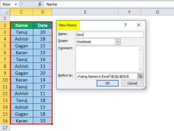
Example #1 Create a name by using the Define Name option
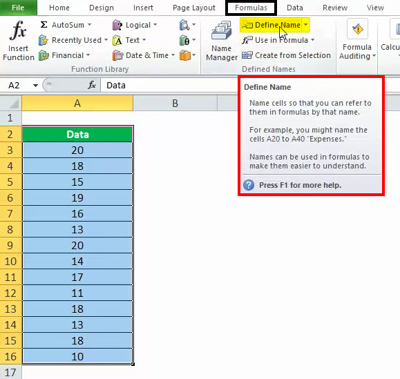
Below are the steps to create a name by using the “Define Name” option:
- First, select the cell(s).

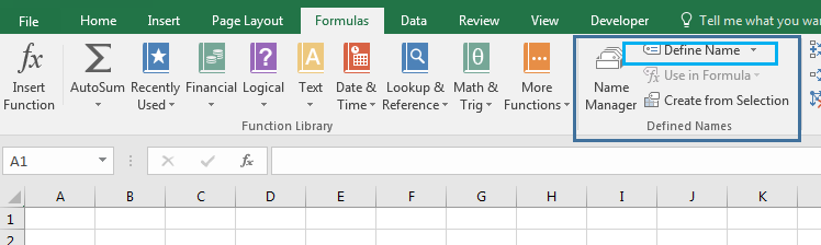
- On the “Formulas” tab, click the “Define Name” in the “Defined Names” group.

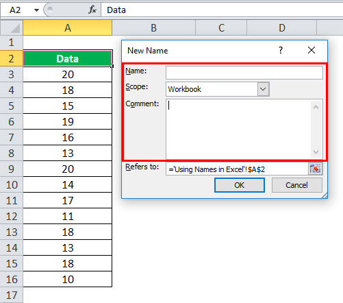
- In the “New Name” dialog box, specify three things:

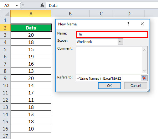
- First, in the “Name” box, type the range name.

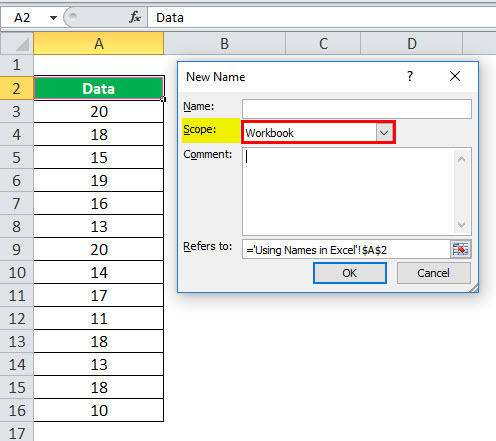
- In the “Scope” drop-down, set the name scope (Workbook by default).

- In the “Refers to” box, check the reference and correct it if needed. Finally, click “OK” to save the changes and close the dialog box.


Example #2 Make a named range by using Excel Name Manager
- Go to the “Formulas” tab, then the “Defined Names” group, and click the “Name Manager” or press “Ctrl + F3” (the preferred way).
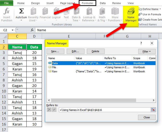
- In the top left-hand corner of the “Name Manager” dialog window, click the “New… button:”
Name Range using VBA.
We can apply the naming in VBA; here is the example as follows:
Sub sbNameRange()
‘Adding a Name
Names.Add Name:=”myData”, RefersTo:=”=Sheet1!$A$1:$A$10″
‘OR
‘You can use Name property of a Range.
Sheet1.Range(“$A$1:$A$10”).Name = “myData”
End Sub
Things to Remember
We must follow the below instruction while using the name range.
- The names can start with a letter, backslash (), or an underscore (_).
- The name should be under 255 characters long.
- The names must be continuous and cannot contain spaces and most punctuation characters.
- There must be no conflict with cell references in names using in excelCell reference in excel is referring the other cells to a cell to use its values or properties. For instance, if we have data in cell A2 and want to use that in cell A1, use =A2 in cell A1, and this will copy the A2 value in A1.read more.
- We can use single letters as names, but the letters “r” and “c” are reserved in Excel.
- The names are not case-sensitive – “Tanuj”, “TANUJ”, and “TaNuJ” are all the same in Excel.
Recommended Articles
This article is a guide to the Name Range in Excel. We discuss using names in Excel, practical examples, and downloadable Excel templates here. You also may look at these useful functions in Excel: –
- VBA RangeRange is a property in VBA that helps specify a particular cell, a range of cells, a row, a column, or a three-dimensional range. In the context of the Excel worksheet, the VBA range object includes a single cell or multiple cells spread across various rows and columns.read more
- Data Tables ExcelA data table in excel is a type of what-if analysis tool that allows you to compare variables and see how they impact the result and overall data. It can be found under the data tab in the what-if analysis section.read more
- Data Validation using ExcelThe data validation in excel helps control the kind of input entered by a user in the worksheet.read more
- Paste SpecialPaste special in Excel allows you to paste partial aspects of the data copied. There are several ways to paste special in Excel, including right-clicking on the target cell and selecting paste special, or using a shortcut such as CTRL+ALT+V or ALT+E+S.read more
In this article, we will learn How to use Names in a Formula in Excel.
Scenario :
While working on Excel, you’ve must have heard about named ranges in excel. Maybe from a friend, colleague or some online tutorial. I have mentioned it many times in my articles. In this article we will learn about Named Range in Excel and will explore each and every aspect of it.
Named Ranges in Excel
Formulas -> Name Manager -> Define Name
Well, named ranges are nothing but some excel ranges that are given some meaningful name. For example if you have a cell say B1, containing everyday targets, you can name that cell as specifically “Target”. Now you can use “Target” to refer at A1 instead of writing B1.
In a nutshell, Named range is just naming of ranges.
How to name a range in Excel?
Define name manually:
To define a name to a range you can use shortcut CTRL + F3. Or you can follow these steps.
Now you can refer to it by just typing its name.
There are some rules to follow while creating names. Here are some.
- Names should not start from digits or special characters other than underscore (_) and backslash().
- Names can’t have spaces and any special characters except _ and .
- Range should not be named as cell references. For example A1, B1 or AZ100 etc.
- You can’t name a range as “r” and “c” because they are reserved for row and columns references.
- Two named ranges can’t have the same name in a workbook.
- Same range can have multiple names.
Well most of the time you will be working with structured data tables. They will have column and rows with column headings and row headings. And most of the time these names are meaningful to the data and you’d like to name your range as these column headings. Excel provides a tool to automatically name ranges using headings. Follow these steps.
Now each column is named as their heading. Whenever you type a formula, these names will be listed as options which can be accessed.
When we tablise a data in excel using CTRL + T, the column heading automatically is assigned as the name of the respective column. You should explore Excel Tables and their benefits.
Well there will be times when you would like to see all available named ranges in the workbook. To see all name ranges Press CTRL+F3. Or you can go to Formula Tab > Name Manager. This will list all named ranges that are available on the workbook. You can Edit available named ranges, delete them, add new names.
One Range Multiple Names
Excel allows users to name the same range with different names. For example range A2:A10 can be named ‘Customers’ and ‘Clients’ both at same time. Both names will refer to the same range A2:A10.
But you can’t have the same names for two different ranges. This is good. This eliminates the chance of ambiguity.
Get List of Named Ranges on Sheet
So if you want to have a list of named ranges and the ranges they are covering you can use this shortcut for pasting them in place in a sheet.
- Select a cell where you want to get a list of named ranges.
- Press F3. This will open a paste list dialogue box.
- Click on the paste list button.

- The list will be pasted on selected cells and onwards.


If you double click on the named ranges name in the paste name box, they will get written as formulas in the cell. Try it.
Update Named Ranges Manually
Well when you insert a cell inside a named range it updates automatically and expands it. But if you add data at the end of the table, you’ll need to update the named range. To update Named Ranges follow these steps.
- Press CTRL+F3 to open the name manager.
- Click on the named range that you want to edit. Click on Edit.
- In Refers to column type the range to which you want to expand and hit OK.
And It’s done. This is manual updating of named ranges. However, we can make it dynamic by using some formulas.
Update Named Ranges Dynamically
It is wise to make your named ranges dynamic so that you don’t have to edit them whenever your data overflows the predefined range.
I have covered it in a separate article called Dynamic Named ranges. You can learn and understand the benefits of it in detail here.
Deleting Named Ranges
When you delete the sum part of the named range, it auto adjusts its range. But when you delete the whole name range vanishes from the name list. Any formula, dependent on those ranges will show #REF error or they will give incorrect output (counting functions).
For any reason, if you want to delete named ranges, just follow these steps.
- Press CTRL+F3. Name manager will open.
- Select Named Ranges that you want to delete.
- Click on the Delete button or hit Delete button on keyboard.

Caution: Before you delete the named ranges make sure that no formulas are dependent on these names. If there is any, convert them to ranges first. Otherwise you’ll see #REF error.
Deleting Names with Errors
Excel provides tools to delete names that have errors only. You don’t need to identify each of them by yourself. To delete names with errors, follow these steps:
- Open Name Manager (CTRL+F3).
- Click on Filter drop down on right- upper corner.
- Select “Name with Errors”

- Select All and hit the delete button.

And they are gone. All the names with errors will be deleted from record immediately.
Named Ranges With Formulas
Best use of named ranges are explored with formulas. The Formulas get really flexible and readable with Named ranges. Let’s see how.
Easy To Write Formulas
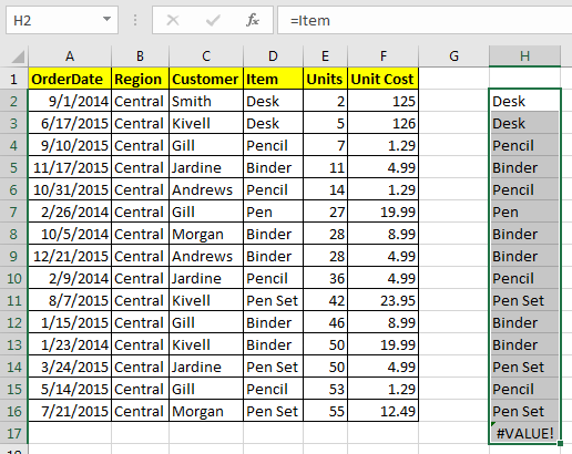
Now let’s say you have named a range as “Items”. Now the Items list you want to count “Pencils”. With names it is easy to write this COUNTIF formula. Just write
=COUNTIF(Item,»Pencil»)
As soon as you write the opening parenthesis of formula the list of available named ranges will appear
Without name you would write a give a range to COUNTIF function of Excel, for which you may have to look at the range first then select the range or type it in formula.
Excel Serves the Available Name Ranges.
The named ranges are shown as suggestions when you type any letter. As excel shows the list of formulas. For example if you type =u, each formula and named range will be displayed starting with u, so that you can use them easily.

Make Constants using Named Ranges
So far, we learned about naming ranges but you can actually name values too. For example if your client name is Sunder Pichai then you can make a name “Client” and it refers to write “Sundar Pichai”. Now whenever you will write =Client in any cell it will show Sundar Pichai.


Not only text, but you can also assign numbers as constant to work with. For example, you define a target. Or the value of something that will not change.
Absolute and Relative Referencing with Named Ranges
The referencing with Named ranges in is very flexible. For example if you write the name of a named range in a relative cell to the named range, it will behave like a relative reference. See below image.
But when you use it with formulas it will behave as absolute. Well most of the time you’ll be using them with formulas, so you can say that they are by default Absolute but actually they are flexible.

But we can make them relative too.
How to make Relative Named Ranges in Excel?
Let’s say if i want to name a range “Befor” which will refer to cell left to wherever it is written. How do I do that? Follow these steps:
- Press CTRL+F3
- Click on New
- Type “Befor” in the ‘Name’ Section.
- In ‘Refers to:’ section write address of cell in left. For example if you are in cell B1 then write “=A2” in ‘Refers to:’ section. Make sure that it does not have a $ sign.

Now wherever you will write the “Befor” in formula, it will refer to cell left to it.

Here, I used it before in the COLUMN function. The formula returns the column number of the left cell where it is written. To my suprise, A1 shows the column number of the last column. Which means the sheet is circulare. I thought it will show an #REF error.
Give Name to Often Used Formulas?
Now this one is amazing. Many times you use the same formula again and again in a worksheet. For example you may want to check if a name is in your customer list or not. And this need may occur many times. For this you’ll write same complex formula every time.
=IF(COUNTIF(Customer,I3),»In List»,»Not in List»)
How about, if you just type ‘=IsInCustomer’ in a cell and it will show you if the value in the left cell is in the customer list or not?

For example, I have prepared a table here. Now i just want to type “=IsInCustomer” in J5 and i would like to see if the value in I5 is in the Customer list or Not. To do so follow these steps.
- Press CTRL+F3
- Click on New
- In Name write, ‘IsInCustomer”
- In ‘Refers To’ write your formula. =IF(COUNTIF(Customer,I5),»In List»,»Not in List»)

- Hit the OK button.

Now wherever you type ‘IsInCustomer’, It will check the value in the left cell in the Customer list.

This stops you from repeating yourself again and again.
Apply Named Ranges to Formulas
So many times, we define names to our ranges after we have already written formulas based on ranges. For example I have Total Price as Cells =E2*F2. How can we change it to Units*Unit_Cost.
- Select the formulas.
- Go to the formula tab. Click on Define Name drop down.

- Click on Apply Names.
- List of all named ranges will appear. Choose the right names and hit ok.


And the names are now applied. You can see it in the formula bar.

Easy to Read Formulas with Named Ranges
As you’ve seen that named ranges make it easy to read the formulas. If I write =COUNTIF(“A2:A100”,B2), no one will understand what I am trying to count, until they see the data or someone explains it to them.
But if I write =COUNTIF(region,’east’), most users will immediately get it that we are counting occurrences of ‘east’ in the region named range.
Portable Formulas
Named ranges make it very easy to copy and paste formulas without worrying about changing references. And you can take one formula from one workbook to another and it will work fine until and unless the destination workbook has the same name.
For example if you have a Formula =COUNTIF(region,east) in the Distribution Table and you have another workbook say customers that also has a named range “Region”. Now if you copy this formula directly anywhere on that workbook it will show you correct information. The structure of data will not matter. It doesn’t matter where the hell is that column in your workbook. This will work correctly.

In the above image I have used the exact same formula in two different files to count the number or east occuring in the region list. Now they are in different columns but since both of them are named as regions it will work perfectly.
Navigate Easily in Workbook
It gets easier to navigate in a workbook with named ranges. You just need to type the name of the name in the name box. Excel will take you to the range, doesn’t matter where you are in the workbook. Given that named range is of Workbook scope.
For example, if you are on sheet10 and you want to get a customer list, and you don’t know on which sheet it is. Just go to name box and type ‘customer’. You’ll be directed to the named range in fraction of a second.

It will reduce the effort of remembering the ranges.
Navigate Using Hyperlinks with Named Range
When your sheet is large and you often go from one point to another, you like to use hyperlinks to navigate easily. Well Named Ranges can work perfectly with Hyperlinks. To add hyperlinks using named ranges follow these steps.
And it’s done. You have your hyperlink to your chosen named range. Using this you can create an index of named ranges that you can see and click to navigate to them directly. This will make your workbook really user friendly.
Named Range and Data Validation
Named ranges and Data Validation is kind of made for each other. Named ranges make data validation highly customisable. It gets a lot easier to add a validation from a list using named range. Let us see how..
- Go to Data tab
- Click on Data Validation
- Select List in ‘Allow:’ section
- In ‘Source:’ section, type “=Customer” (write whichever named range you have)

- Hit OK

Now this cell will have names of customers who are part of the Customer named range. Easy, isn’t it.
Dependent or Cascading Data Validation with Named Ranges
Now what if you want a cascading or dependent data validation. For example, if you want a drop down list that has categories, Fruits and Vegetables. Now if you choose fruits then another dropdown should show only fruits option and if you choose Vegetable then only vegetables.
This can be easily achieved by using Named ranges. Learn how.
- Dependent Drop down using Named Range
- Other Ways for Cascading Data Validation
Hope this article about How to use Names in a Formula in Excel is explanatory. Find more articles on naming ranges and related Excel formulas here. If you liked our blogs, share it with your friends on Facebook. And also you can follow us on Twitter and Facebook. We would love to hear from you, do let us know how we can improve, complement or innovate our work and make it better for you. Write to us at info@exceltip.com.
Related Articles :
The Name Box in Excel : Excel Name Box is nothing but a small display area on top left of excel sheet that shows the name of active cell or ranges in excel. You can rename a cell or array for references.
How to Get Sheet name of worksheet in Excel : CELL Function in Excel gets you the information regarding any worksheet like col, contents, filename, ..etc. Learn how to get the sheet name using the CELL function here.
How To Get Sequential Row Number in Excel : Sometimes we need to get a sequential row number in a table, it can be for a serial number or anything else. In this article, we will learn how to number rows in excel from the start of data.
Increment a number in a text string in excel : If you have a large list of items and you need to increase the last number of the text of the old text in excel, you will need help from the two TEXT and RIGHT functions.
Popular Articles :
How to use the IF Function in Excel : The IF statement in Excel checks the condition and returns a specific value if the condition is TRUE or returns another specific value if FALSE.
How to use the VLOOKUP Function in Excel : This is one of the most used and popular functions of excel that is used to lookup value from different ranges and sheets.
How to use the SUMIF Function in Excel : This is another dashboard essential function. This helps you sum up values on specific conditions.
How to use the COUNTIF Function in Excel : Count values with conditions using this amazing function. You don’t need to filter your data to count specific values. Countif function is essential to prepare your dashboard.
Hi everyone. In this post, I’ll describe how to use names within Microsoft Excel.
Names are one of the most powerful, and one of the least utilized features in Excel. In this post, I’ll describe some of the different types of names that are available in Microsoft Excel, and get into some advanced features of names.
There are two types of categories of names: Names that refer to ranges, and names that don’t. And there are three different types of names: named ranges, named constants, and named formulas. Named ranges always refer to ranges; named constants never refer to ranges; and named formulas may or may not refer to ranges. Before I start describing the different types of names, I quickly want to discuss the name manager.
Name manager
The name manager is where you can create, edit, and delete any of the names you’ve created. To get to the name manager, you click the formulas tab on the ribbon, and then click name manager. You can click new to create a new name, edit to edit an existing name (or double click an existing name), and delete to delete a name. Next I’ll describe named ranges.
Named ranges
A named range is a custom word that refers to a cell or a range of cells within a particular worksheet in a workbook. You can create named ranges in a number of different ways:
-
After you select a cell, or a range of cells, you can type a name into the name box (it’s on the left most side where the formula bar is located), hit enter, and Excel will create the name.
-
You can click on the formulas tab on the ribbon, click define name, enter a word for the name, and then select the cell or range of cells, and click OK
-
If the cell or range of cells have headers, you can also use the headers as their name (assuming they’re not reserved keywords in Excel.) Highlight the cell or range of cells you want to refer to, including the headers. Then click the formulas tab on the ribbon, and click the ‘Create from Selection.’ Excel will try to guess where the headers are located for the name. If it is correct, click OK and you will have names that refer to the values that the headers are adjacent to.
Once you’ve created named ranges, you can substitute them anywhere you’d use regular range references. So you could write:
=SUM(2014sales)
rather than writing :
=SUM('2014 Sales'!$C$1:$C$12)
Or you could write
=VLOOKUP(A1, salesdata, 2, false)
rather than:
=”VLOOKUP(A1,’Sheet 1’!$B$1:$B$20, 2, false.)
It’s important to note that, by default, named ranges are created using absolute references (this will be important later when we talk about named formulas.) Next I’ll talk about named constants.
Named constants
As I said earlier, named constants never refer to ranges in Excel. They don’t exist anywhere within the worksheet, but exist purely in memory. Instead of referring to ranges, they refer to a particular value. Unlike a named range, where the name would refer to whatever values are in that range, a named constant always refers to the same value. There are a few different types of names constants. In this section I’ll discuss names that refer to numbers, names that refer to text, names that refer to Boolean values, and names that refer to arrays. I’ll describe each of them briefly.
To create a named constant, you click the formulas tab on the ribbon, and click define name. After you’ve entered a name for your constant, click the “refers to” portion where the formula is. Select the sheet name, and overwrite it with the value you’d like to replace. These names constants follow the same rules as regular Excel formulas.
-
If you want to use text, it must be enclosed in double quotes e.g. =”Hello world!”
-
For numbers you can just use the value e.g. =12345
-
For Boolean values, quotes are not required e.g. =TRUE
-
For arrays, they must be written with brackets and the requisite commas or semicolons. e.g. «={1,2,3,4,5}». And when you call them from the worksheet, you must select a range of cells that’s the same length as number of elements in the array (e.g. A1:E1), use the name in a formula, and hit ctrl + shift + enter.
Now that I’ve described named ranges and constants, I’ll describe named formulas, which are the most powerful way to use names.
Named formulas
Named formulas are names that refer to formulas within Excel. Typically, this will be some combination of ranges, Excel worksheet functions, values, and even other names.
You create named formulas in the same way that you create the named constants. When you go to the ‘refers to’ section, I would STRONGLY recommend immediately pressing F2. By default, the dialog box uses the arrow keys to shuffle through ranges in the Excel worksheet. So you have to hit F2 to go into edit mode and move around within the ‘refers to’ section.
You can create a name called SumA that refers to the formula:
=SUM(‘Sheet 1’!A:A)
Or you can create a name called vlook that refers to the formula:
=VLOOKUP(‘Sheet1’!$A$1,’ Sheet1’!$B:$C,2,false).
A feature of names that you can utilize when you create them is their scope. Scope refers to where you’re able to call the names. You can either limit them to only be used within a particular sheet, or set them at the workbook level so that they can be used from any sheet within the workbook they’re defined in. Names by default will only refer to the sheets of the ranges they’re defined in. So if you set a name to workbook level, and it refers to range A:A in Sheet 1, if you use that name in a formula in Sheet 3, it will still refer to the range A:A in Sheet 1. This is because the name ‘Sheet 1’ is defined in the name. However, you can create names that refer to the ranges in the activesheet. You do this by deleting the name of the sheet in the formula (but you must leave in the exclamation point). So, if you change:
=’Sheet 1’!$A:$A
to
=!$A:$A
it will refer to the range A:A in the sheet the name is called from.
As I noted earlier, names by default come with with absolute reference. But you can shift them to relative references by selecting the range in the ‘refers to’ section and clicking F4 to change their reference type. You might be wondering why you’d want to do this. Well, let’s say I create a name called Summy that refers to the formula:
=SUM(!A1:A2)
If I call this name from A3, it will sum the values in A1 and A2. But if I call it from B3, it will sum the values in B1 and B2. And since I wrote this name without a reference to a sheet, it will work in this way for any sheet within the workbook (assuming the scope is workbook level.)
One of the most advanced usages of names is creating named formulas with relative and absolute references. But this is tricky to do. For example, you can write a named formula like vlook that refers to the name:
=VLOOKUP(!A1,’Sheet 1’!$A:$C,3,false).
And you can use this formula to perform a vlookup function with these paramaters from any sheet within the workbook (assuming the scope is workbook level.) However, you have to be careful when you create names like this. Excel defines the relative reference from the active cell within the active sheet. So, if you write this formula from cell E1, for example, you’re telling Excel to lookup the value in the current row, four columns to the left (where A1 would be), and perform a vlookup with these paramaters. For my purposes, when I want to lookup a value to the immediate left of my name, I write a formula like this in cell B1.
Cons to using names
I hope I’ve shown you how powerful names are. You might be wondering at this point why more people don’t use names given their power and flexibility. One reason may be that they’re really easy to break. If a name refers to a particular range, and you delete it, that name will return a #REF error and will no longer work. You’d have to edit out the #REF errors or rewrite the name to get it working again. Although names are easy to break, there are a few ways to mitigate this:
-
Always use clear contents instead of delete rows for rows that are referenced by names.
-
Record a macro of you writing your names, and save it to your personal macro workbook. If one or several of your names break, simply delete the names and rerun the macro.
-
Alternatively, instead of using ranges, you can use other names as substitutes for the ranges. So you could write a name vlook like “=VLOOKUP(val,rang, 2, false)” where val is another name that would refer to a lookup parameter (e.g. “A”) and rang is another name that would refer to a lookup range like “$A:$B”. If you write your names this way, they will not break. Since these names don’t directly refer to a particular range, they won’t break when any range is deleted. But this is a bit tedious and requires you to create, edit, and manage more names. (I personally use a combination of the first and second approach.)
Another reason is that names, especially named formulas, can be quite difficult to write. You must be very careful when you named formulas. If you did not write everything exactly as it should be written, the name may not function as intended. Even for someone like me, it may take me a few tries to get everything correct when I’m writing a name. But I think the pros of using names far outweigh their cons.
Other topics / using names with indirect
Since this is a rather long post now, I’ll end it here. I would like to mention some things I didn’t discuss in case you’d like to look into them yourselves.
You can use a named formula with the indirect function to accept dynamic parameters. So you can use:
=SUM(INDIRECT(!$D$1))
in a name and enter a range in D1 to sum whatever range you enter into D1.
You can use names with data validation and the indirect function to create a double data validation where a value from the first data validation limits the values in the second data validation (Excel Is Fun has a video describing this.)
I hope you’ve all learned something useful and will start utilizing the power of names within Excel!
Excel Name Box (Table of Contents)
- How to Give Name in Name Box?
- How to Edit and Delete the Name of the Data Range?
- How to Use the Name Box in Excel?
Definition of Name Box in Excel
The box located to the left side of the formula bar which addresses the selected cell or group of cells in the spreadsheet is called Name box. In the below screenshot highlighted with a red color box is the Name box.
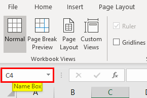
This Name box helps to address the group of cells with a name instead of addressing rows and columns combination. This tutorial will cover how to create a Name box and how to use it while working with data.
How to Give Name in Name Box?
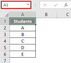
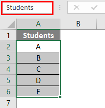
Consider a small example of student’s data like below. In the below screenshot Name box representing the selected cell A1.
Now we will select the student data alone from the table, excluding the header “Students”.
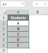
After selecting the data, go to the name box and type the name which you want to name the data range. Here I am giving the data range name as “Students”. After Inputting the name Press Enter Key, it will create the name.
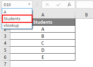
Now, whenever we want to select the student’s data range, we can select from the Name box drop down as below.
If we add the marks data of the students as below.
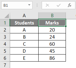
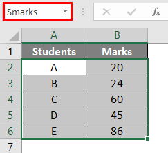
We already gave the name “students” to column A data. Still, we can give the name to the combined data of students and marks as “Smarks”.
How to Edit and Delete the Name of the Data Range?
We have seen how to give a name to the data range. Now, we will see how to edit and delete the name.
#1 – Edit the Name of the Data Range
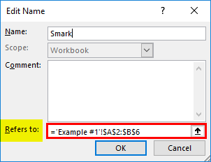
In case if we incorrectly input the name or want to change the name. We gave the name as “Smakrs” for the student data range incorrectly, which should be “Smarks”. Now, we will change the name from “Smakrs” to “Smarks.”
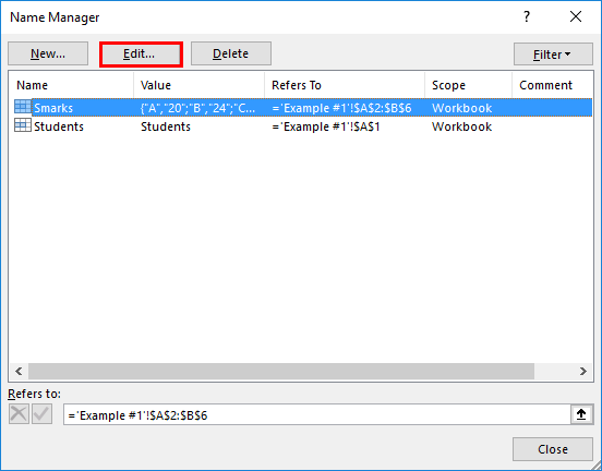
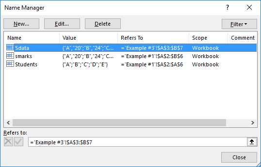
The name box does not have the option to edit the given name; we should change the name in “Name Manager” under the “Formulas” menu. Click on the “Name Manager” to view the available names.
Click on the option “Edit” on the top.
So that we will get the below “Edit Name” box.
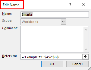
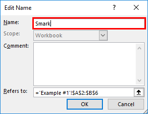
Edit the name to “Smark” as required.
In case if we want to increase or decrease the range of cells, we can change in “Refers to” option.
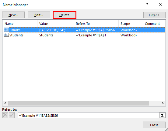
#2 – Deleting the Name of the Range
It is as similar to how we edit the name. Click on the “Name Manager”. Select the name of the range which we want to delete. Click on the “Delete” option on the top.
This is how we will create, Edit, and Delete the Name in the name box.
How to Use the Name Box in Excel?
Let us understand how to use the name box with a few examples.
You can download this Name Box Excel Template here – Name Box Excel Template
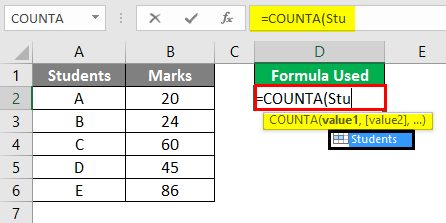
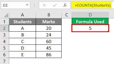
Example #1 – Count Formula with Name Box
Suppose we want to count the number of students from the student’s table. We can use the count formula with the name of the range. In the below screenshot, we input only the half name of the range then the system displays the name automatically. Select the name and close the formula.
Below you can see the output.
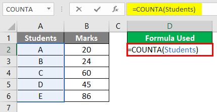
As the number of students is five, it should display 5. Remember, it is not COUNT; it is COUNTA formula.
Example #2 – SUM with the Name Box
Now we will see how to perform the SUM operation using the name feature. Our task is to sum the marks of all the students. In the SUM formula, we will give the range name “Smarks”, which we created earlier, instead of the range B2 to B6.
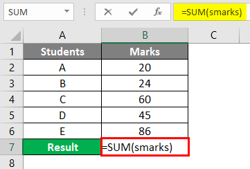
After using the formula, the output is shown below.
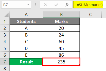
So, to replace the range address, we can use the name of the range. The name range will also pop up if we input the first few letters of the name range.
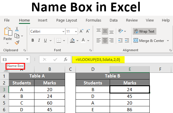
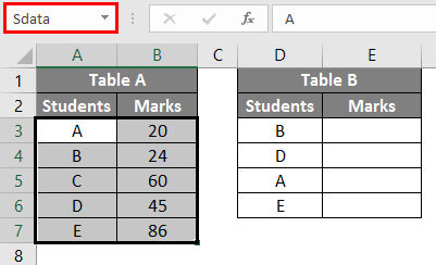
Example 3 – VLOOKUP with Name Box
We have to perform VLOOKUP for Table B to find the marks from Table A.
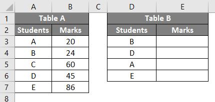
Create a name “Sdata” for data in Table A as below.
Now input the VLOOKUP Formula in Table B.
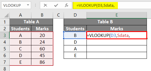
Once you select the “lookup_value” as E3, give the table array as “Sdata”, which is the name of data range from Table A as the range has 2 columns, input column index as 2, then input zero(for True).
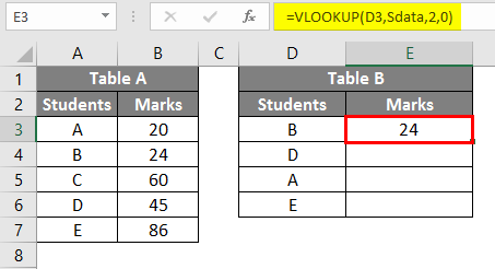
Expand the formula to get marks for other students.
Example #4 – Excel Name for Constant
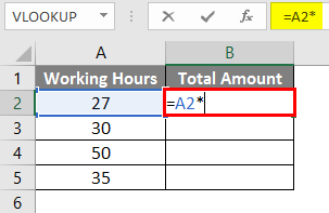
We can use the Excel name feature for creating constant also. We will see one example of this to understand in a better way. Consider a table having data of the number of hours of employees as below.
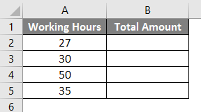
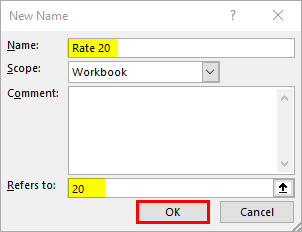
The charge per hour will be 20 rupees. So, we will create a constant with the value 20. Click on the Name formulas menu.
Click on the Name Manager, and the below window will appear.
Click on the “New” option, and it will take you to the below screen.
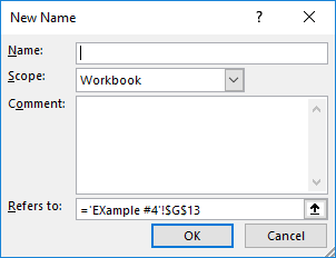
Give the name as Rate 20, and in “Refers to” give constant value 20 as below and click on OK.
Now go to our table and input the formula for multiplication with the use of name constant. Start the formula with the Equal symbol and select the number of hours option.
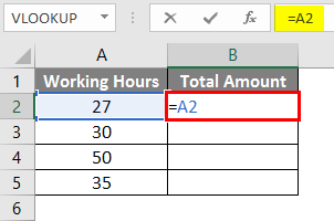
Add a Multiplication symbol.
Now give the constant name we created.
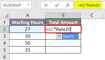
Select the Rate20 and Press Enter Key. It will multiply the number of hours by 20.
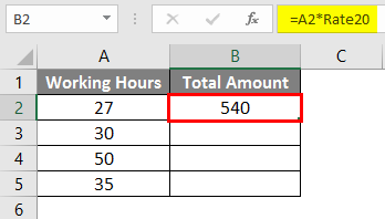
Drag the formula from cell B2 to B5.
Things to Remember About Name Box in Excel
- While giving the name for a range, make sure there should not be any spaces as it will not take if we input any spaces in between.
- Don’t include punctuations in the name.
- The name will be case sensitive; hence, it will be the same whether we give the name “Hai” or “hai”. While calling the range, you can use any case letters.
- The name should start with a letter or Backslash “” or Underscore “_”. Other than these, if the name starts with any other letter, Excel will throw you an error.
- The name can be applicable at sheet level or workbook level; it depends on our selection while creating the name in the name manager.
- The name should be unique as it will not allow duplicate values.
- The name can be a single character to Eg: “A”.
Recommended Articles
This is a guide to Name Box in Excel. Here we discuss how to use the Name Box in Excel along with practical examples and a downloadable excel template. You can also go through our other suggested articles –
- Count Names in Excel
- Excel Named Range
- VBA Name
- Combine First and Last Name in Excel
Download PC Repair Tool to quickly find & fix Windows errors automatically
Defining and using names in Formulas in Excel can make it easier for you and to understand data. Besides, it also serves as a more efficient way to manage the various processes that you create in your worksheets. So, in the following post, we will help you to define and use names in Excel formulas.
You can define a name for a cell range, function, constant, or table and once you become familiar with the technique, you can easily update, audit or manage these names. For this, you’ll first need to:
- Name a cell
- Use Create from selection option
The approach is useful if you want to reference it in a formula or another worksheet.
1] Name a cell
Let us say that we want to create a report of tax rates for different states.
Launch Excel and open a blank sheet.
Name the table as shown in the image and enter the values corresponding to the names.
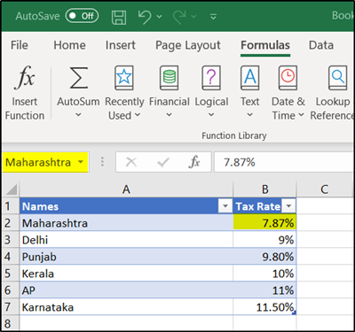
Next, to define a name for a cell select it. Then, select the name box (adjacent to the left side of the formula bar), type a name and press Enter.
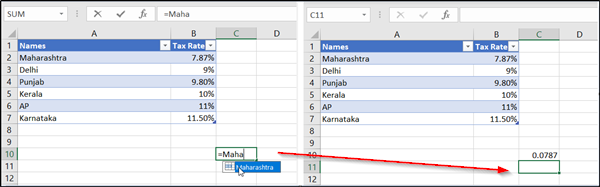
Now the cell has been named you can use it as a reference in the formula.
For instance, select a cell, put ‘=’ sign and the name you gave to the cell and press enter. You will notice that the data from the cell would appear there, replacing the name.
2] Use Name in formulas
You can also let Excel name a range or table cells for you.
For this, select the cells in the table you want to name.
Next, go to the ‘Formula’ tab on the ribbon bar and choose ‘Create from selection’ option.
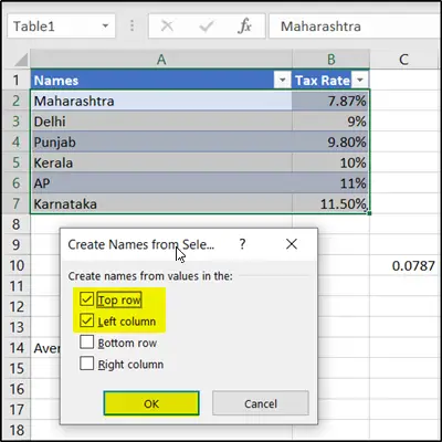
In the ‘Create from selection’ dialog box, choose the locations of any labels that are in the selected table and hit the ‘OK’ button.
Naming a range makes it easier to reference cells even on a different worksheet.

Wherever you are in your workbook, select a cell, type ‘=’ followed by any formula you would like to use followed by the name you defined for the cells.
That’s it, you should see the results displayed in the cell.
How to delete defined names in Excel
To delete Names in Excel:
- Open Formulas tab, in the Defined Names group
- Select Name Manager
- Next, click the name you want to delete
- Click Delete > OK.
That’s it!

A post-graduate in Biotechnology, Hemant switched gears to writing about Microsoft technologies and has been a contributor to TheWindowsClub since then. When he is not working, you can usually find him out traveling to different places or indulging himself in binge-watching.
Names in Excel VBA – Explained with Examples!
Names in Excel VBA makes our job more easier. We can save lot of time using Names. It is easy to maintain the formulas, Cells,Ranges and Tables. You can define the names once in the workbook and use it across the workbook. The following examples will show some of the Names daily operations.
- Adding Names in Excel VBA
- Deleting Names in Excel VBA
- Hide UnHide Names in Excel VBA
Adding Names in Excel VBA:
Sometimes you may need to Add name to a particular range in excel worksheet. We can manage range names in excel vba with using names collection.
- Solution
- Code
- Output
- Example File
Adding Names in Excel VBA – Solution(s):
We can use Names.Add method or Name property of a range for adding names in excel VBA.
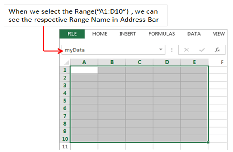
We can create range name in the following way. It contains several properties.We must define Name and the Refers To property.please find the following example.The following code creates a name “MyData” and referring to sheet1 of a range(“$A$1:$E$10”)
Code:
'Naming a range
Sub sbNameRange()

    'Adding a Name
    Names.Add Name:="myData", RefersTo:="=Sheet1!$A$1:$E$10"

    'OR

    'You can use Name property of a Range
    Sheet1.Range("$A$1:$E$10").Name = "myData"

End Sub
Output:

Instructions:
- Open an excel workbook
- Press Alt+F11 to open VBA Editor
- Double click on ThisWorkbook from Project Explorer
- Copy the above code and Paste in the code window
- Press F5
- GoTo Sheet1 and Select Range A1 to D10
- You should see the following example
Example File
Download the example file and Explore it.
Analysistabs – Adding Name to Range in excel Workboobk
Deleting Names in Excel VBA:
Sometimes you may need to Delete range name in existing excel workbook for cleaning broken references in excel workbook.
- Solution
- Code
- Output
- Example File
Deleting Names in Excel VBA – Solution(s):
You can use Delete method for deleting existing names in excel workbook.We can delete range name in the following way.please find the following example.The following code Deletes a name “MyData”.
Code:
'Deleting Names
Sub sbDeleteName()

    'myData=Sheet1.range("A1:E10")
    Names("myData").Delete

End Sub
Output:

Instructions:
- Open an excel workbook
- Press Alt+F11 to open VBA Editor
- Double click on ThisWorkbook from Project Explorer
- Copy the above code and Paste in the code window
- Press F5
- GoTo Sheet1 and Select Range A1 to D10
- You should see the following example
Example File
Download the example file and Explore it.
Analysistabs – Deleting Name to Range in excel Workboobk
Hide UnHide Names in Excel VBA:
Sometimes you may need to Hide UnHide names in Excel VBA.
- Solution
- Code
- Output
- Example File
Hide UnHide names in Excel VBA – Solution(s):
You Can Hide UnHide Names in Excel VBA using Visible Property in the following way. when we set visible proprty to false, We dont see defined range name . when we set visible proprty to true, We can see defined range name .
Code:
'Hiding a Name
Sub sbHideName()

	Names("myData").Visible = False

End Sub


'UnHide aName
Sub sbUnHideName()

	Names("myData").Visible = True

End Sub
Output:

Instructions:
- Open an excel workbook
- Press Alt+F11 to open VBA Editor
- Double click on ThisWorkbook from Project Explorer
- Copy the above code and Paste in the code window
- Press F5
- GoTo Sheet1 and Select Range A1 to D10
- You should see the following example
Example File
Download the example file and Explore it.
Analysistabs – Hide UnHide Names in excel Workboobk
A Powerful & Multi-purpose Templates for project management. Now seamlessly manage your projects, tasks, meetings, presentations, teams, customers, stakeholders and time. This page describes all the amazing new features and options that come with our premium templates.
Save Up to 85% LIMITED TIME OFFER

All-in-One Pack
120+ Project Management Templates
Essential Pack
50+ Project Management Templates
Excel Pack
50+ Excel PM Templates
PowerPoint Pack
50+ Excel PM Templates
MS Word Pack
25+ Word PM Templates
Ultimate Project Management Template
Ultimate Resource Management Template
Project Portfolio Management Templates
Related Posts
-
- Adding Names in Excel VBA:
- Adding Names in Excel VBA – Solution(s):
- Deleting Names in Excel VBA:
- Deleting Names in Excel VBA – Solution(s):
- Hide UnHide Names in Excel VBA:
- Hide UnHide names in Excel VBA – Solution(s):
VBA Reference
Effortlessly
Manage Your Projects
120+ Project Management Templates
Seamlessly manage your projects with our powerful & multi-purpose templates for project management.
120+ PM Templates Includes:
5 Comments
-
Eric W
April 30, 2015 at 11:17 AM — ReplyI am having a problem copying Ranges from one point to another in Excel using VBA.
I have tried several methods and get the same result any way I’ve tried
When the copy action is triggered, the destination has the copy from the header row in the destination
Example: Range(“U14:AO14”).Copy Destination:=Range(“A40”)
I am receiving the data from U2:AO2.
I have named the range by selection using the spreadsheet name window. The array that shows in the window shows the correct value. The destination is correct.Do you have a clue what is happening, or what I am doing wrong?
Thank You -
Amar
September 9, 2015 at 5:23 PM — ReplyCan this defined name be used for coding or in vba editor
-
PNRao
September 11, 2015 at 11:51 PM — ReplyHi Amar,
Yes! we can use the defined names in VBA. Example:Sheet1.Range("$A$1:$E$10").Name = "myData" Range("myData").Interior.ColorIndex = 3here, myData is a user defined name and the above code will change the background color of the defined range.
Thanks-PNRao! -
Silke Flink
September 12, 2015 at 12:35 AM — ReplyThank you for this post. I was wondering if it is possible to address a dynamic name range in VBA. I have a named range (though I use a lookup-function in the name manager) that is visible in the name manager and can be used in formulas in the Excel sheet.
I tried this
dim Taxes_from_Sales as Range
Set Taxes_from_Sales = Range(“Taxes_from_Sales”)whereas “Taxes_from_Sales” is a excel Lookup defined name range. VBA doesn’t recognize it cause of the formula.
Any idea how to approach this without writing Lookup in VBA?
Thanks for help
silke
-
PNRao
September 13, 2015 at 1:48 AM — ReplyHi,
It works for dynamic range. In your case, Lookup functions always returns a value, and we need a range to use in VBA.I have tried the below example and its working fine:
Sub DynamicNamedRange()
'Adding a dynamic Name
Names.Add Name:="test", RefersTo:="=OFFSET(Sheet1!$A$1,0,0,COUNTA(Sheet1!A:A),1)"

'Entering sample data
For i = 1 To 10
Cells(i, 1) = i
Next

'Formatting dynamic range
Range("test").Interior.ColorIndex = 3
End Sub
Thanks-PNRao!
Effectively Manage Your
Projects and Resources
ANALYSISTABS.COM provides free and premium project management tools, templates and dashboards for effectively managing the projects and analyzing the data.
We’re a crew of professionals expertise in Excel VBA, Business Analysis, Project Management. We’re Sharing our map to Project success with innovative tools, templates, tutorials and tips.
Project Management
Excel VBA
Download Free Excel 2007, 2010, 2013 Add-in for Creating Innovative Dashboards, Tools for Data Mining, Analysis, Visualization. Learn VBA for MS Excel, Word, PowerPoint, Access, Outlook to develop applications for retail, insurance, banking, finance, telecom, healthcare domains.
Page load link

3 Realtime VBA Projects
with Source Code!
Go to Top
What’s in the name?
If you are working with Excel spreadsheets, it could mean a lot of time saving and efficiency.
In this tutorial, you’ll learn how to create Named Ranges in Excel and how to use it to save time.
Named Ranges in Excel – An Introduction
If someone has to call me or refer to me, they will use my name (instead of saying a male is staying in so and so place with so and so height and weight).
Right?
Similarly, in Excel, you can give a name to a cell or a range of cells.
Now, instead of using the cell reference (such as A1 or A1:A10), you can simply use the name that you assigned to it.
For example, suppose you have a data set as shown below:
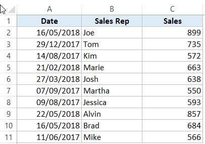
In this data set, if you have to refer to the range that has the Date, you will have to use A2:A11 in formulas. Similarly, for Sales Rep and Sales, you will have to use B2:B11 and C2:C11.
While it’s alright when you only have a couple of data points, but in case you huge complex data sets, using cell references to refer to data could be time-consuming.
Excel Named Ranges makes it easy to refer to data sets in Excel.
You can create a named range in Excel for each data category, and then use that name instead of the cell references. For example, dates can be named ‘Date’, Sales Rep data can be named ‘SalesRep’ and sales data can be named ‘Sales’.

You can also create a name for a single cell. For example, if you have the sales commission percentage in a cell, you can name that cell as ‘Commission’.
Benefits of Creating Named Ranges in Excel
Here are the benefits of using named ranges in Excel.
Use Names instead of Cell References
When you create Named Ranges in Excel, you can use these names instead of the cell references.
For example, you can use =SUM(SALES) instead of =SUM(C2:C11) for the above data set.
Have a look at ṭhe formulas listed below. Instead of using cell references, I have used the Named Ranges.
- Number of sales with value more than 500: =COUNTIF(Sales,”>500″)
- Sum of all the sales done by Tom: =SUMIF(SalesRep,”Tom”,Sales)
- Commission earned by Joe (sales by Joe multiplied by commission percentage):
=SUMIF(SalesRep,”Joe”,Sales)*Commission
You would agree that these formulas are easy to create and easy to understand (especially when you share it with someone else or revisit it yourself.
No Need to Go Back to the Dataset to Select Cells
Another significant benefit of using Named Ranges in Excel is that you don’t need to go back and select the cell ranges.
You can just type a couple of alphabets of that named range and Excel will show the matching named ranges (as shown below):

Named Ranges Make Formulas Dynamic
By using Named Ranges in Excel, you can make Excel formulas dynamic.
For example, in the case of sales commission, instead of using the value 2.5%, you can use the Named Range.
Now, if your company later decides to increase the commission to 3%, you can simply update the Named Range, and all the calculation would automatically update to reflect the new commission.
How to Create Named Ranges in Excel
Here are three ways to create Named Ranges in Excel:
Method #1 – Using Define Name
Here are the steps to create Named Ranges in Excel using Define Name:
This will create a Named Range SALESREP.
Method #2: Using the Name Box
- Select the range for which you want to create a name (do not select headers).
- Go to the Name Box on the left of Formula bar and Type the name of the with which you want to create the Named Range.

- Note that the Name created here will be available for the entire Workbook. If you wish to restrict it to a worksheet, use Method 1.
Method #3: Using Create From Selection Option
This is the recommended way when you have data in tabular form, and you want to create named range for each column/row.
For example, in the dataset below, if you want to quickly create three named ranges (Date, Sales_Rep, and Sales), then you can use the method shown below.
Here are the steps to quickly create named ranges from a dataset:
This will create three Named Ranges – Date, Sales_Rep, and Sales.
Note that it automatically picks up names from the headers. If there are any space between words, it inserts an underscore (as you can’t have spaces in named ranges).
Naming Convention for Named Ranges in Excel
There are certain naming rules you need to know while creating Named Ranges in Excel:
- The first character of a Named Range should be a letter and underscore character(_), or a backslash(). If it’s anything else, it will show an error. The remaining characters can be letters, numbers, special characters, period, or underscore.
- You can not use names that also represent cell references in Excel. For example, you can’t use AB1 as it is also a cell reference.
- You can’t use spaces while creating named ranges. For example, you can’t have Sales Rep as a named range. If you want to combine two words and create a Named Range, use an underscore, period or uppercase characters to create it. For example, you can have Sales_Rep, SalesRep, or SalesRep.
- While creating named ranges, Excel treats uppercase and lowercase the same way. For example, if you create a named range SALES, then you will not be able to create another named range such as ‘sales’ or ‘Sales’.
- A Named Range can be up to 255 characters long.
Too Many Named Ranges in Excel? Don’t Worry
Sometimes in large data sets and complex models, you may end up creating a lot of Named Ranges in Excel.
What if you don’t remember the name of the Named Range you created?
Don’t worry – here are some useful tips.
Getting the Names of All the Named Ranges
Here are the steps to get a list of all the named ranges you created:
This will give you a list of all the Named Ranges in that workbook. To use a named range (in formulas or a cell), double click on it.

Displaying the Matching Named Ranges
- If you have some idea about the Name, type a few initial characters, and Excel will show a drop down of the matching names.


How to Edit Named Ranges in Excel
If you have already created a Named Range, you can edit it using the following steps:
Useful Named Range Shortcuts (the Power of F3)
Here are some useful keyboard shortcuts that will come handy when you are working with Named Ranges in Excel:
- To get a list of all the Named Ranges and pasting it in Formula: F3
- To create new name using Name Manager Dialogue Box: Control + F3
- To create Named Ranges from Selection: Control + Shift + F3
Creating Dynamic Named Ranges in Excel
So far in this tutorial, we have created static Named Ranges.
This means that these Named Ranges would always refer to the same dataset.
For example, if A1:A10 has been named as ‘Sales’, it would always refer to A1:A10.
If you add more sales data, then you would have to manually go and update the reference in the named range.
In the world of ever-expanding data sets, this may end up taking up a lot of your time. Every time you get new data, you may have to update the Named Ranges in Excel.
To tackle this issue, we can create Dynamic Named Ranges in Excel that would automatically account for additional data and include it in the existing Named Range.
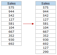
For example, For example, if I add two additional sales data points, a dynamic named range would automatically refer to A1:A12.
This kind of Dynamic Named Range can be created by using Excel INDEX function. Instead of specifying the cell references while creating the Named Range, we specify the formula. The formula automatically updated when the data is added or deleted.
Let’s see how to create Dynamic Named Ranges in Excel.
Suppose we have the sales data in cell A2:A11.

Here are the steps to create Dynamic Named Ranges in Excel:
-
- Go to the Formula tab and click on Define Name.

- In the New Name dialogue box type the following:
- Name: Sales
- Scope: Workbook
- Refers to: =$A$2:INDEX($A$2:$A$100,COUNTIF($A$2:$A$100,”<>”&””))

- Click OK.
- Go to the Formula tab and click on Define Name.


Done!
You now have a dynamic named range with the name ‘Sales’. This would automatically update whenever you add data to it or remove data from it.
How does Dynamic Named Ranges Work?
To explain how this work, you need to know a bit more about Excel INDEX function.
Most people use INDEX to return a value from a list based on the row and column number.
But the INDEX function also has another side to it.
It can be used to return a cell reference when it is used as a part of a cell reference.
For example, here is the formula that we have used to create a dynamic named range:
=$A$2:INDEX($A$2:$A$100,COUNTIF($A$2:$A$100,"<>"&""))
INDEX($A$2:$A$100,COUNTIF($A$2:$A$100,”<>”&””) –> This part of the formula is expected to return a value (which would be the 10th value from the list, considering there are ten items).
However, when used in front of a reference (=$A$2:INDEX($A$2:$A$100,COUNTIF($A$2:$A$100,”<>”&””))) it returns the reference to the cell instead of the value.
Hence, here it returns =$A$2:$A$11
If we add two additional values to the sales column, it would then return =$A$2:$A$13
When you add new data to the list, Excel COUNTIF function returns the number of non-blank cells in the data. This number is used by the INDEX function to fetch the cell reference of the last item in the list.
Note:
- This would only work if there are no blank cells in the data.
- In the example taken above, I have assigned a large number of cells (A2:A100) for the Named Range formula. You can adjust this based on your data set.
You can also use OFFSET function to create a Dynamic Named Ranges in Excel, however, since OFFSET function is volatile, it may lead a slow Excel workbook. INDEX, on the other hand, is semi-volatile, which makes it a better choice to create Dynamic Named Ranges in Excel.
You may also like the following Excel resources:
- Free Excel Templates.
- Free Online Excel Training (7-Part Online Video Course).
- Useful Excel Macro Code Examples.
- 10 Advanced Excel VLOOKUP Examples.
- Creating a Drop Down List in Excel.
- Creating a Named Range in Google Sheets.
- How to Reference Another Sheet or Workbook in Excel
- How to Delete Named Range in Excel?