Using find and if in excel - Word и Excel - помощь в работе с программами

Содержание

Excel If Cell Contains Text
If Cell Contains Text
If Cell Contains Text Then TRUE
If Cell Contains Partial Text
Find for Case Sensitive Match:
Search for Not Case Sensitive Match:
If Range of Cells Contains Text
If Cells Contains Text From List
If Cell Contains Text Then Return a Value
Excel if cell contains word then assign value
Count If Cell Contains Text
Count If Cell Contains Partial Text
If Cell contains text from list then return value
If Cell Contains Text Then SUM
Sum If Cell Contains Partial Text
VBA to check if Cell Contains Text
If Cell Contains Partial Text VBA
If Cell Contains Text Then VBA MsgBox
Which function returns true if cell a1 contains text?
Which function returns true if cell a1 contains text value?
Find and select cells that meet specific conditions
Need more help?
How To Use “If Cell Contains” Formulas in Excel
Excel Formula: If cell contains
Explanation: If Cell Contains
Using “if cell contains” formulas in Excel
1. If cell contains any value, then return a value
2. If cell contains text/number, then return a value
Check for text
Check for a number or date
3. If cell contains specific text, then return a value
4. If cell contains specific text, then return a value (case-sensitive)
5. If cell does not contain specific text, then return a value
6. If cell contains one of many text strings, then return a value
7. If cell contains several of many text strings, then return a value
Final thoughts
Before you go

Excel If Cell Contains Text

Excel If Cell Contains Text Then Formula helps you to return the output when a cell have any text or a specific text. You can check if a cell contains a some string or text and produce something in other cell. For Example you can check if a cell A1 contains text ‘example text’ and print Yes or No in Cell B1. Following are the example Formulas to check if Cell contains text then return some thing in a Cell.

If Cell Contains Text

Here are the Excel formulas to check if Cell contains specific text then return something. This will return if there is any string or any text in given Cell. We can use this simple approach to check if a cell contains text, specific text, string, any text using Excel If formula. We can use equals to operator(=) to compare the strings .

If Cell Contains Text Then TRUE

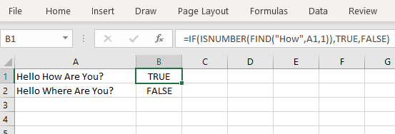
Following is the Excel formula to return True if a Cell contains Specif Text. You can check a cell if there is given string in the Cell and return True or False.

The formula will return true if it found the match, returns False of no match found.

If Cell Contains Partial Text

We can return Text If Cell Contains Partial Text. We use formula or VBA to Check Partial Text in a Cell.

Find for Case Sensitive Match:

We can check if a Cell Contains Partial Text then return something using Excel Formula. Following is a simple example to find the partial text in a given Cell. We can use if your want to make the criteria case sensitive.

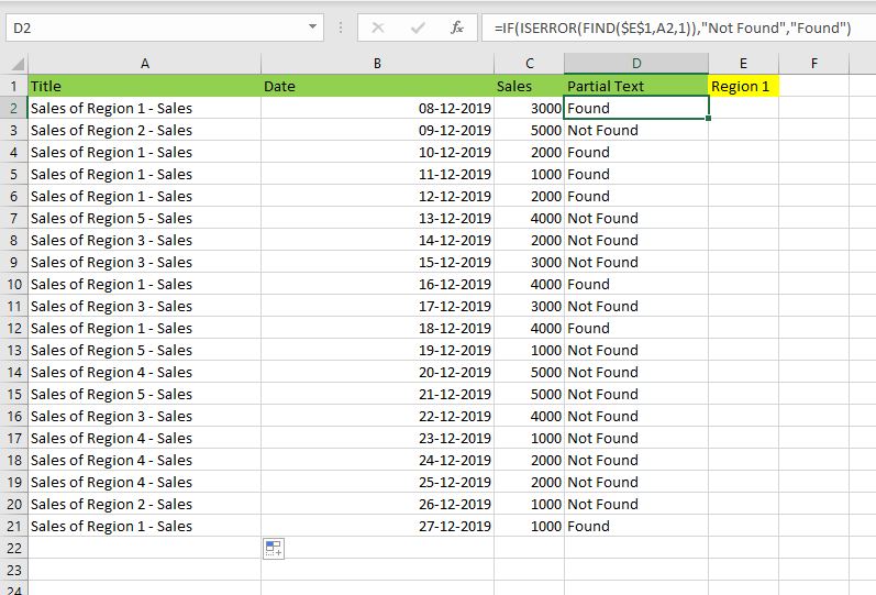
Here, Find Function returns the finding position of the given string
Use Find function is Case Sensitive
IsError Function check if Find Function returns Error, that means, string not found

Search for Not Case Sensitive Match:

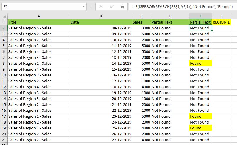
We can use Search function to check if Cell Contains Partial Text. Search function useful if you want to make the checking criteria Not Case Sensitive.

If Range of Cells Contains Text

We can check for the strings in a range of cells. Here is the formula to find If Range of Cells Contains Text. We can use Count If Formula to check the excel if range of cells contains specific text and return Text.

CountIf function counts the number of cells with given criteria
We can use If function to return the required Text
Formula displays the Text ‘Range Contains Text” if match found
Returns “Text Not Found in the Given Range” if match not found in the specified range

If Cells Contains Text From List

Below formulas returns text If Cells Contains Text from given List. You can use based on your requirement.

VlookUp to Check If Cell Contains Text from a List:
We can use VlookUp function to match the text in the Given list of Cells. And return the corresponding values.

Check if a List Contains Text:
=IF(ISERR(VLOOKUP(F1,A1:B21,2,FALSE)),”False:Not Contains”,”True: Text Found”)
Check if a List Contains Text and Return Corresponding Value:
=VLOOKUP(F1,A1:B21,2,FALSE)
Check if a List Contains Partial Text and Return its Value:
=VLOOKUP(“*”&F1&”*”,A1:B21,2,FALSE)

If Cell Contains Text Then Return a Value

We can return some value if cell contains some string. Here is the the the Excel formula to return a value if a Cell contains Text. You can check a cell if there is given string in the Cell and return some string or value in another column.

The formula will return true if it found the match, returns False of no match found. can

Excel if cell contains word then assign value

You can replace any word in the following formula to check if cell contains word then assign value.

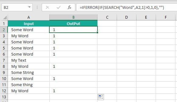
Search function will check for a given word in the required cell and return it’s position. We can use If function to check if the value is greater than 0 and assign a given value (example: 1) in the cell. search function returns #Value if there is no match found in the cell, we can handle this using IFERROR function.

Count If Cell Contains Text

We can check If Cell Contains Text Then COUNT. Here is the Excel formula to Count if a Cell contains Text. You can count the number of cells containing specific text.

The formula will Sum the values in Column B if the cells of Column A contains the given text.

Count If Cell Contains Partial Text

We can count the cells based on partial match criteria. The following Excel formula Counts if a Cell contains Partial Text.

We can use the CountIf Function to Count the Cells if they contains given String
Wild-card operators helps to make the CountIf to check for the Partial String
Put Your Text between two asterisk symbols (*YourText*) to make the criteria to find any where in the given Cell
Add Asterisk symbol at end of your text (YourText*) to make the criteria to find your text beginning of given Cell
Place Asterisk symbol at beginning of your text (*YourText) to make the criteria to find your text end of given Cell

If Cell contains text from list then return value

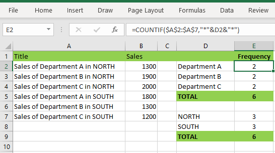
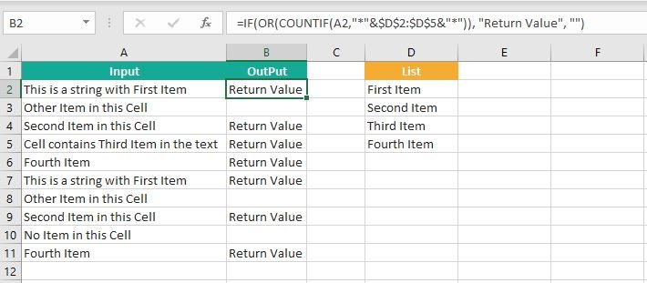
Here is the Excel Formula to check if cell contains text from list then return value. We can use COUNTIF and OR function to check the array of values in a Cell and return the given Value. Here is the formula to check the list in range D2:D5 and check in Cell A2 and return value in B2.

If Cell Contains Text Then SUM

Following is the Excel formula to Sum if a Cell contains Text. You can total the cell values if there is given string in the Cell. Here is the example to sum the column B values based on the values in another Column.

The formula will Sum the values in Column B if the cells of Column A contains the given text.

Sum If Cell Contains Partial Text

Use SumIfs function to Sum the cells based on partial match criteria. The following Excel formula Sums the Values if a Cell contains Partial Text.

SUMIFS Function will Sum the Given Sum Range
We can specify the Criteria Range, and wild-card expression to check for the Partial text
Put Your Text between two asterisk symbols (*YourText*) to Sum the Cells if the criteria to find any where in the given Cell
Add Asterisk symbol at end of your text (YourText*) to Sum the Cells if the criteria to find your text beginning of given Cell
Place Asterisk symbol at beginning of your text (*YourText) to Sum the Cells if criteria to find your text end of given Cell

VBA to check if Cell Contains Text

Here is the VBA function to find If Cells Contains Text using Excel VBA Macros.

If Cell Contains Partial Text VBA

We can use VBA to check if Cell Contains Text and Return Value. Here is the simple VBA code match the partial text. Excel VBA if Cell contains partial text macros helps you to use in your procedures and functions.

CheckIfCellContainsPartialText VBA Function returns true if Cell Contains Partial Text
inStr Function will return the Match Position in the given string

If Cell Contains Text Then VBA MsgBox

Here is the simple VBA code to display message box if cell contains text. We can use inStr Function to search for the given string. And show the required message to the user.

inStr Function will return the Match Position in the given string
blnMatch is the Boolean variable becomes True when match string
You can display the message to the user if a Range Contains Text

Which function returns true if cell a1 contains text?

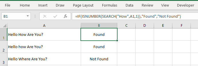
You can use the Excel If function and Find function to return TRUE if Cell A1 Contains Text. Here is the formula to return True.

Which function returns true if cell a1 contains text value?

You can use the Excel If function with Find function to return TRUE if a Cell A1 Contains Text Value. Below is the formula to return True based on the text value.

Источник

Find and select cells that meet specific conditions

Use the Go To command to quickly find and select all cells that contain specific types of data, such as formulas. Also, use Go To to find only the cells that meet specific criteria,—such as the last cell on the worksheet that contains data or formatting.

Follow these steps:

Begin by doing either of the following:

To search the entire worksheet for specific cells, click any cell.

To search for specific cells within a defined area, select the range, rows, or columns that you want. For more information, see Select cells, ranges, rows, or columns on a worksheet.

Tip: To cancel a selection of cells, click any cell on the worksheet.

On the Home tab, click Find & Select > Go To (in the Editing group).

Keyboard shortcut: Press CTRL+G.

In the Go To Special dialog box, click one of the following options.

Cells that contain comments.

Cells that contain constants.

Cells that contain formulas.

Note: The check boxes below Formulas define the type of formula.

The current region, such as an entire list.

An entire array if the active cell is contained in an array.

Graphical objects, including charts and buttons, on the worksheet and in text boxes.

All cells that differ from the active cell in a selected row. There is always one active cell in a selection—whether this is a range, row, or column. By pressing the Enter or Tab key, you can change the location of the active cell, which by default is the first cell in a row.

If more than one row is selected, the comparison is done for each individual row of that selection, and the cell that is used in the comparison for each additional row is located in the same column as the active cell.

All cells that differ from the active cell in a selected column. There is always one active cell in a selection, whether this is a range, row, or column. By pressing the Enter or Tab key, you can change the location of the active cell—which by default is the first cell in a column.

When selecting more than one column, the comparison is done for each individual column of that selection. The cell that is used in the comparison for each additional column is located in the same row as the active cell.

Cells that are referenced by the formula in the active cell. Under Dependents, do either of the following:

Click Direct only to find only cells that are directly referenced by formulas.

Click All levels to find all cells that are directly or indirectly referenced by the cells in the selection.

Cells with formulas that refer to the active cell. Do either of the following:

Click Direct only to find only cells with formulas that refer directly to the active cell.

Click All levels to find all cells that directly or indirectly refer to the active cell.

The last cell on the worksheet that contains data or formatting.

Visible cells only

Only cells that are visible in a range that crosses hidden rows or columns.

Only cells that have conditional formats applied. Under Data validation, do either of the following:

Click All to find all cells that have conditional formats applied.

Click Same to find cells that have the same conditional formats as the currently selected cell.

Only cells that have data validation rules applied. Do either of the following:

Click All to find all cells that have data validation applied.

Click Same to find cells that have the same data validation as the currently selected cell.

Need more help?

You can always ask an expert in the Excel Tech Community or get support in the Answers community.

Источник

How To Use “If Cell Contains” Formulas in Excel

Excel has a number of formulas that help you use your data in useful ways. For example, you can get an output based on whether or not a cell meets certain specifications. Right now, we’ll focus on a function called “if cell contains, then”. Let’s look at an example.

Excel Formula: If cell contains

To test for cells that contain certain text, you can use a formula that uses the IF function together with the SEARCH and ISNUMBER functions. In the example shown, the formula in C5 is:

If you want to check whether or not the A1 cell contains the text “Example”, you can run a formula that will output “Yes” or “No” in the B1 cell. There are a number of different ways you can put these formulas to use. At the time of writing, Excel is able to return the following variations:

If cell contains any value
If cell contains text
If cell contains number
If cell contains specific text
If cell contains certain text string
If cell contains one of many text strings
If cell contains several strings

Using these scenarios, you’re able to check if a cell contains text, value, and more.

Explanation: If Cell Contains

One limitation of the IF function is that it does not support Excel wildcards like «?» and «*». This simply means you can’t use IF by itself to test for text that may appear anywhere in a cell.

One solution is a formula that uses the IF function together with the SEARCH and ISNUMBER functions. For example, if you have a list of email addresses, and want to extract those that contain «ABC», the formula to use is this:

If «abc» is found anywhere in a cell B5, IF will return that value. If not, IF will return an empty string («»). This formula’s logical test is this bit:

Using “if cell contains” formulas in Excel

The guides below were written using the latest Microsoft Excel 2019 for Windows 10 . Some steps may vary if you’re using a different version or platform. Contact our experts if you need any further assistance.

1. If cell contains any value, then return a value

This scenario allows you to return values based on whether or not a cell contains any value at all. For example, we’ll be checking whether or not the A1 cell is blank or not, and then return a value depending on the result.

Select the output cell, and use the following formula: =IF(cell<>«», value_to_return, «») .
For our example, the cell we want to check is A2 , and the return value will be No . In this scenario, you’d change the formula to =IF(A2<>«», «No», «») .

Since the A2 cell isn’t blank, the formula will return “ No ” in the output cell. If the cell you’re checking is blank, the output cell will also remain blank.

2. If cell contains text/number, then return a value

With the formula below, you can return a specific value if the target cell contains any text or number. The formula will ignore the opposite data types.

Check for text

To check if a cell contains text, select the output cell, and use the following formula: =IF(ISTEXT(cell), value_to_return, «») .
For our example, the cell we want to check is A2 , and the return value will be Yes . In this scenario, you’d change the formula to =IF(ISTEXT(A2), «Yes», «») .
Because the A2 cell does contain text and not a number or date, the formula will return “ Yes ” into the output cell.

Check for a number or date

To check if a cell contains a number or date, select the output cell, and use the following formula: =IF(ISNUMBER(cell), value_to_return, «») .
For our example, the cell we want to check is D2 , and the return value will be Yes . In this scenario, you’d change the formula to =IF(ISNUMBER(D2), «Yes», «») .
Because the D2 cell does contain a number and not text, the formula will return “ Yes ” into the output cell.

3. If cell contains specific text, then return a value

To find a cell that contains specific text, use the formula below.

Select the output cell, and use the following formula: =IF(cell=»text», value_to_return, «») .
For our example, the cell we want to check is A2 , the text we’re looking for is “ example ”, and the return value will be Yes . In this scenario, you’d change the formula to =IF(A2=»example», «Yes», «») .
Because the A2 cell does consist of the text “ example ”, the formula will return “ Yes ” into the output cell.

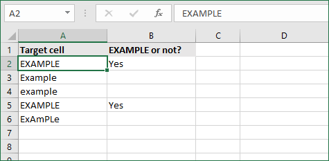
4. If cell contains specific text, then return a value (case-sensitive)

To find a cell that contains specific text, use the formula below. This version is case-sensitive, meaning that only cells with an exact match will return the specified value.

Select the output cell, and use the following formula: =IF(EXACT(cell,»case_sensitive_text»), «value_to_return», «») .
For our example, the cell we want to check is A2 , the text we’re looking for is “ EXAMPLE ”, and the return value will be Yes . In this scenario, you’d change the formula to =IF(EXACT(A2,»EXAMPLE»), «Yes», «») .
Because the A2 cell does consist of the text “ EXAMPLE ” with the matching case, the formula will return “ Yes ” into the output cell.

5. If cell does not contain specific text, then return a value

The opposite version of the previous section. If you want to find cells that don’t contain a specific text, use this formula.

Select the output cell, and use the following formula: =IF(cell=»text», «», «value_to_return») .
For our example, the cell we want to check is A2 , the text we’re looking for is “ example ”, and the return value will be No . In this scenario, you’d change the formula to =IF(A2=»example», «», «No») .
Because the A2 cell does consist of the text “ example ”, the formula will return a blank cell. On the other hand, other cells return “ No ” into the output cell.

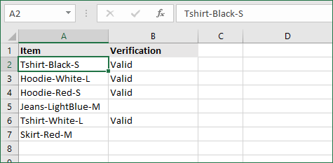
6. If cell contains one of many text strings, then return a value

This formula should be used if you’re looking to identify cells that contain at least one of many words you’re searching for.

Select the output cell, and use the following formula: =IF(OR(ISNUMBER(SEARCH(«string1», cell)), ISNUMBER(SEARCH(«string2», cell))), value_to_return, «») .
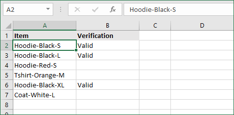
For our example, the cell we want to check is A2 . We’re looking for either “ tshirt ” or “ hoodie ”, and the return value will be Valid . In this scenario, you’d change the formula to =IF(OR(ISNUMBER(SEARCH(«tshirt»,A2)),ISNUMBER(SEARCH(«hoodie»,A2))),»Valid «,»») .
Because the A2 cell does contain one of the text values we searched for, the formula will return “ Valid ” into the output cell.

To extend the formula to more search terms, simply modify it by adding more strings using ISNUMBER(SEARCH(«string», cell)) .

7. If cell contains several of many text strings, then return a value

This formula should be used if you’re looking to identify cells that contain several of the many words you’re searching for. For example, if you’re searching for two terms, the cell needs to contain both of them in order to be validated.

Select the output cell, and use the following formula: =IF(AND(ISNUMBER(SEARCH(«string1»,cell)), ISNUMBER(SEARCH(«string2″,cell))), value_to_return,»») .
For our example, the cell we want to check is A2 . We’re looking for “ hoodie ” and “ black ”, and the return value will be Valid . In this scenario, you’d change the formula to =IF(AND(ISNUMBER(SEARCH(«hoodie»,A2)),ISNUMBER(SEARCH(«black»,A2))),»Valid «,»») .
Because the A2 cell does contain both of the text values we searched for, the formula will return “ Valid ” to the output cell.

Final thoughts

We hope this article was useful to you in learning how to use “if cell contains” formulas in Microsoft Excel. Now, you can check if any cells contain values, text, numbers, and more. This allows you to navigate, manipulate and analyze your data efficiently.

We’re glad you’re read the article up to here 🙂 Thank you 🙂

Please share it on your socials. Someone else will benefit.

Before you go

If you need any further help with Excel, don’t hesitate to reach out to our customer service team, which is available 24/7 to assist you. Return to us for more informative articles all related to productivity and modern-day technology!

Would you like to receive promotions, deals, and discounts to get our products for the best price? Don’t forget to subscribe to our newsletter by entering your email address below! Receive the latest technology news in your inbox and be the first to read our tips to become more productive.

Источник

Excel If Cell Contains Text

If Cell Contains Text

If Cell Contains Text Then TRUE

Following is the Excel formula to return True if a Cell contains Specif Text. You can check a cell if there is given string in the Cell and return True or False.

=IF(ISNUMBER(FIND(“How”,A1,1)),TRUE,FALSE)

The formula will return true if it found the match, returns False of no match found.

If Cell Contains Partial Text

We can return Text If Cell Contains Partial Text. We use formula or VBA to Check Partial Text in a Cell.

Find for Case Sensitive Match:

=IF(ISERROR(FIND($E$1,A2,1)),”Not Found”,”Found”)

Here, Find Function returns the finding position of the given string
Use Find function is Case Sensitive
IsError Function check if Find Function returns Error, that means, string not found

Search for Not Case Sensitive Match:

We can use Search function to check if Cell Contains Partial Text. Search function useful if you want to make the checking criteria Not Case Sensitive.

=IF(ISERROR(SEARCH($F$1,A2,1)),”Not Found”,”Found”)

If Range of Cells Contains Text

=IF(COUNTIF(A2:A21, “*Region 1d*”)>0,”Range Contais Text”,”Text Not Found in the Given Range”)

CountIf function counts the number of cells with given criteria
We can use If function to return the required Text
Formula displays the Text ‘Range Contains Text” if match found
Returns “Text Not Found in the Given Range” if match not found in the specified range

If Cells Contains Text From List

Below formulas returns text If Cells Contains Text from given List. You can use based on your requirement.

VlookUp to Check If Cell Contains Text from a List:
We can use VlookUp function to match the text in the Given list of Cells. And return the corresponding values.

Check if a List Contains Text:
=IF(ISERR(VLOOKUP(F1,A1:B21,2,FALSE)),”False:Not Contains”,”True: Text Found”)
Check if a List Contains Text and Return Corresponding Value:
=VLOOKUP(F1,A1:B21,2,FALSE)
Check if a List Contains Partial Text and Return its Value:
=VLOOKUP(“*”&F1&”*”,A1:B21,2,FALSE)

If Cell Contains Text Then Return a Value

=IF(ISNUMBER(SEARCH(“How”,A1,1)),”Found”,”Not Found”)

The formula will return true if it found the match, returns False of no match found. can

Excel if cell contains word then assign value

You can replace any word in the following formula to check if cell contains word then assign value.

=IFERROR(IF(SEARCH(“Word”,A2,1)>0,1,0),””)

Count If Cell Contains Text

We can check If Cell Contains Text Then COUNT. Here is the Excel formula to Count if a Cell contains Text. You can count the number of cells containing specific text.

=COUNTIF($A$2:$A$7,”*”&D2&”*”)

The formula will Sum the values in Column B if the cells of Column A contains the given text.

Count If Cell Contains Partial Text

We can count the cells based on partial match criteria. The following Excel formula Counts if a Cell contains Partial Text.

=COUNTIF(A2:A21, “*Region 1*”)

We can use the CountIf Function to Count the Cells if they contains given String
Wild-card operators helps to make the CountIf to check for the Partial String
Put Your Text between two asterisk symbols (*YourText*) to make the criteria to find any where in the given Cell
Add Asterisk symbol at end of your text (YourText*) to make the criteria to find your text beginning of given Cell
Place Asterisk symbol at beginning of your text (*YourText) to make the criteria to find your text end of given Cell

If Cell contains text from list then return value

=IF(OR(COUNTIF(A2,”*”&$D$2:$D$5&”*”)), “Return Value”, “”)

If Cell Contains Text Then SUM

=SUMIF($A$2:$A$7,”*”&D2&”*”,$B$2:$B$7)

The formula will Sum the values in Column B if the cells of Column A contains the given text.

Sum If Cell Contains Partial Text

Use SumIfs function to Sum the cells based on partial match criteria. The following Excel formula Sums the Values if a Cell contains Partial Text.

=SUMIFS(C2:C21,A2:A21, “*Region 1*”)

SUMIFS Function will Sum the Given Sum Range
We can specify the Criteria Range, and wild-card expression to check for the Partial text
Put Your Text between two asterisk symbols (*YourText*) to Sum the Cells if the criteria to find any where in the given Cell
Add Asterisk symbol at end of your text (YourText*) to Sum the Cells if the criteria to find your text beginning of given Cell
Place Asterisk symbol at beginning of your text (*YourText) to Sum the Cells if criteria to find your text end of given Cell

VBA to check if Cell Contains Text

Here is the VBA function to find If Cells Contains Text using Excel VBA Macros.

If Cell Contains Partial Text VBA

Sub sbCkeckforPartialText()
MsgBox CheckIfCellContainsPartialText(Cells(2, 1), “Region 1”)
End Sub
Function CheckIfCellContainsPartialText(ByVal cell As Range, ByVal strText As String) As Boolean
If InStr(1, cell.Value, strText) > 0 Then CheckIfCellContainsPartialText = True
End Function

CheckIfCellContainsPartialText VBA Function returns true if Cell Contains Partial Text
inStr Function will return the Match Position in the given string

If Cell Contains Text Then VBA MsgBox

Here is the simple VBA code to display message box if cell contains text. We can use inStr Function to search for the given string. And show the required message to the user.

Sub sbVBAIfCellsContainsText()
If InStr(1, Cells(2, 1), “Region 3”) > 0 Then blnMatch = True
If blnMatch = True Then MsgBox “Cell Contains Text”
End Sub

inStr Function will return the Match Position in the given string
blnMatch is the Boolean variable becomes True when match string
You can display the message to the user if a Range Contains Text

Which function returns true if cell a1 contains text?

You can use the Excel If function and Find function to return TRUE if Cell A1 Contains Text. Here is the formula to return True.

=IF(ISNUMBER(FIND(“YourText”,A1,1)),TRUE,FALSE)

Which function returns true if cell a1 contains text value?

You can use the Excel If function with Find function to return TRUE if a Cell A1 Contains Text Value. Below is the formula to return True based on the text value.

=IF(ISNUMBER(FIND(“YourTextValue”,A1,1)),TRUE,FALSE)

Share This Story, Choose Your Platform!

7 Comments

Meghana
December 27, 2019 at 1:42 pm — Reply

Hi Sir,Thank you for the great explanation, covers everything and helps use create formulas if cell contains text values.

Many thanks! Meghana!!
Max
December 27, 2019 at 4:44 pm — Reply

Perfect! Very Simple and Clear explanation. Thanks!!
Mike Song
August 29, 2022 at 2:45 pm — Reply

I tried this exact formula and it did not work.
Theresa A Harding
October 18, 2022 at 9:51 pm — Reply
Marko
November 3, 2022 at 9:21 pm — Reply

Hi

Is possible to sum all WA11?

(A1) WA11 4

(A2) AdBlue 1, WA11 223

(A3) AdBlue 3, WA11 32, shift 4

… and everything is in one column.

Thanks you very much for your help.

Sincerely Marko
Mike
December 9, 2022 at 9:59 pm — Reply

Thank you for the help. The formula =OR(COUNTIF(M40,”*”&Vendors&”*”)) will give “TRUE” when some part of M40 contains a vendor from “Vendors” list. But how do I get Excel to tell which vendor it found in the M40 cell?
- PNRao
  December 18, 2022 at 6:05 am — Reply
  
  Please describe your question more elaborately.
  Thanks!

Page load link

Источник

I have an excel document I have to process regularly, while awaiting my company to build an automated process for this, and the issue we recently found is that the formula I’m using strips can’t return a result other than #VALUE! when the FIND formula fails to find the text I need it to.

the formula we currently have is:

=IF(FIND("-",M2,3),RIGHT(M2,2))

The cells this formula checks have states, & provinces in them which look like so «CA-ON» or «US-NV».
The problem is that regions for the UK don’t fillout as «UK-XX» it inputs the actual county for example «Essex» or «Merryside»

What I need the formula to do is, if it can’t find the hyphen(-) in the cell, then it should just take whatever value is there and write it in the cell the formula is in.

I should also mention that some of the cells are also blank, since this is an optional field. Is there anyway to run this formula where if it doesn’t find the «-» it just writes whats there?

Источник

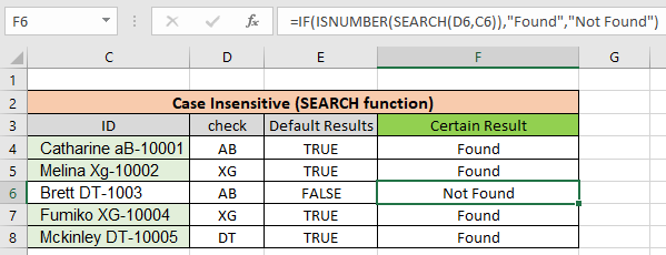
In this article, we will learn How to look up cells having certain text and return the Certain Text in Excel.

Scenario :

Identify particular text in a cell or different word in given cells. For example finding the department ID from a database. I think you must have thought to do it manually but time constraint. You are here at the right place to learn How to check if a cell contains specific text.

Generic formula:

The text you are looking for can either be exact or case insensitive. Case insensitive means formula looks for AG can return ag, Ag, AG or aG.

Case insensitive formula:

=ISNUMBER(SEARCH(find_text,within_text)

find_text : text to find

within_text : to find in text

Case sensitive formula:

=ISNUMBER(FIND(find_text,within_text)

find_text : text to find

within_text : to find in text

Note:

The above formulas will return True or False. Use the IF function with formula to return YES or NO. Use the below formula to get the certain required result format.

Case insensitive formula:

=IF(ISNUMBER(SEARCH(find_text,within_text)),»value_if_true»,value_if_false)

find_text : text to find

within_text : to find in text

Case sensitive formula:

=IF(ISNUMBER(FIND(find_text,within_text)),»value_if_true»,value_if_false)

find_text : text to find

within_text : to find in text

Note: In The above mentioned formula you can input values like YES/NO or Found/Notfound.

Example :

All of these might be confusing to understand. Let’s understand how to use the function using an example. Here we have some employees to look up by the given department Id. Employee id has name, department id and particular id. Here lookup text is in column D and within text is in Column C.

Use the formula:

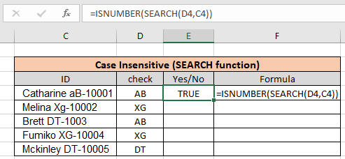
As you can see the formula finds AB when you looked for

AB using the Search function. Copy the formula to the rest of the cells using the Ctrl + D or dragging it down from the right bottom (tiny box) of the applied cell.

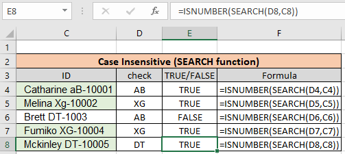
As you can see we found all the given department id employees using the above method. Now we will check if all cells contain specific text.

Another Example: (Case Sensitive)

Here we have been given a list of Employee Id information in column A and the look up department is «XG». Here we need to find the department «XG» in all cells. «XG» must be exact as there are two different departments that go by «Xg». So check only «XG» in all cells and return «Yes» if found and return «No» If not.

Use the formula:

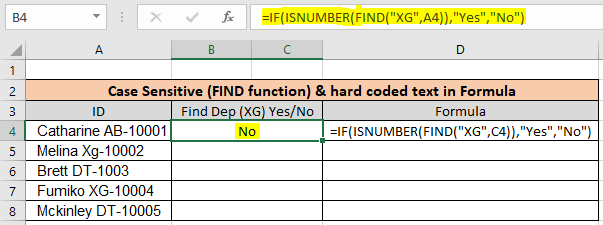
As you can see First employee doesn’t belong to «XG» so the formula returns «No» using the FIND function. Copy the formula to the rest of the cells using the Ctrl + D or dragging it down from the right bottom (tiny box) of the applied cell.

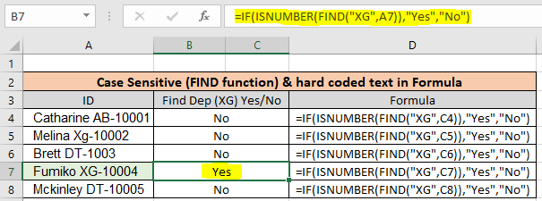
As you can see there is only one employee in «XG» department. This formula is useful wherever the database contains multiple information of a row in one cell.

Check if cell Matches multiple text

In the above example we lookup one given text in cells. If we have multiple texts then we use the SUMPRODUCT function, This formula returns TRUE/FALSE as per the value found/ Not found.

Use the formula:

=SUMPRODUCT(—ISNUMBER(SEARCH(,A1)))>0

Learn more about this formula. Follow this link How to Check if a string contains one of many texts in Excel.

Here are all the observational notes using the above explained formulas in Excel
Notes :

Use the «find_text» in quotes when using hard coded values. Or else use cell reference as explained in the first example.
SEARCH is case insensitive function whereas FIND is the case Sensitive dunction.
Use the IF function, if you want to get the result in required forms like YES/NO or Found/Notfound.

Hope this article about How to lookup cells having certain text and returns the Certain Text in Excel is explanatory. Find more articles on calculating values and related Excel formulas here. If you liked our blogs, share it with your friends on Facebook. And also you can follow us on Twitter and Facebook. We would love to hear from you, do let us know how we can improve, complement or innovate our work and make it better for you. Write to us at info@exceltip.com.

Related Articles :

Searching a String for a Specific Substring in Excel : Find cells if cell contains given word in Excel using the FIND or SEARCH function.

Highlight cells that contain specific text : Highlight cells if cell contains given word in Excel using the formula under Conditional formatting

How to Check if a string contains one of many texts in Excel : lookup cells if cell contains from given multiple words in Excel using the FIND or SEARCH function.

Count Cells that contain specific text : Count number of cells if cell contains given text using one formula in Excel.

How to lookup cells having certain text and returns the Certain Text in Excel : find cells if cell contains certain text and returns required results using the IF function in Excel.

Popular Articles :

How to use the IF Function in Excel : The IF statement in Excel checks the condition and returns a specific value if the condition is TRUE or returns another specific value if FALSE.

How to use the VLOOKUP Function in Excel : This is one of the most used and popular functions of excel that is used to lookup value from different ranges and sheets.

How to use the SUMIF Function in Excel : This is another dashboard essential function. This helps you sum up values on specific conditions.

How to use the COUNTIF Function in Excel : Count values with conditions using this amazing function. You don’t need to filter your data to count specific values. Countif function is essential to prepare your dashboard.

Источник

If you use Excel often, you’re already aware of its numerous useful functions. Many of these formulas perform calculations or analyze data. However, if you want to make life easier when working with large data sets, you should know about the FIND function. What is the syntactical structure? How do you use the function? And what’s the difference between FIND and FINDB? You can find this out and more in the following article.

Contents

What is the Excel FIND formula used for?
Excel FIND function – the syntax explained
The Excel FIND function in practice
1. FIND & FIND: Nested groups
2. FIND & ISNUMBER: True or false statements
3. FIND & MID: Extracting characters
4. FIND & IF: If, then, otherwise
5. FIND & IF: If, then, otherwise

Build your brand on a great domain, including SSL and a personal consultant!

Private registration

24/7 support

Email

What is the Excel FIND formula used for?

It’s easy to lose track of things when working in large spreadsheets with hundreds of rows. Like all other Office products, Excel has a built-in search function. But that isn’t always what you actually need. The search function automatically searches the entire document, meaning you can’t narrow down the range. More importantly, you can’t use the returned values in other functions. You can’t forward the search result because the search function operates only on the interface.

But if you want to search within specific cells and integrate the search directly into your worksheet, you can use the FIND function. Simply enter the word or phrase and the function to find the location of the first occurrence of your search term in the text string (meaning the text in the cell).

The FIND function in Excel is a building block with a range of further applications. Combine FIND with other functions to unlock its full potential. For example, you can use it to see whether a certain term appears in your worksheet or to extract specific parts of a text string.

Tip

You can also use VLOOKUP as an alternative search function in Excel.

Excel FIND function – the syntax explained

The syntax of FIND isn’t very complex. In the standard version, you only have to specify two arguments: What do you want to find? And where do you want to find it?

You can also customize your search to start at a specific character:

You can use the parameters to specify various information:

Find_text: This is the text string you want to find. You have to enclose the text in quotes. You can also specify the cell containing the text. This parameter is always case-sensitive.
Within_text: This parameter specifies the text within which you want to search. You typically specify a cell containing the text. You could also type the text directly into the formula. In that case, you also have to enclose it in quotes.
Start_num: You use a numerical value to specify the character where the search is to start. This parameter is optional. If you don’t enter this value, the search will start at position 1.

Note

The FIND function is case-sensitive and does not support wildcards. To get around this restriction, you can use the SEARCH function.

Excel returns a number as the result. This value tells you where the search string begins, meaning the first occurrence from left to right. If the term occurs again in the cell, the FIND function will disregard it by itself. To find further positions, you have to use nesting. The returned value counts every single character, including spaces. The number indicates the position of the first character of the returned string. This means that the first letter or number of the search is counted in the result.

Besides FIND, Excel also offers the FINDB function. Both functions achieve the same results and have identical syntax. They only differ in the character sets they support. FIND only works with single-byte character sets (SBCS). This includes the Latin alphabet. If you use Asian characters from Chinese, Japanese and Korean (CJK), use FINDB because it supports double-byte character sets (DBCS) for these languages. Each character is encoded in two bytes, so counting is adjusted accordingly.

Tip

To work faster in Excel, you should learn the most important Excel shortcuts.

The Excel FIND function in practice

For many users, the purpose of this function is not always immediately apparent. Finding the position of a search term within a text doesn’t seem all that useful at first. But the true power of this function is revealed when used in combination with other functions.

FIND & FIND: Nested groups

Suppose we want to find the second, third or nth occurrence of the search term rather than the first.

=FIND(Searchtext;Text;FIND(Searchtext;Text)+1)

This formula shows how you can use the optional third parameter. In the start_num position of this formula, we once again insert the formula that returns the position of the first occurrence. This value plus one indicates the position at which you want the search to begin. If you then want to find a third position, nest the function again, and so on.

FIND & ISNUMBER: True or false statements

The FIND function in Excel allows you to form a true or false statement from the specified position: Does the text contain the search term or not?

=ISNUMBER(FIND("Teddybear";B2))

The ISNUMBER function returns the value TRUE if the result of FIND is a number, otherwise it will return FALSE. Since the FIND function in Excel specifies the position of the term as a whole number, the ISNUMBER function can respond to it. If the text does not contain the search term, FIND returns an error message, which of course is not a number, and ISNUMBER responds accordingly with FALSE.

You may also be interested in seeing where search terms appear. You can do this if you’ve entered data in multiple cells, such as a list of products sold. You can add this formula (like any other formula) to the conditional formatting rules. This allows you to select any sales entry related to teddy bears, for example.

Conditional formatting in Excel with FIND function

You can have Excel display specific cells by combining the FIND function with the ISNUMBER function.

FIND & MID: Extracting characters

Product codes can be very long and confusing, so you may want to extract a certain number of characters from a string. Excel provides three functions for this purpose: LEFT, RIGHT and MID. These are very useful on their own, but the formulas are even more powerful when combined with FIND. Suppose your product codes always follow a specific pattern consisting of letters, numbers, and hyphens: ABCDE-A-12345-T. You want to extract the numerical part in the middle.

However, because the string does not have a fixed length, you can’t use the basic extract functions. These functions require a specific number of characters, which you can’t easily provide in this case. But thanks to the hyphens, you can use the FIND function. It gives you the position information you need.

Since there are multiple hyphens in the string, you have to nest the FIND function. In this example, we’re assuming that the number part always contains five characters.

FIND & IF: If, then, otherwise

Since there are multiple hyphens in the string, you have to nest the FIND function. In this example, we’re assuming that the number part always contains five characters.

=PART(A2;FIND("-"; A2;FIND("-"; A2;FIND("-";A2)+1))+1;5)

The FIND function in Excel can help you extract a specific number of characters from a cell.

However, if the length is not defined, further nesting of FIND functions can be helpful. Since the string you want to find ends in a hyphen, you can search for it to determine the length.

=PART(A2;FIND("-";A2;FIND("-";A2;FIND("-";A2)+1))+1; FIND("-";A2;FIND("-";A2;FIND("-";A2)+1)+1)-FIND("-";A2;FIND("-";A2;FIND("-";A2)-1))-3)

Admittedly, this formula is very confusing, but it actually manages to achieve the goal. No matter how many characters you place between the two hyphens, Excel will always extract the correct characters using the FIND function.

Worksheet in Excel with FIND and MID function

Highly nested, but effective: This is how you extract the exact range you want.

FIND & IF: If, then, otherwise

You can also easily combine FIND with IF. For example, you may want a certain action to happen if a specific string occurs in the cell. You can do this by combining IF and FIND: If the string appears, this will happen, otherwise that will happen. A problem may arise if FIND returns an error if the string does not appear. Therefore, you also have to use the ISERROR function.

=IF(ISNUMBER(MATCH(B2,A:A,0)),1,0)

If the FIND function doesn’t find the search term (“bear” in this example), it returns an error message. For ISERROR, this means the condition is met and IF returns the first option: No, the search term does not appear. However, if the FIND function finds the string, it returns a number, which does not meet the condition for ISERROR. The alternative is returned: Yes, the search term appears.

Worksheet in Excel with FIND function and IF function

You can combine FIND, IF and ISERROR to find parts of words.

Summary

FIND is a helpful function, especially when combined with other functions. It has a wide range of combination options and different applications. This small but useful function can help you solve many problems you encounter when creating formulas in Excel.

HiDrive Cloud Storage with IONOS!

Based in Europe, HiDrive secures your data in the cloud so you can easily access it from any device!

Highly secure

Shared access

Available anywhere

Related articles

Faster with Excel: the VLOOKUP function explained

It can often be incredibly time-consuming to search for a specific entry in an Excel table by hand, which is where VLOOKUP comes into play. This practical function allows you to find the exact value for a specific search criterion. The VLOOKUP function is indispensable for managing price lists, members directories, and inventory catalogues. To ensure you can benefit from this practical function,…

Faster with Excel: the VLOOKUP function explained

Excel if-then: how the IF function works

Excel’s if-then statement is one of its most helpful formulas. In many situations, you can create a logical comparison: if A is true, then B, otherwise C. To use this useful if-then formula in Excel, you first need to understand how it works and precisely how to use it. For example, which syntax rules does the IF function follow, and how can you extend the formula?

Excel if-then: how the IF function works

Using IFERROR function in Excel to avoid problems

Error messages are never fun. That’s why Excel has the IFERROR function. It allows you to catch error messages and replace them with a custom message or a value. Most importantly, the helpful IFERROR function ensures that your whole formula doesn’t fall apart if you make a typo.

Using IFERROR function in Excel to avoid problems

The Excel SUMIF function explained

Get more out of Excel: SUMIF makes it easier to work with balance sheets and analyses. Add only the values you need – completely automatically. From simple calculations to complex formulas, it’s all possible with the SUMIF function in Excel. How do you use the function? And what does the syntax look like?

The Excel SUMIF function explained

Excel SEARCH: tips for using the Excel SEARCH function

The SEARCH function in Excel gives you the ability to quickly perform complex analyses of large data sets, clean up your data, and stay on top of your documents. When used correctly, the Excel SEARCH function is a highly effective tool. In this overview, you’ll learn more about how to use this convenient feature.

Excel SEARCH: tips for using the Excel SEARCH function

Источник

Excel for Microsoft 365 Excel 2021 Excel 2019 Excel 2016 Excel 2013 Excel 2010 Excel 2007 Access 2007 More…Less

Use the Go To command to quickly find and select all cells that contain specific types of data, such as formulas. Also, use Go To to find only the cells that meet specific criteria,—such as the last cell on the worksheet that contains data or formatting.

Follow these steps:

Begin by doing either of the following:
- To search the entire worksheet for specific cells, click any cell.
- To search for specific cells within a defined area, select the range, rows, or columns that you want. For more information, see Select cells, ranges, rows, or columns on a worksheet.
  
  Tip: To cancel a selection of cells, click any cell on the worksheet.
On the Home tab, click Find & Select > Go To (in the Editing group).

Keyboard shortcut: Press CTRL+G.
Click Special.
In the Go To Special dialog box, click one of the following options.

Click	To select
Comments	Cells that contain comments.
Constants	Cells that contain constants.
Formulas	Cells that contain formulas. Note: The check boxes below Formulas define the type of formula.
Blanks	Blank cells.
Current region	The current region, such as an entire list.
Current array	An entire array if the active cell is contained in an array.
Objects	Graphical objects, including charts and buttons, on the worksheet and in text boxes.
Row differences	All cells that differ from the active cell in a selected row. There is always one active cell in a selection—whether this is a range, row, or column. By pressing the Enter or Tab key, you can change the location of the active cell, which by default is the first cell in a row. If more than one row is selected, the comparison is done for each individual row of that selection, and the cell that is used in the comparison for each additional row is located in the same column as the active cell.
Column differences	All cells that differ from the active cell in a selected column. There is always one active cell in a selection, whether this is a range, row, or column. By pressing the Enter or Tab key, you can change the location of the active cell—which by default is the first cell in a column. When selecting more than one column, the comparison is done for each individual column of that selection. The cell that is used in the comparison for each additional column is located in the same row as the active cell.
Precedents	Cells that are referenced by the formula in the active cell. Under Dependents, do either of the following: Click Direct only to find only cells that are directly referenced by formulas. Click All levels to find all cells that are directly or indirectly referenced by the cells in the selection.
Dependents	Cells with formulas that refer to the active cell. Do either of the following: Click Direct only to find only cells with formulas that refer directly to the active cell. Click All levels to find all cells that directly or indirectly refer to the active cell.
Last cell	The last cell on the worksheet that contains data or formatting.
Visible cells only	Only cells that are visible in a range that crosses hidden rows or columns.
Conditional formats	Only cells that have conditional formats applied. Under Data validation, do either of the following: Click All to find all cells that have conditional formats applied. Click Same to find cells that have the same conditional formats as the currently selected cell.
Data validation	Only cells that have data validation rules applied. Do either of the following: Click All to find all cells that have data validation applied. Click Same to find cells that have the same data validation as the currently selected cell.

Need more help?

You can always ask an expert in the Excel Tech Community or get support in the Answers community.

Need more help?

Want more options?

Explore subscription benefits, browse training courses, learn how to secure your device, and more.

Communities help you ask and answer questions, give feedback, and hear from experts with rich knowledge.

Источник

Jump To Specific Section:

Explanation: If Cell Contains
If cell contains any value, then return a value
If cell contains text/number, then return a value
If cell contains specific text, then return a value
If cell contains specific text, then return a value (case-sensitive)
If cell does not contain specific text, then return a value
If cell contains one of many text strings, then return a value
If cell contains several of many text strings, then return a value

Excel Formula: If cell contains

Generic formula

=IF(ISNUMBER(SEARCH("abc",A1)),A1,"")

Summary

To test for cells that contain certain text, you can use a formula that uses the IF function together with the SEARCH and ISNUMBER functions. In the example shown, the formula in C5 is:

=IF(ISNUMBER(SEARCH("abc",B5)),B5,"")

If cell contains any value
If cell contains text
If cell contains number
If cell contains specific text
If cell contains certain text string
If cell contains one of many text strings
If cell contains several strings

Using these scenarios, you’re able to check if a cell contains text, value, and more.

Explanation: If Cell Contains

One limitation of the IF function is that it does not support Excel wildcards like «?» and «*». This simply means you can’t use IF by itself to test for text that may appear anywhere in a cell.

=IF(ISNUMBER(SEARCH("abc",B5)),B5,""). Assuming cells run to B5

If «abc» is found anywhere in a cell B5, IF will return that value. If not, IF will return an empty string («»). This formula’s logical test is this bit:

ISNUMBER(SEARCH("abc",B5))

Read article: Excel efficiency: 11 Excel Formulas To Increase Your Productivity

Using “if cell contains” formulas in Excel

The guides below were written using the latest Microsoft Excel 2019 for Windows 10. Some steps may vary if you’re using a different version or platform. Contact our experts if you need any further assistance.

1. If cell contains any value, then return a value

Select the output cell, and use the following formula: =IF(cell<>»», value_to_return, «»).
For our example, the cell we want to check is A2, and the return value will be No. In this scenario, you’d change the formula to =IF(A2<>»», «No», «»).
Since the A2 cell isn’t blank, the formula will return “No” in the output cell. If the cell you’re checking is blank, the output cell will also remain blank.

2. If cell contains text/number, then return a value

With the formula below, you can return a specific value if the target cell contains any text or number. The formula will ignore the opposite data types.

Check for text

To check if a cell contains text, select the output cell, and use the following formula: =IF(ISTEXT(cell), value_to_return, «»).
For our example, the cell we want to check is A2, and the return value will be Yes. In this scenario, you’d change the formula to =IF(ISTEXT(A2), «Yes», «»).
Because the A2 cell does contain text and not a number or date, the formula will return “Yes” into the output cell.

Check for a number or date

To check if a cell contains a number or date, select the output cell, and use the following formula: =IF(ISNUMBER(cell), value_to_return, «»).
For our example, the cell we want to check is D2, and the return value will be Yes. In this scenario, you’d change the formula to =IF(ISNUMBER(D2), «Yes», «»).
Because the D2 cell does contain a number and not text, the formula will return “Yes” into the output cell.

3. If cell contains specific text, then return a value

To find a cell that contains specific text, use the formula below.

Select the output cell, and use the following formula: =IF(cell=»text», value_to_return, «»).
For our example, the cell we want to check is A2, the text we’re looking for is “example”, and the return value will be Yes. In this scenario, you’d change the formula to =IF(A2=»example», «Yes», «»).
Because the A2 cell does consist of the text “example”, the formula will return “Yes” into the output cell.

4. If cell contains specific text, then return a value (case-sensitive)

To find a cell that contains specific text, use the formula below. This version is case-sensitive, meaning that only cells with an exact match will return the specified value.

Select the output cell, and use the following formula: =IF(EXACT(cell,»case_sensitive_text»), «value_to_return», «»).
For our example, the cell we want to check is A2, the text we’re looking for is “EXAMPLE”, and the return value will be Yes. In this scenario, you’d change the formula to =IF(EXACT(A2,»EXAMPLE»), «Yes», «»).
Because the A2 cell does consist of the text “EXAMPLE” with the matching case, the formula will return “Yes” into the output cell.

5. If cell does not contain specific text, then return a value

The opposite version of the previous section. If you want to find cells that don’t contain a specific text, use this formula.

Select the output cell, and use the following formula: =IF(cell=»text», «», «value_to_return»).
For our example, the cell we want to check is A2, the text we’re looking for is “example”, and the return value will be No. In this scenario, you’d change the formula to =IF(A2=»example», «», «No»).
Because the A2 cell does consist of the text “example”, the formula will return a blank cell. On the other hand, other cells return “No” into the output cell.

6. If cell contains one of many text strings, then return a value

This formula should be used if you’re looking to identify cells that contain at least one of many words you’re searching for.

Select the output cell, and use the following formula: =IF(OR(ISNUMBER(SEARCH(«string1», cell)), ISNUMBER(SEARCH(«string2», cell))), value_to_return, «»).
For our example, the cell we want to check is A2. We’re looking for either “tshirt” or “hoodie”, and the return value will be Valid. In this scenario, you’d change the formula to =IF(OR(ISNUMBER(SEARCH(«tshirt»,A2)),ISNUMBER(SEARCH(«hoodie»,A2))),»Valid «,»»).
Because the A2 cell does contain one of the text values we searched for, the formula will return “Valid” into the output cell.

To extend the formula to more search terms, simply modify it by adding more strings using ISNUMBER(SEARCH(«string», cell)).

7. If cell contains several of many text strings, then return a value

Select the output cell, and use the following formula: =IF(AND(ISNUMBER(SEARCH(«string1»,cell)), ISNUMBER(SEARCH(«string2″,cell))), value_to_return,»»).
For our example, the cell we want to check is A2. We’re looking for “hoodie” and “black”, and the return value will be Valid. In this scenario, you’d change the formula to =IF(AND(ISNUMBER(SEARCH(«hoodie»,A2)),ISNUMBER(SEARCH(«black»,A2))),»Valid «,»»).
Because the A2 cell does contain both of the text values we searched for, the formula will return “Valid” to the output cell.

Final thoughts

We’re glad you’re read the article up to here Thank you

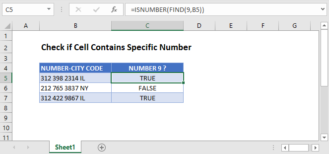
Check if Cell Contains Specific Number Using ISNUMBER and FIND

A cell that contains a mix of letters, numbers, spaces, and/or symbols is stored as a text cell in Excel. We can check if one of those cells contains a specific number with the ISNUMBER and FIND Functions.

=ISNUMBER(FIND(9,B3))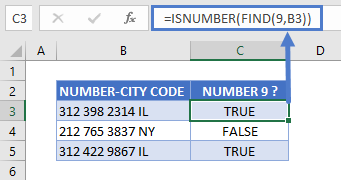

Let’s step through this two-part formula.

The FIND Function

First, the FIND Function checks for a specified character within a text string. It then returns the position of that character in the string, or a #VALUE! error if it is not found.

=FIND(9,B3)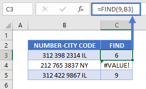

FIND

In this example, the FIND Function returns the position of “9” in each cell. As shown above, for cells without the number 9, it returns a VALUE error.

Note: You can use either the FIND or SEARCH Function to check if a cell contains a specific number. Both functions have the same syntax and, with numeric find texts, produce the same result.

The ISNUMBER Function

Next, the ISNUMBER Function does what its name implies: it checks if a cell is a number and returns TRUE or FALSE.

=ISNUMBER(C3)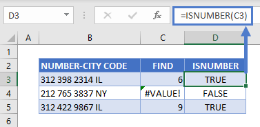

The ISNUMBER Function checks the result of the FIND Function and returns TRUE for cells with position numbers and FALSE for the cell with a VALUE error.

Combining these functions together gives us our original formula:

=ISNUMBER(FIND(9,B3))

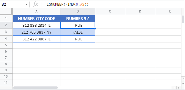
Check if Cell Contains Specific Number in Google Sheets

These functions work the same in Google Sheets as in Excel.

Источник

When working with Excel, we see so many peculiar situations. One of those situations is searching for the particular text in the cell. The first thing that comes to mind when we say we want to search for a specific text in the worksheet is the “Find and Replace” method in Excel, which is the most popular one. But Ctrl + F can find the text you are looking for but cannot go beyond that. So, for example, if the cell contains certain words, you may want the result in the next cell as “TRUE” or “FALSE.” So, Ctrl + F stops there.

How to Search For Text in Excel?
- Which Formula Can Tell Us A Cell Contains Specific Text?
- Alternatives to FIND Function
  - Alternative #1 – Excel Search Function
  - Alternative #2 – Excel Countif Function
- Highlight the Cell which has Particular Text Value
- Recommended Articles

You are free to use this image on your website, templates, etc, Please provide us with an attribution linkArticle Link to be Hyperlinked
For eg:
Source: Search For Text in Excel (wallstreetmojo.com)

Here, we will take you through the formulas to search for the particular text in the cell value and arrive at the result.

You can download this Search For Text Excel Template here – Search For Text Excel Template

Which Formula Can Tell Us A Cell Contains Specific Text?

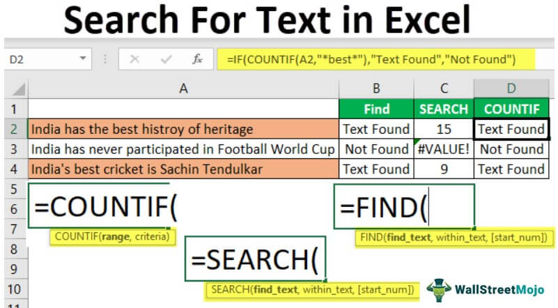
It is a question we have seen many times in Excel forums. The first formula that came to mind was the “FIND” function.

The FIND function can return the position of the supplied text values in the string. So, if the FIND method returns any number, then we can consider the cell as it has the text or else not.

For example, look at the below data.
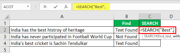
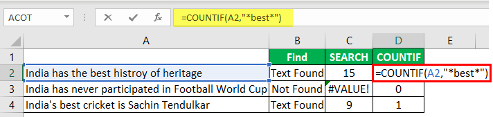
In the above data, we have three sentences in three different rows. Now in each cell, we need to search for the text “Best.” So, apply the FIND function.
The “find_text” argument mentions the text we need to find.
For the “within_text,” select the full sentence, i.e., cell reference.
The last parameter is not required to close the bracket and press the “Enter” key.

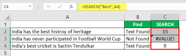
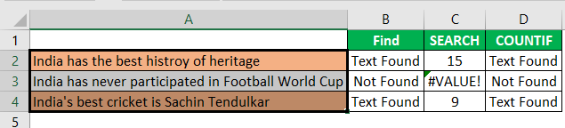
So, in two sentences, we have the word “best.” We can see the error value of #VALUE! in cell B2, which shows that cell A2 does not have the text value “best.”
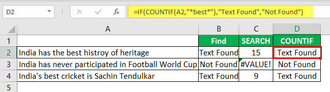
Instead of numbers, we can also enter the result in our own words. For this, we need to use the IF condition.

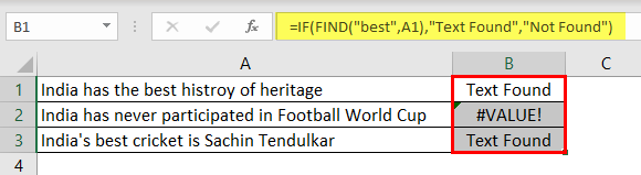
So, in the IF condition, we have supplied the result as “Text Found” if the value “best” is found. Otherwise, we have provided the result as “Not Found.”

But, here we have a problem, even though we have supplied the result as “Not Found,” if the text is still not found, we are getting the error value as #VALUE!.

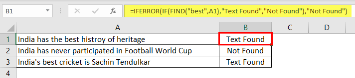
So, nobody wants to have an error value in their Excel sheet. Therefore, we must enclose the formula with the ISNUMERIC function to overcome this error value.

The ISNUMERIC function evaluates whether the FIND function returns the number or not. If the FIND function returns the number, it will supply TRUE to the IF condition or else FALSE condition. Based on the result provided by the ISNUMERIC function, the IF condition will return the result accordingly.

We can also use the IFERROR function in excelThe IFERROR function in Excel checks a formula (or a cell) for errors and returns a specified value in place of the error.read more to deal with error values instead of ISNUMERIC. For example, the below formula will also return “Not Found” if the FIND function returns the error value.

Alternatives to FIND Function

Alternative #1 – Excel Search Function

Instead of the FIND function, we can also use the SEARCH function in excelSearch function gives the position of a substring in a given string when we give a parameter of the position to search from. As a result, this formula requires three arguments. The first is the substring, the second is the string itself, and the last is the position to start the search.read more to search the particular text in the string. The syntax of the SEARCH function is the same as the FIND function.

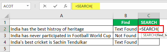
Supply the “find_text” as “Best.”

The “within_text” is our cell reference.

Even the SEARCH function returns an error value as #VALUE! If the finding text “best” is not found. As we have seen above, we need to enclose the formula with ISNUMERIC or IFERROR functions.

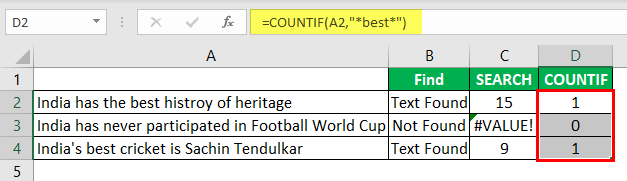
Alternative #2 – Excel Countif Function

Another way to search for a particular text is using the COUNTIF functionThe COUNTIF function in Excel counts the number of cells within a range based on pre-defined criteria. It is used to count cells that include dates, numbers, or text. For example, COUNTIF(A1:A10,”Trump”) will count the number of cells within the range A1:A10 that contain the text “Trump”
read more. This function works without any error.

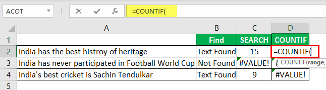
In the range, the argument selects the cell reference.

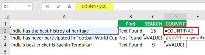
In the criteria column, we need to use a wildcard in excelIn Excel, wildcards are the three special characters asterisk, question mark, and tilde. Asterisk denotes multiple characters, a question mark denotes a single character, and a tilde denotes the identification of a wild card character.read more because we are just finding the part of the string value, so enclose the word “best” with an asterisk (*) wildcard.

This formula will return the word “best” count in the selected cell value. Since we have only one “best” value, we will get only 1 as the count.

We can apply only the IF condition to get the result without error.

Highlight the Cell which has a Particular Text Value

If you are not a fan of formulas, you can highlight the cell with a particular word. For example, to highlight the cell with the word “best,” we need to use conditional formatting in excelConditional formatting is a technique in Excel that allows us to format cells in a worksheet based on certain conditions. It can be found in the styles section of the Home tab.read more.

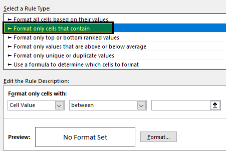
First, select the data cells and click “Conditional Formatting” > “New Rule.”

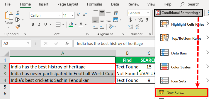
Under “New Rule,” select the “Format only cells that contain” option.

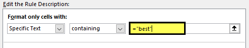
From the first dropdown, select “Specific Text.”

The formula section enters the text we search for in double quotes with the equal sign. =’best.’

Then, click on “FORMAT” and choose the formatting style.

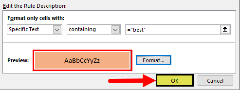
Click on “OK.” It will highlight all the cells which have the word “best.”

Using various techniques, we can search the particular text in Excel.