
Excel provides a variety of statistical functions, which we list below. Since these have been covered in the rest of the website, we won’t go into any detail here.
 Figure 1 – Basic Excel statistics functions
Click below for more information about each of these functions:
AVERAGE, MEDIAN, MODE, GEOMEAN, HARMEAN, AVEDEV, DEVSQ, STDEV, STDEVP, VAR, VARP, KURT, SKEW, LARGE, MAX, MIN, PERCENTRANK, PERCENTILE, QUARTILE, RANK, SMALL, AVERAGEIF, AVERAGEIFS, COUNT, STANDARDIZE, TRIMMEAN
Correlation and covariance functions
 Figure 2 – Excel correlation and covariance functions
Click below for more information about each of these functions:
CORREL, COVAR, PEARSON, RSQ, FISHER, FISHERINV
Regression function
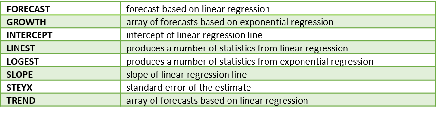 Figure 3 – Excel regression functions
Click below for more information about each of these functions:
FORECAST, INTERCEPT, SLOPE, TREND, LINEST, STEYX, GROWTH, LOGEST
Other statistical functions
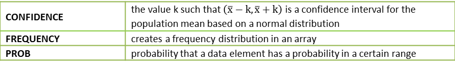 Figure 4 – Other Excel statistical functions
Click below for more information about each of these functions:
CONFIDENCE, FREQUENCY, PROB
Statistical distribution functions
The following table provides a list of the distributions supported by Excel. For each, the name of cumulative distribution functions (CDF) is given, and where available the name of the inverse function is also provided. For a few of the distributions, the CDF function also has an option to provide the probability density function (PDF). Finally, additional test functions are listed where available.
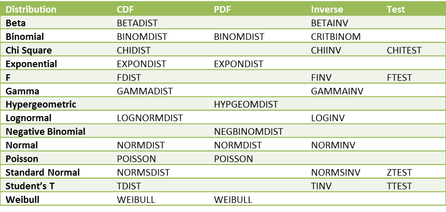
Figure 5 – Excel 2007 distribution functions
Excel 2010 functions
All the functions defined in previous versions of Excel are available in Excel 2010 and later versions of Excel, but the mathematical accuracy of many of these functions has been improved in Excel 2010 and later versions. In addition, a few new functions have been added and more consistent naming conventions have been introduced, including the following:
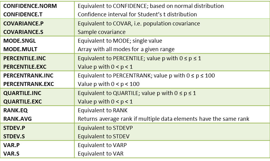 Figure 6 – New Excel 2010 statistical functions
For example, if R = {4,6,4,7,6,6}, then RANK(4,R) = 5, RANK(6,R) = 2 and RANK(7,R) = 1, while RANK.AVG(4,R) = 5.5, RANK.AVG(6,R) = 3 and RANK.AVG(7,R) = 1. Also RANK.EQ is the same as RANK. Similarly, RANK(4,R,1) = 1, RANK(6,R,1) = 3 and RANK(7,R,1) = 6, while RANK.AVG(4,R,1) = 1.5, RANK.AVG(6,R,1) = 4 and RANK.AVG(7,R,1) = 6.
MODE.MULT is an array function that is useful with multimodal data. Before using the function you need to highlight a vertical range (i.e. column vector) with at least as many cells as modes and then enter =MODE.MULT(R) and Ctrl-Shft-Enter (or simply Enter if using Excel 365). If you highlight more cells than modes the extra cells will contain the error values #N/A.
The function GAMMALN.PRECISE, which is equivalent to GAMMALN, has also been added in Excel 2010.
Starting with Excel 2010 there are the following alternative names for the distribution functions:
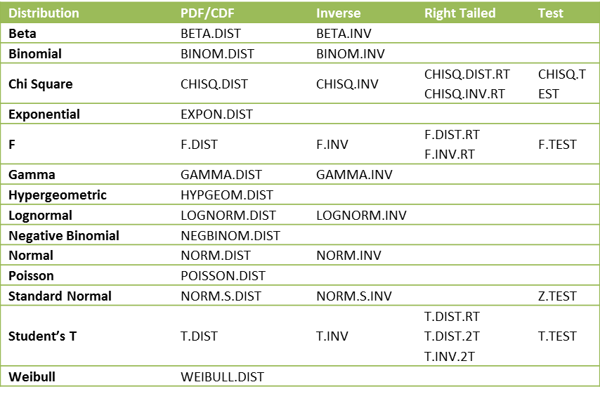 Figure 7 – Excel 2010 distribution functions
The functions that end in .DIST all provide both the probability distribution function (when the cum parameter is FALSE) as well as the left-tailed cumulative distribution function (when the cum parameter is TRUE). These are all left-tailed functions. For the chi-square and F distributions, there is also a right-tailed version (indicated by .RT in the above table) of the distribution and inverse cumulative functions. There is also a right-tailed version of the distribution function and a two-tailed version of the t distribution and its inverse.
The syntax for the various new t distribution functions is T.DIST(x,df,cum), T.DIST.RT(x,df) and T.DIST.2T(x,df). The syntax for the new inverse function is T.INV(p,df) and T.INV.2T(p,df). We have the following equivalences between the Excel 2007 and later versions of the t distribution functions:
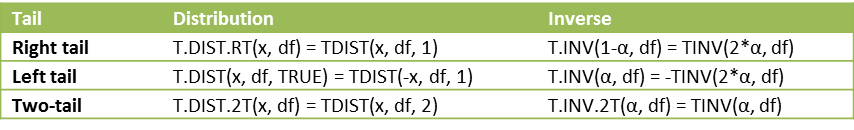 Figure 8 – Equivalences for the t distribution
Note that while the old t distribution functions worked differently from the normal and binomial distribution functions, the new functions are all consistent. Also, we can now explicitly calculate the pdf of the t distribution as T.DIST(x, df, FALSE) instead of having to use a complicated formula based on Definition 1 of t Distribution.
We also have the following equivalences between the Excel 2007 and later versions of the chi-square distribution functions:
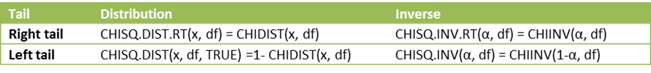 Figure 9 – Equivalences for the chi-square distribution
Finally, we can now explicitly calculate the pdf of the chi-square distribution as CHISQ.DIST(x, df, FALSE). The equivalences for the F distribution between Excel 2007 and later versions are similar.

Figure 10 – Equivalences for the F distribution
Excel 2013 functions
All the functions defined in previous versions of Excel are available in Excel 2013, but the following additional functions are available in versions of Excel starting with Excel 2013:
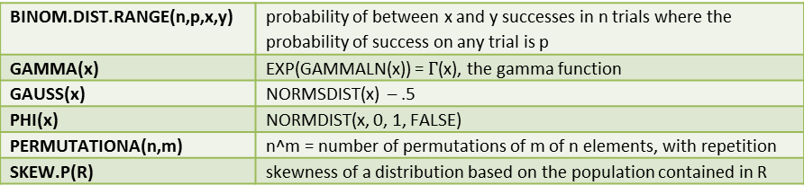 Figure 11 – New Excel 2013 statistical functions
Excel 2016 forecast functions
The following forecast functions were introduced with Excel 2016. More details about these functions can be found at Excel 2016 Forecasting Functions.
FORECAST.ETS(x, R1, R2, seasonality, missing, aggregation) = the forecasted value at the time value x
FORECAST.ETS.SEASONALITY(R1, R2, missing, aggregation) = the seasonality value (1 for no seasonality, 4 for quarterly, 12 for monthly, etc.) based on the data in R1 and R2
FORECAST.CONFINT(x, R1, R2, 1 – α, seasonality, missing, aggregation) = k such that (x-pred – k, x-pred + k) is the 1 – α confidence interval for the forecasted value x–pred at the time value x; the default value for 1 – α is .95.
FORECAST.ETS.STAT(R1, R2, stat-type, seasonality, missing, aggregation) = a forecasted statistic based on the value of stat-type.
In addition, the FORECAST.LINEAR function has been added that is equivalent to the FORECAST function described in Figure 3 above.
Reference
Microsoft (2021) Excel functions
https://support.microsoft.com/en-us/office/excel-functions-alphabetical-b3944572-255d-4efb-bb96-c6d90033e188#bm6
In the modern data-driven business world, we have sophisticated software dedicatedly to working towards “Statistical Analysis.” Amidst all these modern, technologically advanced excel software is not a bad tool to do your statistical analysis of the data. Of course, we can do all statistical analysis using Excel, but you should be an advanced Excel user. This article will show you some basic to intermediate-level statistics calculations using Excel.
Table of contents
- Excel Statistics
- How to use Excel Statistical Functions?
- #1: Find Average Sale per Month
- #2: Find Cumulative Total
- #3: Find Percentage Share
- #4: ANOVA Test
- Things to Remember
- Recommended Articles
- How to use Excel Statistical Functions?
How to use Excel Statistical Functions?
You can download this Statistics Excel Template here – Statistics Excel Template
#1: Find Average Sale per Month
The average rate or trend is what the decision-makers look at when they want to make crucial and quick decisions. So finding the average sales, cost, and profit per month is a common task everybody does.
For example, look at the below data of monthly sales value, cost value, and profit value columns in Excel.

So, by finding the average per month from the whole year, we can see what per month numbers are.
Using the AVERAGE functionThe AVERAGE function in Excel gives the arithmetic mean of the supplied set of numeric values. This formula is categorized as a Statistical Function. The average formula is =AVERAGE(read more, we can find the average values from 12 months, which boils down to per month on an average.
- Open the AVERAGE function in the B14 cell.

- Select the values from B2 to B13.

- The average value for sales is:

- Copy and paste cell B14 to the other two cells to get the average cost and profit. The average value for the cost is:

- The average value for the profit is:

So, on average, per month, the sale value is $25,563, the cost value is $24,550, and the profit value is $1,013.
#2: Find Cumulative Total
Finding the cumulative total is another set of calculations in excel statistics. Cumulative is nothing but adding all the previous month’s numbers together to find the current total for the period.
The steps to find the cumulative total are as follows:
- First, look at the below 6 months sales numbers.

- Open the SUM function in the C2 cell.

- Select the cell B2 cell and make the range reference.

From the range of cells, make the first part of the cell reference B2 an absolute reference by pressing the F4 key. - Close the bracket and press the “Enter” key.

- Drag and drop the formula below one cell.

- Now, we have the first two months’ cumulative total. At the end of the first two months, revenue was $53,835. Drag and drop the formula to other remaining cells.

From this cumulative, we can find in which month there was a less revenue increase.


Out of twelve months, you may have got $1,000,000 in revenue. But, still, maybe in one month, you must have achieved the majority of the revenue, and finding the month’s percentage share helps us find the particular month’s percentage share.
For example, look at the below data of the monthly revenue.

To find the percentage share first, we need to see what the overall 12 months total is, so by applying the SUM function in excelThe SUM function in excel adds the numerical values in a range of cells. Being categorized under the Math and Trigonometry function, it is entered by typing “=SUM” followed by the values to be summed. The values supplied to the function can be numbers, cell references or ranges.read more, find the overall sales value.

We can use the formula to find the percentage share of each month.
% Share = Current Month Revenue / Overall Revenue
To apply the formula as B2 / B14.

The percentage share for Jan month is:

Note: Make the overall sales total cell (B14 cell) an absolute referenceAbsolute reference in excel is a type of cell reference in which the cells being referred to do not change, as they did in relative reference. By pressing f4, we can create a formula for absolute referencing.read more because this cell will be a common divisor value across 12 months.
Copy and paste the C2 cell to the below cells as well.

Apply the “Percentage” format to convert the value to percentage values.

So, from the above percentage share, we can identify that the “Jun” month has the highest contribution to overall sales value, i.e., 11.33%, and the “May” month has the lowest contribution to overall sales value, i.e., 5.35%.

#4: ANOVA Test
Analysis of Variance (ANOVA) is the statistical tool in excel used to find the best available alternative from the lot. For example, if you are introducing four new kinds of food to the market. You gave a sample of each food to get the public’s opinion and from the opinion score given by the public by running the ANOVA test. We can choose the best from the lot.
ANOVA is a data analysis tool available in Excel under the “DATA” tab. By default, it is not available. You need to enable it.

Below are the scores of three students from 6 different subjects.

Click on the “Data Analysis” option under the “Data” tab. It will open up below the “Data Analysis” tab.

Scroll up and choose “Anova: Single Factor.”

Choose “Input Range” as B1 to D7 and tick “Labels in first row.”

Select the “Output Range” as any of the cells in the same worksheet.

We will have an “ANOVA” analysis ready.

Things to Remember
- All the basic and intermediate statistical analyses are possible in Excel.
- We have formulas under the category of “Statistical” formulas.
- If you are from a statistics background, it is easy to do fancy and important statistical analyses in Excel like T-TEST, Z-TEST, Descriptive StatisticsDescriptive statistics is used to summarize information available in statistics, and there is a descriptive statistics function in Excel as well. This built-in tool is found in the data tab, in the data analysis section.read more,” etc.
Recommended Articles
This article is a guide to statistics in excel. Here, we discuss using Excel statistical functions, practical examples, and a downloadable Excel template. You may learn more about Excel from the following articles: –
- Group Data in Excel
- Excel Convert Function
- Median FormulaThe median formula in statistics is used to determine the middle number in a data set that is arranged in ascending order. Median ={(n+1)/2}thread more
- Formula of Arithmetic Mean
To begin with, statistical function in Excel let’s first understand what is statistics and why we need it? So, statistics is a branch of sciences that can give a property to a sample. It deals with collecting, organizing, analyzing, and presenting the data. One of the great mathematicians Karl Pearson, also the father of modern statistics quoted that, “statistics is the grammar of science”.
We used statistics in every industry, including business, marketing, governance, engineering, health, etc. So in short statistics a quantitative tool to understand the world in a better way. For example, the government studies the demography of his/her country before making any policy and the demography can only study with the help of statistics. We can take another example for making a movie or any campaign it is very important to understand your audience and there too we used statistics as our tool.
Ways to approach statistical function in Excel:
In Excel, we have a range of statical functions, we can perform basic mead, median mode to more complex statistical distribution, and probability test. In order to understand statistical Functions we will divide them into two sets:
- Basic statistical Function
- Intermediate Statistical Function.
Statistical Function in Excel
Excel is the best tool to apply statistical functions. As discussed above we first discuss the basic statistical function, and then we will study intermediate statistical function. Throughout the article, we will take data and by using it we will understand the statistical function.
So, let’s take random data of a book store that sells textbooks for classes 11th and 12th.
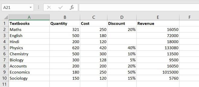
Example of statistical function.
Basic statistical Function
These are some most common and useful functions. These include the COUNT function, COUNTA function, COUNTBLANK function, COUNTIFS function. Let’s discuss one by one:
1. COUNT function
The COUNT function is used to count the number of cells containing a number. Always remember one thing that it will only count the number.
Formula for COUNT function = COUNT(value1, [value2], …)
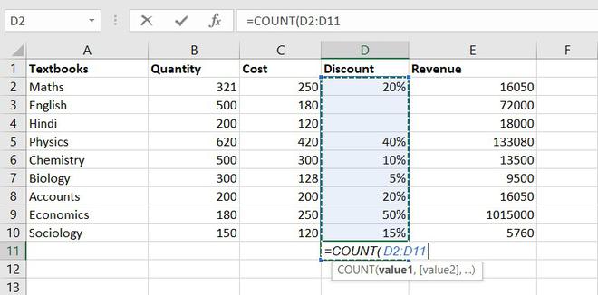
Example of statistical function.
Thus, there are 7 textbooks that have a discount out of 9 books.
2. COUNTA function
This function will count everything, it will count the number of the cell containing any kind of information, including numbers, error values, empty text.
Formula for COUNTA function = COUNTA(value1, [value2], …)
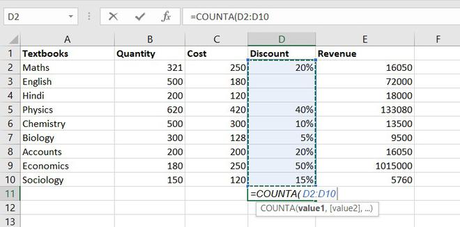
Example of statistical function.
So, there are a total of 9 subjects that being sold in the store
3. COUNTBLANK function
COUNTBLANK function, as the term, suggest it will only count blank or empty cells.
Formula for COUNTBlANK function = COUNTBLANK(range)
![]()
Example of statistical function.
There are 2 subjects that don’t have any discount.
4. COUNTIFS function
COUNTIFS function is the most used function in Excel. The function will work on one or more than one condition in a given range and counts the cell that meets the condition.
Formula for COUNTIFS function = COUNTIFS (range1, criteria1, [range2], [criteria2], ...)
Intermediate Statistical Function
Let’s discuss some intermediate statistical functions in Excel. These functions used more often by the analyst. It includes functions like AVERAGE function, MEDIAN function, MODE function, STANDARD DEVIATION function, VARIANCE function, QUARTILES function, CORRELATION function.
1. AVERAGE value1, [value2], …)
The AVERAGE function is one of the most used intermediate functions. The function will return the arithmetic mean or an average of the cell in a given range.
Formula for AVERAGE function = AVERAGE(number1, [number2], …)
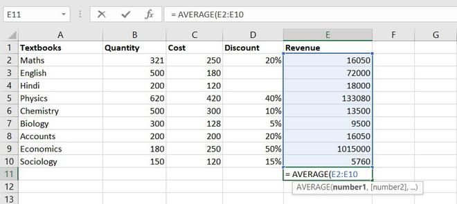
Example of statistical function.
So the average total revenue is Rs.144326.6667
2. AVERAGEIF function
The function will return the arithmetic mean or an average of the cell in a given range that meets the given criteria.
Formula for AVERAGEIF function = AVERAGEIF(range, criteria, [average_range])
3. MEDIAN function
The MEDIAN function will return the central value of the data. Its syntax is similar to the AVERAGE function.
Formula for MEDIAN function = MEDIAN(number1, [number2], …)
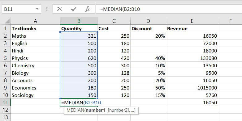
Example of statistical function.
Thus, the median quantity sold is 300.
4. MODE function
The MODE function will return the most frequent value of the cell in a given range.
Formula for MODE function = MODE.SNGL(number1,[number2],…)
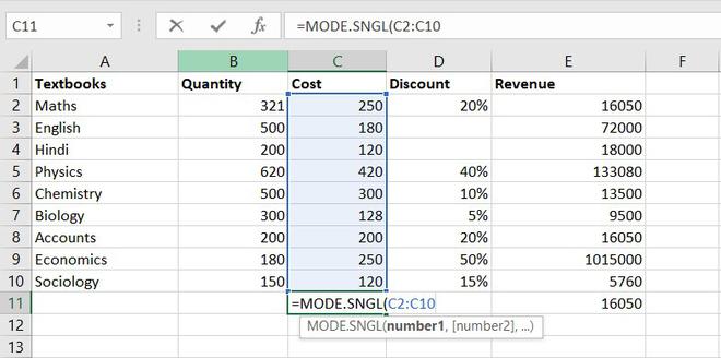
Example of statistical function.
Thus, the most frequent or repetitive cost is Rs. 250.
5. STANDARD DEVIATION
This function helps us to determine how much observed value deviated or varied from the average. This function is one of the useful functions in Excel.
Formula for STANDARD DEVIATION function = STDEV.P(number1,[number2],…)
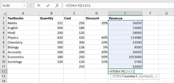
Example of statistical function.
Thus, Standard Deviation of total revenue =296917.8172
6. VARIANCE function
To understand the VARIANCE function, we first need to know what is variance? Basically, Variance will determine the degree of variation in your data set. The more data is spread it means the more is variance.
Formula for VARIANCE function = VAR(number1, [number2], …)
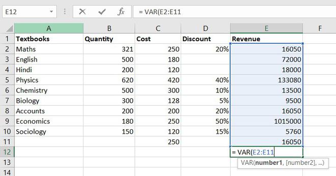
Example of statistical function.
So, the variance of Revenue= 97955766832
7. QUARTILES function
Quartile divides the data into 4 parts just like the median which divides the data into two equal parts. So, the Excel QUARTILES function returns the quartiles of the dataset. It can return the minimum value, first quartile, second quartile, third quartile, and max value. Let’s see the syntax :
Formula for QUARTILES function = QUARTILE (array, quart)
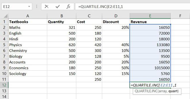
Example of statistical function.
So, the first quartile = 14137.5
8. CORRELATION function
CORRELATION function, help to find the relationship between the two variables, this function mostly used by the analyst to study the data. The range of the CORRELATION coefficient lies between -1 to +1.
Formula for CORRELATION function = CORREL(array1, array2)
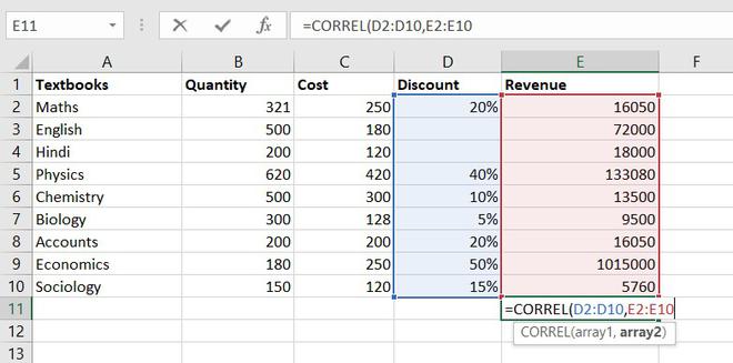
Example of statistical function.
So, the correlation coefficient between discount and revenue of store = 0.802428894. Since it is a positive number, thus we can conclude discount is positively related to revenue.
9. MAX function
The MAX function will return the largest numeric value within a given set of data or an array.
Formula for MAX function = MAX (number1, [number2], ...)
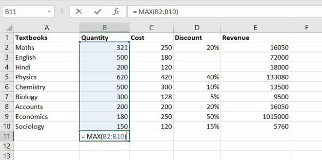
The maximum quantity of textbooks is Physics,620 in numbers.
10. MIN function
The MIN function will return the smallest numeric value within a given set of data or an array.
Formula for MIN function = MIN (number1, [number2], ...)
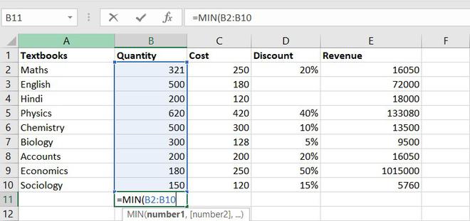
The minimum number of the book available in the store =150(Sociology)
11. LARGE function
The LARGE function is similar to the MAX function but the only difference is it returns the nth largest value within a given set of data or an array.
Formula for LARGE function = LARGE (array, k)
Let’s find the most expensive textbook using a large function, where k = 1
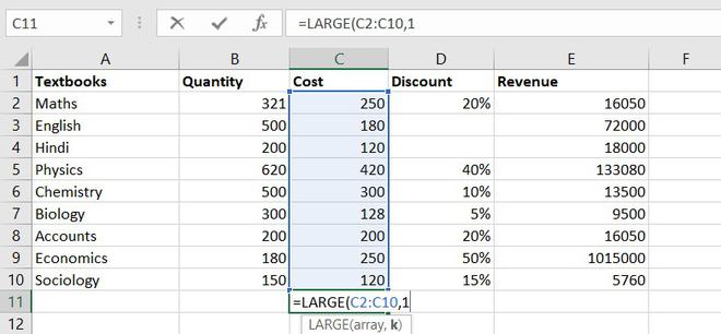
Example of statistical function.
The most expensive textbook is Rs. 420.
12. SMALL function
The SMALL function is similar to the MIN function, but the only difference is it return nth smallest value within a given set of data or an array.
Formula for SMALL function = SMALL (array, k)
Similarly, using the SMALL function we can find the second least expensive book.
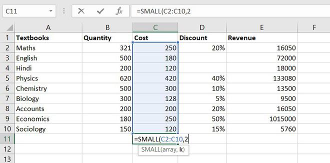
Example of statistical function.
Thus, Rs. 120 is the least cost price.
Conclusion
So these are some statistical functions of Excel. We have learned some of the most simple functions like COUNT functions to complex ones like the CORRELATION function. So far we learn, we understand how much these functions are useful for analyzing any data. You can explore more functions and learn more things of your own.
If you’re working with large datasets in excel, getting Descriptive Statistics for this data set could be useful.
Descriptive Statistic quickly summarizes your data and gives you a few data points that you can use to quickly understand the entire data set.
While you can also calculate each of these statistical values individually, using the descriptive statistics option in Excel quickly gives you all this data in one single place (and it’s a lot faster than using different formulas to calculate different values).
In this short tutorial, I will show you how to get Descriptive Statistics in Excel.
Descriptive Statistics in Excel
To get the Descriptive Statistics in Excel, you need to have the Data Analysis Toolpak enabled.
You can check whether you already have it enabled by going to the Data tab.
If you see the Data Analysis option in the Analysis group, you already have it enabled (and you can skip the next section and go directly to the ‘Getting Descriptive Analysis’ section).
In case you do not see the data analysis option in the data tab, follow the steps in the next section to enable it.
Enabling Data Analysis Toolpak
Below are the steps to enable the Data Analysis Toolpak in Excel:
- Open any Excel document
- Click the File tab

- Click on Options. This will open the Excel Options dialog box

- In the Excel Options dialog box, click on Add-ins in the left pane
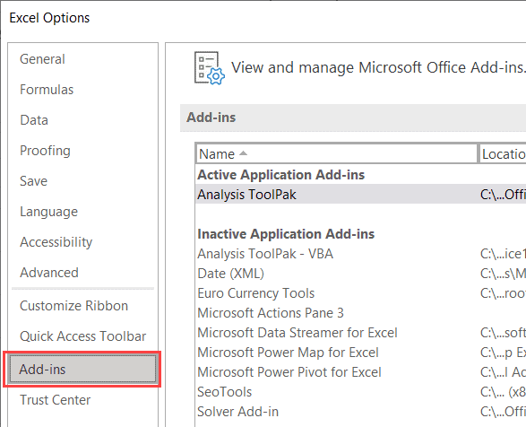
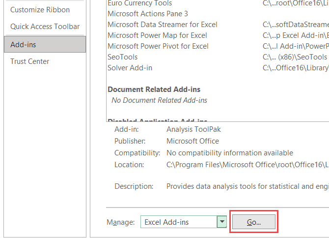
- From the Manage drop-down (which is at the bottom of the dialog box), select ‘Excel Add-ins’
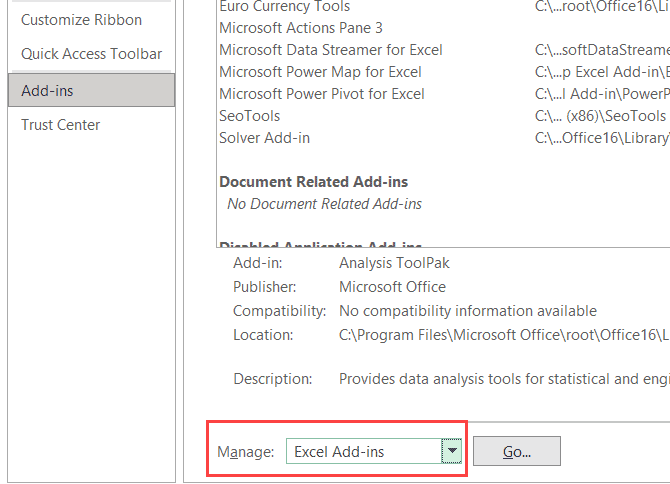
- Click on the Go button
- In the Add-ins dialog box that shows up, check the Analysis Toolpak option
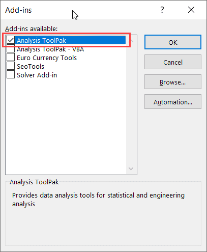
- Click OK
The other steps would enable the Data Analysis toolpak and you will be able to use it on all your Excel Workbooks.
Getting the Descriptive Analysis
Now that the Data Analysis Toolpak is enabled, let’s see how to get the descriptive statistics using it.
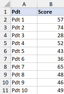
Suppose you have a data set as shown below where I have the sales data of different products of a company. For this data, I want to get descriptive statistics.
Below are the steps to do this:
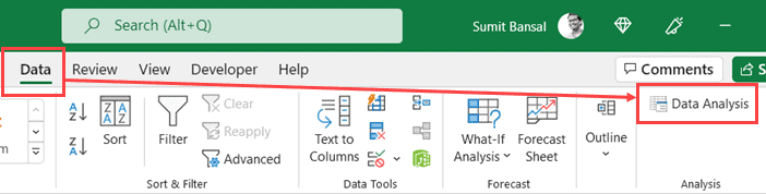
- Click the Data tab
- In the Analysis group, click on Data Analysis
- In the Data Analysis dialog box that opens, click on Descriptive Statistics
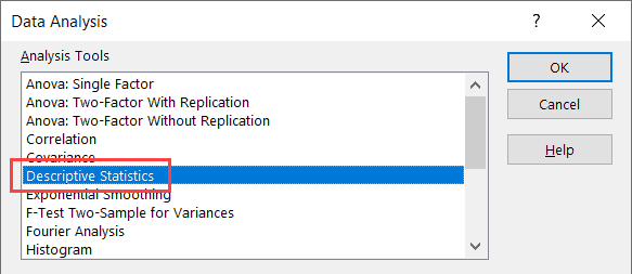
- Click OK
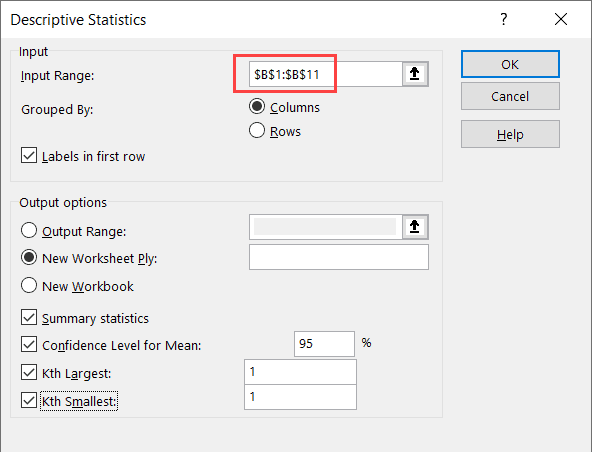
- In the Descriptive Statistics dialog box, specify the input range that has the data. Note that I have only used Column B as the data source (as you can only use numeric data as the input here)
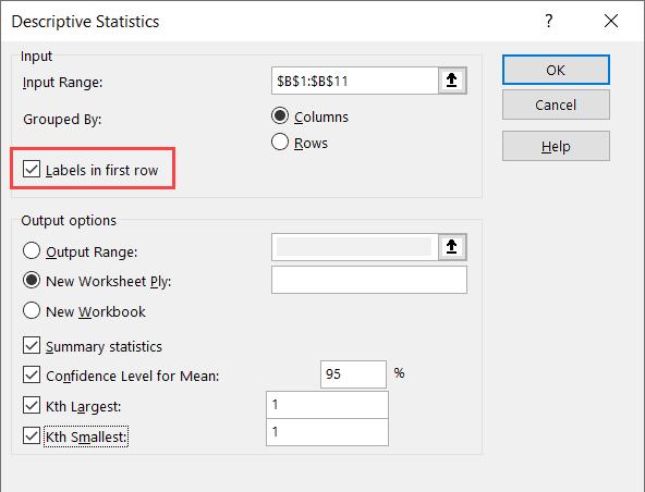
- If your data has headers, check the ‘Labels in first row’ option
- Select the New Worksheet Ply option (this will give the result in a new sheet)
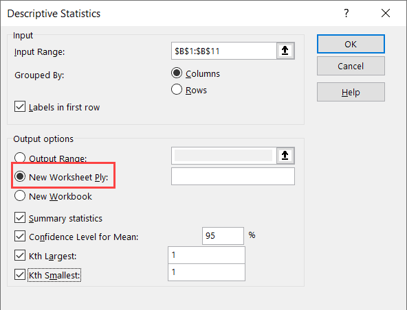
- Select the statistics options you want (you need to select atleast one, and can select all four)
- Click OK
The above steps would insert a new sheet and you will get the statistics as shown below:
Note that you can specify the following in step 8:
- Confidence Level for mean – the default is 95%, but you can change the value
- Kth Largest – the default is 1, but you can change it. If you enter 3 here, it will give you the third largest value from the dataset
- Kth Smallest – the default is 1, but you can change it. If you enter 3 here, it will give you the third smallest value from the dataset
Note that the resulting values you get are static values.
In case your original data changes and you again want to get the Descriptive Statistics, you will have to repeat the above steps again.
So this is how you can quickly get Descriptive Statistics in Microsoft Excel.
I hope you found this tutorial useful.
Other Excel Tutorials you may also like:
- How to Calculate Standard Deviation in Excel
- How to Calculate PERCENTILE in Excel
- Calculating Weighted Average in Excel.
- Calculating CAGR in Excel
- How to Calculate Correlation Coefficient in Excel
- Calculate the Coefficient of Variation (CV) in Excel
Using Excel for Statistical Analysis
MS Excel is one of the most commonly used tools for data analysis. The convenience of use and cost are two very important reasons why most data professionals prefer using Excel for statistical data analysis. However, using Excel for statistical analysis requires clarity of thought, data analysis knowledge, and strong decision-making skills.
Whether you are performing statistical analysis using Excel 2010 or Excel 2013, you need to have a clear understanding of charts and pivot tables. Most data analysts using Excel for statistical analysis depend largely on these two Excel features. Having knowledge of the essential statistics for data analysis using Excel answers is a plus.

Remember to install Data Analysis ToolPak if you are using Excel for statistical data analysis. In this discussion, we explain in detail the essential statistics for data analysis using Excel and how to perform descriptive analysis using Excel.
In this blog, I have tried to explore the functionalities of MS-Excel as a potential tool for statistical analysis and suggested some simple tricks and techniques that will save both time and energy.
Want to Know the Path to Become a
Data Science Expert?
Download Detailed Brochure and Get Complimentary access to Live Online Demo Class with Industry Expert
Date: 15th Apr, 2023 (Saturday) Time: 11:00 AM to 12:00 PM (IST/GMT +5:30)
Using Excel for Statistical Analysis: Pivot Tables
A PivotTable is an Excel tool for summarizing a list into a simple format. It helps you analyze all the data in your worksheet so as to make better business decisions. Excel can help you by recommending, and then, automatically creating PivotTables, which are a great way to summarize, analyze, explore, and present your data.

A pivot table may be used as an interactive data summarization tool to automatically condense large datasets into a separate, concise table. You can use it to create an informative summary of a large dataset or make regional comparisons between brand sales.

You can create PivotTables from lists, as you define which fields should be arranged in columns, which fields should become rows, and what data you wish to summarize.
Using Excel for Statistical Analysis: Descriptive Statistics
Descriptive Statistics tool in the Data Analysis add-in can be used on an existing data set to get up to 16 different descriptive statistics, without having to enter a single function on the worksheet. Descriptive Statistics gives you a general idea of trends in your data including:
- The mean, mode, median and range
- Variance and standard deviation
- Skewness
- Sample Variance
- Kurtosis and Skewness
- Count, maximum and minimum


Descriptive Statistics is useful because it allows you to take a large amount of data and summarize it. For example, you may want to represent the incomes of a community. Instead of showing it on an excel, you may summarize it, it becomes useful: an average wage, or a median income, is much easier to understand and then analyze the data.

You can find descriptive analysis by going to Excel→ Data→ Data Analysis → Descriptive statistics. It is the most basic set of analysis that can be performed on any data set.
Using Excel for Statistical Analysis: ANOVA (Analysis of Variance)
Analysis of variance (ANOVA) is a statistical technique that is used to check if the means of two or more groups are significantly different from each other. ANOVA checks the impact of one or more factors by comparing the means of different samples.

ANOVA method in Excel shows whether the mean of two or more data set is significantly different from each other or not. In other words, ANOVA analyses two or more groups simultaneously and finds out whether any relationship is there among the groups of data set or not.
For example, you may use ANOVA if you want to analyze the traffic of three different cities and find out which one is more efficient in handling the traffic (or if there are no significant differences among the traffic).

You will find three types of ANOVA in Excel:
- ANOVA single factor
- ANOVA two factor with replication
- ANOVA two factor without replication
If you have three groups of datasets and want to check whether there is any significant difference between these groups or not, you can use ANOVA single factor. If the P-value in the ANOVA summary table is greater than 0.05, you can say that there is a significant difference between the groups.
Using Excel for Statistical Analysis: Moving Average
Moving Average, another great tool for those using Excel for statistical analysis, is ideal for time series data such as stock price, weather report, attendance in class, etc. Moving Average is used extensively in stock price as a technical indicator. If you want to predict the stock price of today, the last ten days’ data would be more relevant than the last 1 year.
You may, simply plot the moving average of the stock having a 10-day period and then predict the estimated price. The same rule may be applied for predicting the temperature of a city. The recent temperature of a city can be calculated by taking the average of the last few weeks rather than the last few months.
Using Excel for Statistical Analysis: Rank and Percentile
The Rank and Percentile, another popular Excel features used for data analysis, is useful for finding the rank of all the values in a list. The best part of using the Rank and Percentile feature is that the percentile is also added to the output table.
The percentile is a percentage that indicates the proportion of the list which is below a given number. It calculates the ranking and percentile in the data set. For example, if you are managing a business of several products and want to find out which product is contributing to a higher revenue, you can use this rank method in Excel.
![]()
In the left table, we have our data on the revenues of different products. And we want to rank this data of products based on their revenue. With the help of rank and percentile, we can get the table shown on the right. You can observe that now the data is sorted and respective rank is also marked with each data.
Percentile shows the category in which the data belongs, such as the top 50%, top 30%, etc. In the summary table, the rank of product 7 is 4. As the total number of data is 7, we can easily say that it belongs to the top 50% of the data.
Using Excel for Statistical Analysis: Regression
Regression is one of the best features in Excel. It is widely used for using Excel for statistical data analysis. Regression is a process of establishing a relationship among many variables; to establish a relationship between dependent variables and independent variables.
Regression is great for use for using Excel for statistical data analysis. You, may, for example, want to see if there is an increase in the revenue of the product, which is not due to the increase in the advertisement.

If you performing statistical analysis using Excel 2010, Regression Analysis is the best way of mathematically sorting out which of those variables does indeed have an impact. It answers the questions: Which factors matter most? Which can we ignore? How do those factors interact with each other? And, perhaps most importantly, how certain are we about all of these factors?

These factors are more commonly known as variables. You may have your dependent or independent variables. In order to conduct a regression analysis, you gather the data on the variables in question.
You may take all of your monthly sales numbers, the past five years and any data on the independent variables you may find useful. You may, for example, find out the average monthly rainfall for the past five years as well.
Using Excel for Statistical Analysis: Random Number Generator
If you are using Excel for statistical data analysis, on a regular basis, Random Number Generator must be your top choice for generating a series of random numbers. This simple function in Excel gives you more flexibility in the random number generation process. It gives you more control over the generated data.


A random number is one that is drawn from a set of possible values, each of which is equally probable. In statistics, this is called a uniform distribution, because the distribution of probabilities for each number is uniform (i.e., the same) across the range of possible values.
For example, a good (unloaded) die has the probability 1/6 of rolling a one, 1/6 of rolling a two and so on. Hence, the probability of each of the six numbers coming up is exactly the same, so we say any roll of our die has a uniform distribution.
When discussing a sequence of random numbers, each number drawn must be statistically independent of the others. This means that drawing one value doesn’t make that value less likely to occur again. This is exactly the case with our unloaded die: If you roll a six, that doesn’t mean the chance of rolling another six changes.


Two very essential statistics for data analysis using Excel:
- The function RANDBETWEEN returns a random integer number
- The function RAND () returns a random real number of a uniform distribution. It will be less than 1 and greater than or equal to 0.
Using Excel for Statistical Analysis: Sampling
Sampling is one of the most readily preferred Excel tools if you are using Excel for statistical data analysis. This option is used for creating samples from a huge population. You can randomly select data from the dataset or select every nth item from the set.
For example, if you may want to measure the effectiveness of female call center employee in a call center, you can use this tool to randomly select few data every month and listen to their recorded calls and give a rating based on the selected call.

Sampling Methods:
If you are using statistical analysis using Excel 2010, you can make use of two sampling methods in Excel for retrieving or identifying items in your data set:
- Periodic: In this case, you specify the Period n at which you want sampling to take place. The nth value in the input range and every nth value thereafter is copied to the output column. Sampling stops when the end of the input range is reached.
- Random: In this case, you specify the Random Number of Samples. This number of values is drawn from random positions in the input range. A value can be selected more than once. (I.e. sampling is with replacement).
The data science field is booming to such an extent that our earlier analysis of employment reported that there are currently more than 97,000 job openings in India for analytics and information science. Thus, building a career in Data Science is quite in trend these days as the Data Science domain offers lucrative career options.
Excel is one of the most dynamic and intriguing tools for statistical analysis. We have discussed a few features. Play around with Excel to know more about other tools and techniques. You may also look for essential statistics for data analysis using Excel answers.
We offer one of the best-known courses in the Certified Data Analytics Course. The course enables you to learn tools such as Advanced Excel, PowerBI, and SQL. The live projects and intensive training program also empower you to come up with solutions for real-life problems.

Excel Statistics (Table of Contents)
- Introduction to Statistics in Excel
- Examples of Statistics in Excel
Introduction to Statistics in Excel
In this modern era where business solutions in a layman language are all people are thinking of, different dedicated software is developed and used for Statistical Analysis. It is a major part of the decision-making and finding out adequate solutions for your business problems. Despite the fact that it is not as powerful as the software designed dedicatedly for the Statistical Analysis, Excel still holds some of the power games to be able to do most of the Statistical Analytical tasks on its own and that too in a pretty simple manner. You need to be an advanced user of Excel, though, in order to be able to work on Statistical Analysis through Excel.
Examples of Statistics in Excel
We will see some examples using which we can calculate the statistics under Excel.
You can download this Statistics Excel Template here – Statistics Excel Template
Example #1 – Find Average
Suppose we have Country-wise Sales and Margin data as shown below:

We wanted to capture the average sales value for our company throughout these countries. The standard formula for Average is as below:
Average/Mean = Sum of All Values/ Number of Values
However, in Excel, you have a built-in AVERAGE function that does this task for you.
Step 1: In cell B9, start typing the formula =AVERAGE()

Step 2: Use B2:B7 (all sales values) as a reference under the AVERAGE function.

Step 3: Close the parentheses to complete the formula and press Enter key to see the output as shown below:

Step 4: Copy cell B9 and paste (Ctrl + V) it under cell C9 to get the average value for Margin. Well, this is one of the nicest Excel features of all time. You can copy the formulas and paste them to different cells so that you get the formulated results for the other column.

Example #2 – Margin Percentage for Each Country
Suppose we wanted to capture the Margin % we have acquired through business with each country. Does percentage show it all in a nice way, you know? Let’s see how this can be done.
The general formula for calculating Margin% is as follows:
Margin% = Margin/Sales
Step 1: In column D, under cell D2, use the formula as C2/B2 (Since C2 has Margin and B2 has Sales value for UAE).

Step 2: Press Enter key to see the Margin% value we have acquired for UAE through our trade.

Step 3: Now, Drag down this formula across the rows to see the Margin% we have acquired for different countries through trade. You can use the keyboard shortcut Ctrl + D to achieve the result. Select all the necessary sales, including D2 and press Ctrl + D.

We need to change the number formatting for column D to be seen in a percentage format. Follow the step below to achieve the result.
Step 4: Select entire column D. Go to Home tab, under which navigate towards Number group.

You can see the result as below:

Example #3 – Find Standard Deviation
We can also be very interested in knowing the degree to which the data points are deviating from our data. We can find out the Standard Deviation, which gives us a good idea about the spread of the data. It is very easy to calculate Standard Deviation under Excel. We have two functions to achieve the result.
STDEV.P and STDEV.S. STDEV.P works well when you have an entire population to cover, and STDEV.S is the one that can be used to figure out the Standard Deviation for a sample. Follow the steps below to be able to find the standard deviation.
Step 1: Start typing the formula under cell D10 as =STDEV.S( to initiate the formula for sample standard deviation.

Step 2: Now, use the range of cells you wanted to capture the standard deviation. I will use the sales values spread across B2:B7 as a reference to the STDEV.S function. It will give me a single value, which represents the standard deviation between the Sales Values.

Step 3: Use closing parentheses to complete the formula and press Enter key. You’ll get a Standard Deviation value as shown in the screenshot below:

Example #4 – Regression Analysis
Regression Analysis is a widely used statistical technique to determine a relationship between two or more variables and predict the future (forecasting) based on the model fitted. It assumes that there is some kind of relationship (termed as correlation) between two variables.
Suppose we have data of Height (in cm) and Weight (in kg) as shown below, and we are keen to know whether there is any relationship between both. If so, can we predict one based on the other?

This is a problem with Regression. Follow the steps below to run a regression analysis for the same.
Step 1: Navigate towards the Data tab and click on the Data Analysis button under the Analyze section.

Step 2: Once you click there, the Data Analysis toolbox will pop up. Scroll down to navigate towards and select Regression. Click OK.

Step 3: Use B2:B11 as Input Y Range and A2:A11 as Input X Range under the Regression window that pops up.

Step 4: Tick the Labels option, select Output Range as E2 of the current worksheet, and tick on Residuals to show the residuals for the data.

Step 5: Click the OK button once you are satisfied with the output options you chose. It is customizable; feel free to add some more residuals if you want.

You can see a regression output as shown in the image below under the same worksheet where data is present.

This is how we can use the statistical techniques in Excel to extract more analytical insights through our data. This article ends here.
Things to Remember
- There are more Statistical functions than the ones we have used in this article. Most of the formulae could be found under More Functions > Statistical functions encapsulated under Formulas sections.
- All basic Descriptive Statistics can also be calculated at once using Data Analysis Descriptive Statistics tool. This will capture Mean, Mode, Median, Range, Quartiles, Quartile Deviations, etc., for you at a single click.
- Working with advanced statistical techniques such as Regression, ANOVA, T-Test, F-Test, etc., is really very easy within Excel. I mean, come on! All you need to do is select an appropriate technique and do some clicking.’
Recommended Articles
This has been a guide to Statistics in Excel. Here we discuss How to use Statistics in Excel along with practical examples and a downloadable excel template. You can also go through our other suggested articles –
- Linear Interpolation in Excel
- Excel Regression Analysis
- Regression Line Formula
- Excel GROWTH Formula
Descriptive statistics with excel is a popular way to describe your data. It makes the tons of formula became easier just by simple click and drop.
Years ago, I do the formula one by one and find the statistic value that I need. It is really uncomfortable, is not it?
You have to remember the correct formula of your data and choose the right formula because perhaps there is more than one similar formula for one statistic value.
Look at he picture I present below. This is what you will using descriptive statistics with excel by typing the formula one by one

There are 7 formulas that excel provide to you to generate the variance of your data. My question is, which one will you use?
Still, writing one by one formula to summarize the statistic value that you need? Well, keep reading!
Microsoft Excel is a phenomenal software developed by Microsoft helping Billions of human to solve their problems. Excel helps us to makes almost our calculation problem easier included statistics.
Contents
- Why using descriptive statistics in excel?
- Steps of Descriptive Statistics With Excel
- Interpretation of Descriptive Statistics Output in Excel
- The Disadvantage of Using Excel For Descriptive Statistics
- You have to read this!
Why using descriptive statistics in excel?
If you are wondering why you should Microsoft Excel to process your statistical data, let me tell you these interesting facts!
1. The user interface is so friendly
Yes, Microsoft Excel interface is so friendly so almost every user could use it without any meaningful problem. You may use it through simple steps and clicks to produce the output that you want.
2. No coding needed
Usually, almost all statistical software needs to code the form. But, Excel does not require you to code anything. You just need to know the simple formula or use the toolbar that will help you to finish the job.
3. Easy to interpret
The output is served simply so we may see it and understand what the output is. If you did not strong statistical basics, do not worry. It’s just basic formula which you may learn in your study.
Before using Microsoft Excel to process your data, you must activate the data analysis toolpak to makes your job easier.
Follow these simple steps!
1. Activate the data analysis toolpak, go to file >> options

2. Choose add ins >> analysis toolpak
3. Ok
Now, you will have the tools that you need to make your works easier and faster. By using this toolpak, you do not have to input every single formula that you need. Now, let’s calculate the descriptive statistics in excel
Already have your data set? Let’s do the analysis. Here is the steps!
1. Go to Data >> data analysis

2. You’ll see many statistical options there, choose descriptive statistics >> ok

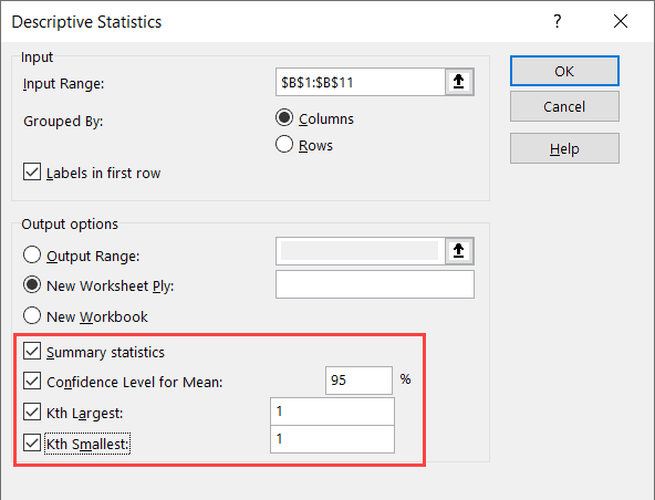
3. In the popup window, you have several fields that you have to fill

- Input range: block the data you want to analyze
- Grouped by: whether the data is grouped in columns or rows
- Labels in the first row: if the blocked data has labels in the first row, check this
- Output options: where the output will be displayed
- Summary statistics: if you want to do descriptive statistics analysis
- The confidence level for mean: if you want to show confidence level for mean
- Kth largest: if you want to show the data in “k”th largest
- Kth smallest: if you want to show the data in “k”th smallest
4. Click Ok
5. See the magic happens!

Interpretation of Descriptive Statistics Output in Excel
1. Mean = 7,434. In average, there are 7,434 poor people in these 12 areas
2. Standard error = 468.412. This value indicates that the sample we chose has a fairly high distribution of the population mean.
3. Median = 7,575. This value indicates that the middle numbers of poor people based on the sample we use are 7,575 people.
4. Mode = 8000. This value shows that the most number of poor people based on the sample we have is 8000 people.
5. Standard deviation = 1622. This value indicates that the sample values that we use are spread far enough from the mean value.
6. Kurtosis = -0.68485. Because the value of kurtosis is smaller than 3, we can conclude that the sample used is platicurtic distribution (tends to be flat).
7. Skewness = -0.12018. Because the skewness value is smaller than zero, we can conclude that the data tends to be left inclined or left skewed.
8. Range = 5100. This value indicates that the difference between the regions with the highest number of poor people and the lowest number of poor people is 5100 people.
9. Minimum = 4900. This value shows the lowest number of poor people is 4900 people in the L area.
10. Maximum = 10,000. This value shows that the highest number of poor people is 10,000 people in J area.
11. Sum = 89,210. This value indicates that the total number of poor people based on the data used was 89,210 people.
12. Count = 12. This value indicates the amount of data used is 12.
13. Confidence level = 1030,968. It’s quite difficult to understand, right? Okay, keep reading.
Confidence interval means we will predict a value in the form of a range. In this case, we need upper values and lower values.
In the descriptive statistics feature in Microsoft Excel, they only provide one value, and this figure is very far from the mean.
The confidence level value that appears is a value that can be used to get the upper and lower limits of the confidence interval you are using.
If you want to get the upper limit, you simply add an average to the value of the confidence level. The following calculations. Check the picture below!

If you want to get a lower bound value, you can simply reduce the average value with that confidence level. Consider the following picture.

Now, let’s make the interpretation of this value!
With a confidence level of 95 percent, the average number of poor people in the 12 regions is 6,403 to 8,465 people.
The Disadvantage of Using Excel For Descriptive Statistics
1. The formula is limited
Although the formula is super easy just by drag and click, the numbers of excel formula in the statistical process are limited.
Excel provided not much formula so the user can use to do data processing. But, Excel is the best tool to study statistical computing if you want to be advanced in the future.
2. It is only for numerical data
It’s sad but if you are using categorical or non-numeric data, probably excel is not for your research. Excel only read the data in numeric format. Even you transform it into numerical form, it’s quite difficult to read the output.
3. It is only for single variable analysis
Conclusion
Overall, the steps of using descriptive statistics in excel are:
1. Prepare the data set.
2. Activate analysis toolpak add-ins add options menu.
3. Choose the descriptive statistics at the data analysis menu.
4. Check the statistic value that you want to generate.
5. Click Ok.
6. Do not forget to make the output interpretation.
If you want to do more advanced analysis by software, I recommend you to check the descriptive statistics on spss article. You will find an easier way to produce the descriptive statistics even for the numerical or categorical data set.
You can use the Analysis Toolpak add-in to generate descriptive statistics. For example, you may have the scores of 14 participants for a test.

To generate descriptive statistics for these scores, execute the following steps.
1. On the Data tab, in the Analysis group, click Data Analysis.

Note: can’t find the Data Analysis button? Click here to load the Analysis ToolPak add-in.
2. Select Descriptive Statistics and click OK.

3. Select the range A2:A15 as the Input Range.
4. Select cell C1 as the Output Range.
5. Make sure Summary statistics is checked.

6. Click OK.
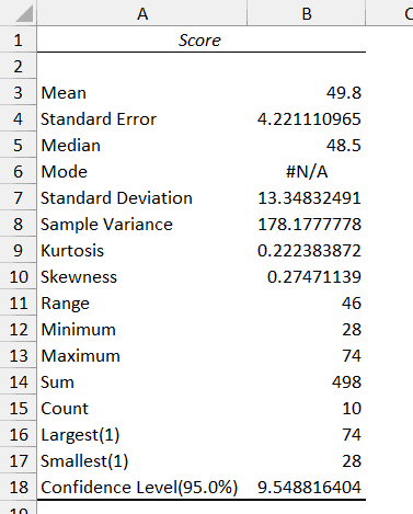
Result:

Tip: visit our page about statistical functions to learn more about this topic.