Using brackets in excel - Word и Excel - помощь в работе с программами

For certain purpose, may be sometimes, you need to insert brackets around the text within a cell to enclose the cell value. It is easy for you to insert brackets into a few cells, but, if there are lots of cells needed to be surrounded with brackets, how could you deal with the problem quickly and conveniently in Excel?

Insert brackets around text in a cell with formula

Insert brackets around text in a cell with VBA code

Insert brackets around text in a cell with Kutools for Excel

The following simple formula may help you to add the brackets around the text within a cell, please do as follows:

1. Please enter this formula =»(«&A2&»)» into a blank cell besides your data, C2, for instance, see screenshot:

2. Then press Enter key to get the result, and then select the cell C2, drag the fill handle down to the cells that you want to apply this formula, all the cell values have been inserted with the brackets around, see screenshot:

If you are familiar with the VBA code, I can create a VBA code for you to sole this task.

1. Hold down ALT + F11 keys in Excel, and it opens the Microsoft Visual Basic for Applications window.

2. Click Insert > Module, and paste the following code in the Module Window.

VBA code: Insert brackets around text in a cell

Sub addbrackets()
'Updateby20150706
Dim Rng As Range
Dim WorkRng As Range
On Error Resume Next
xTitleId = "KutoolsforExcel"
Set WorkRng = Application.Selection
Set WorkRng = Application.InputBox("Range", xTitleId, WorkRng.Address, Type:=8)
For Each Rng In WorkRng
Rng.Value = "(" & Rng.Value & ")"
Next
End Sub

3. Then press F5 key to execute this code, a prompt box is popped out to remind you selecting the data range that you want to add the brackets, see screenshot:

4. And then click OK, all the selected cells have been inserted brackets around at once.

If you are interested in other handy add-ins for Excel, Kutools for Excel may do you a favor, with its Add Text function, you can quickly add any characters into the cell contents at any position.

After installing Kutools for Excel, please do as follows:

1. Select the data range that you want to insert brackets.

2. Click Kutools > Text > Add Text, see screenshot:

3. In the Add Text dialog box, enter the half opening bracket “(” into the Text box, and then select Before first character under the Position, then click Apply button, see screenshot:

4. The half opening brackets have been inserted before each selected text value, and the dialog box is still opened, go on entering the half closing bracket “)” into the Text box, and select the After last character option, then click Ok button, see screenshot:

5. And the brackets have been inserted into the cell values.

Note:

With this Add Text feature, you can also insert the brackets into any position of the cell contents. For Example, I want to insert the brackets around the text after the fourth character of the cell, please do as follows:

1. In the Add Text dialog box, please type the half opening bracket “(” into the Text box, and choose Specify option, then enter the specific number of the position that you want to insert the bracket, and then click Apply button to finish this step, see screenshot:

2. Then insert the half closing bracket “)”into the Text box, and choose After last character option, and now, you can preview the results, in the right list box, see screenshot:

3. At last, click Ok button to close this dialog, and the brackets have been inserted around the text at specific position as you need.

Tips: If you check Skip non-text cells option in the dialog, the adding text won’t be inserted into the non-text cells.

Click to know more details about this Add Text feature.

Download and free trial Kutools for Excel Now !

Kutools for Excel: with more than 200 handy Excel add-ins, free to try with no limitation in 60 days. Download and free trial Now!

The Best Office Productivity Tools

Kutools for Excel Solves Most of Your Problems, and Increases Your Productivity by 80%

Reuse: Quickly insert complex formulas, charts and anything that you have used before; Encrypt Cells with password; Create Mailing List and send emails…
Super Formula Bar (easily edit multiple lines of text and formula); Reading Layout (easily read and edit large numbers of cells); Paste to Filtered Range…
Merge Cells/Rows/Columns without losing Data; Split Cells Content; Combine Duplicate Rows/Columns… Prevent Duplicate Cells; Compare Ranges…
Select Duplicate or Unique Rows; Select Blank Rows (all cells are empty); Super Find and Fuzzy Find in Many Workbooks; Random Select…
Exact Copy Multiple Cells without changing formula reference; Auto Create References to Multiple Sheets; Insert Bullets, Check Boxes and more…
Extract Text, Add Text, Remove by Position, Remove Space; Create and Print Paging Subtotals; Convert Between Cells Content and Comments…
Super Filter (save and apply filter schemes to other sheets); Advanced Sort by month/week/day, frequency and more; Special Filter by bold, italic…
Combine Workbooks and WorkSheets; Merge Tables based on key columns; Split Data into Multiple Sheets; Batch Convert xls, xlsx and PDF…
More than 300 powerful features. Supports Office / Excel 2007-2021 and 365. Supports all languages. Easy deploying in your enterprise or organization. Full features 30-day free trial. 60-day money back guarantee.

Office Tab Brings Tabbed interface to Office, and Make Your Work Much Easier

Enable tabbed editing and reading in Word, Excel, PowerPoint, Publisher, Access, Visio and Project.
Open and create multiple documents in new tabs of the same window, rather than in new windows.
Increases your productivity by 50%, and reduces hundreds of mouse clicks for you every day!

Источник

Sometimes we need to add brackets into cells to enclose texts for some reasons. If we only add brackets for one single cell, it is very easy, but if there are a column of cells need to add brackets, how can we do? This article will show you three simple ways to add brackets by Formula, Format Cells Function and VBA code.

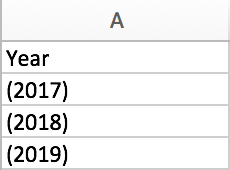
In condition, we prepare a table to save Year.

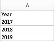
We use this sample to do demonstration.

Step 1: Select another column for example column B, in cell B2 enter =”(“&A2&”)”.

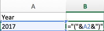
Step 2: Press Enter to get result.

Step 3: Select cell B2 which contains the formula, drag it and fill the cells B3 and B4. Then we can get a new column with brackets enclose the texts. You can copy the result to cover column A by paste with value.

Add Brackets for Cells by Format Cells Function in Excel

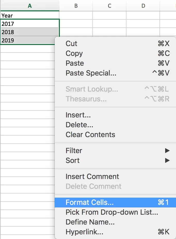
Step 1: Select all ranges you want to add brackets for them. In this case select A2, A3 and A4.

Step 2: Right click your mouse, select ‘Format Cells…’.

Step 3: On Format Cells window, select Custom under Category list.

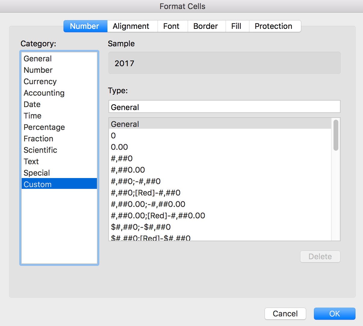
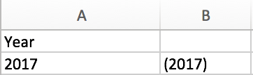
Step 4: In Type, enter “(“General”)”. Then you can find 2017 is changed to (2017) in Sample.

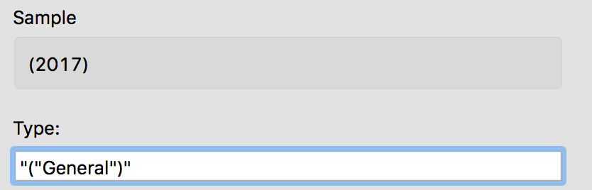
If the value in cell is Text, you can enter “(“@”)” in type instead.

Step 5: Click OK to get result. All cells are enclosed with brackets properly.

Add Brackets for Cells by VBA Code in Excel

Step1: open your excel workbook and then click on “Visual Basic” command under DEVELOPER Tab, or just press “ALT+F11” shortcut.

Step2: then the “Visual Basic Editor” window will appear.

Step3: click “Insert” ->”Module” to create a new module.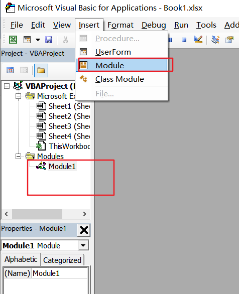

Step4: paste the below VBA code into the code window. Then clicking “Save” button.

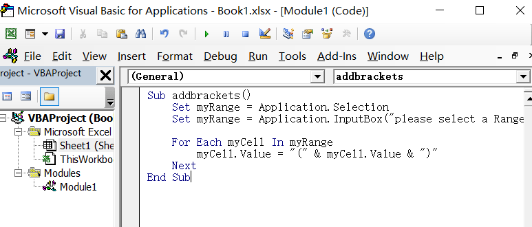
Sub addbrackets()
    Set myRange = Application.Selection
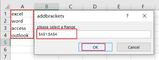
    Set myRange = Application.InputBox("please select a Range", "addbrackets", myRange.Address, Type:=8)

    For Each myCell In myRange
        myCell.Value = "(" & myCell.Value & ")"
    Next
End Sub

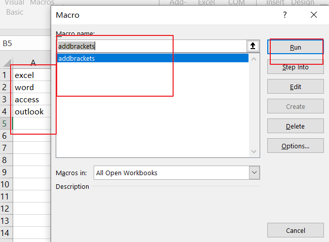
Step5: back to the current worksheet, click on Macros button under Code group. then click Run button.

Step6: you need to type one password to protect your current worksheet, click on Ok button.

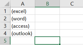
Step7: you would see that the selected cells have been inserted brackets around text.

Источник

To satisfy certain requirements, you may need to insert some curly braces into Word document or Excel spreadsheet. But in addition to regular curly braces, sometimes the curly braces with customized size that can contain several lines of text are also needed. In this post, I’ll introduce 4 commonly used methods to insert both regular and customized curly braces. The screeenshots are based on Word, but the steps are almost the same in Excel.

1. Keyboard Input

For regular curly braces, you can find the corresponding keys on the keyboard. Just hit the right key while pressing and holding [Shift], and the curly braces will be entered immediately.

2. Insert Equation

Go to Insert tab, click Equation in Symbols section.

You will be guided to Design (Equation Tools) tab then. Click Bracket to expand the drop-down menu. Here you can find all kinds of brackets, just select the curly braces (or single curly brace) to insert it.

3. Insert Shapes

Switch to Insert tab and choose Shapes. You can find the curly braces under Basic Shapes. It’s ok if you only want the left bracket or right bracket of it, just choose the corresponding bracket.

The brackets inserted in this way can be customized as you like. Drag the border to adjust its size, direction and location till you are happy with the result. Moreover, you can even change its color and effect.

4. Microsoft Equation 3.0

Go to Insert tab and choose Object > Object…

Select Microsoft Equation 3.0 in the list of Object type under the Create New tab. Click OK to implement it.

Then the Microsoft Equation tool will pop out. Click the bracket icon on the bottom-left corner to expand the menu, and select the curly braces in the list. It will be inserted to your document immediately.

Copyright Statement: Regarding all of the posts by this website, any copy or use shall get the written permission or authorization from Myofficetricks.

Источник

When you create an Excel table, Excel assigns a name to the table, and to each column header in the table. When you add formulas to an Excel table, those names can appear automatically as you enter the formula and select the cell references in the table instead of manually entering them. Here’s an example of what Excel does:

Instead of using explicit cell references	Excel uses table and column names
=Sum(C2:C7)	=SUM(DeptSales[Sales Amount])

That combination of table and column names is called a structured reference. The names in structured references adjust whenever you add or remove data from the table.

Structured references also appear when you create a formula outside of an Excel table that references table data. The references can make it easier to locate tables in a large workbook.

To include structured references in your formula, click the table cells you want to reference instead of typing their cell reference in the formula. Let’s use the following example data to enter a formula that automatically uses structured references to calculate the amount of a sales commission.

Sales Person	Region	Sales Amount	% Commission
Joe	North	260	10%
Robert	South	660	15%
Michelle	East	940	15%
Erich	West	410	12%
Dafna	North	800	15%
Rob	South	900	15%

Copy the sample data in the table above, including the column headings, and paste it into cell A1 of a new Excel worksheet.
To create the table, select any cell within the data range, and press Ctrl+T.
Make sure the My table has headers box is checked, and click OK.
In cell E2, type an equal sign (=), and click cell C2.

In the formula bar, the structured reference [@[Sales Amount]] appears after the equal sign.
Type an asterisk (*) directly after the closing bracket, and click cell D2.

In the formula bar, the structured reference [@[% Commission]] appears after the asterisk.
Press Enter.

Excel automatically creates a calculated column and copies the formula down the entire column for you, adjusting it for each row.

What happens when I use explicit cell references?

If you enter explicit cell references in a calculated column, it can be harder to see what the formula is calculating.

In your sample worksheet, click cell E2
In the formula bar, enter =C2*D2 and press Enter.

Notice that while Excel copies your formula down the column, it doesn’t use structured references. If, for example, you add a column between the existing columns C and D, you’d have to revise your formula.

How do I change a table name?

When you create an Excel table, Excel creates a default table name (Table1, Table2, and so on), but you can change the table name to make it more meaningful.

Select any cell in the table to show the Table Tools > Design tab on the ribbon.
Type the name you want in the Table Name box, and press Enter.

In our example data, we used the name DeptSales.

Use the following rules for table names:

Use valid characters Always start a name with a letter, an underscore character (_), or a backslash (). Use letters, numbers, periods, and underscore characters for the rest of the name. You can’t use «C», «c», «R», or «r» for the name, because they’re already designated as a shortcut for selecting the column or row for the active cell when you enter them in the Name or Go To box.

Don’t use cell references Names can’t be the same as a cell reference, such as Z$100 or R1C1.
Don’t use a space to separate words Spaces can’t be used in the name. You can use the underscore character (_) and period (.) as word separators. For example, DeptSales, Sales_Tax or First.Quarter.
Use no more than 255 characters A table name can have up to 255 characters.
Use unique table names Duplicate names aren’t allowed. Excel doesn’t distinguish between upper and lowercase characters in names so if you enter “Sales” but already have another name called “SALES» in the same workbook, you’ll be prompted to choose a unique name.
Use an object identifier If you plan on having a mix of tables, PivotTables and charts, it’s a good idea to prefix your names with the object type. For example: tbl_Sales for a sales table, pt_Sales for a sales PivotTable, and chrt_Sales for a sales chart, or ptchrt_Sales for a sales PivotChart. This keeps all of your names in an ordered list in the Name Manager.

Structured reference syntax rules

You can also enter or change structured references manually in the formula but to do that, it will help to understand structured reference syntax. Let’s go over the following formula example:

=SUM(DeptSales[[#Totals],[Sales Amount]],DeptSales[[#Data],[Commission Amount]])

This formula has the following structured reference components:

Table name:
DeptSales is a custom table name. It references the table data, without any header or total rows. You can use a default table name, such as Table1, or change it to use a custom name.
Column specifier:
[Sales Amount]
and
[Commission Amount] are column specifiers that use the names of the columns they represent. They reference the column data, without any column header or total row. Always enclose specifiers in brackets as shown.
Item specifier:
[#Totals] and [#Data] are special item specifiers that refer to specific portions of the table, such as the total row.
Table specifier:
[[#Totals],[Sales Amount]] and [[#Data],[Commission Amount]] are table specifiers that represent the outer portions of the structured reference. Outer references follow the table name, and you enclose them in square brackets.
Structured reference:
(DeptSales[[#Totals],[Sales Amount]] and DeptSales[[#Data],[Commission Amount]] are structured references, represented by a string that begins with the table name and ends with the column specifier.

To create or edit structured references manually, use these syntax rules:

Use brackets around specifiers All table, column, and special item specifiers need to be enclosed in matching brackets ([ ]). A specifier that contains other specifiers requires outer matching brackets to enclose the inner matching brackets of the other specifiers. For example: =DeptSales[[Sales Person]:[Region]]
All column headers are text strings But they don’t require quotes when they’re used in a structured reference. Numbers or dates, such as 2014 or 1/1/2014, are also considered text strings. You can’t use expressions with column headers. For example, the expression DeptSalesFYSummary[[2014]:[2012]] won’t work.

Use brackets around column headers with special characters If there are special characters, the entire column header needs to be enclosed in brackets, which means that double brackets are required in a column specifier. For example: =DeptSalesFYSummary[[Total $ Amount]]

Here’s the list of special characters that need extra brackets in the formula:

Tab
Line feed
Carriage return
Comma (,)
Colon (:)
Period (.)
Left bracket ([)
Right bracket (])
Pound sign (#)
Single quotation mark (‘)
Double quotation mark («)
Left brace ({)
Right brace (})
Dollar sign ($)
Caret (^)
Ampersand (&)
Asterisk (*)
Plus sign (+)
Equal sign (=)
Minus sign (-)
Greater than symbol (>)
Less than symbol (<)
Division sign (/)
At sign (@)
Backslash ()
Exclamation point (!)
Left parenthesis (()
Right parenthesis ())
Percent sign (%)
Question mark (?)
Backtick (`)
Semicolon (;)
Tilde (~)
Underscore (_)

Use an escape character for some special characters in column headers Some characters have special meaning and require the use of a single quotation mark (‘) as an escape character. For example: =DeptSalesFYSummary[‘#OfItems]

Here’s the list of special characters that need an escape character (‘) in the formula:

Left bracket ([)
Right bracket (])
Pound sign(#)
Single quotation mark (‘)
At sign (@)

Use the space character to improve readability in a structured reference You can use space characters to improve the readability of a structured reference. For example: =DeptSales[ [Sales Person]:[Region] ] or =DeptSales[[#Headers], [#Data], [% Commission]]

It’s recommended to use one space:

After the first left bracket ([)
Preceding the last right bracket (]).
After a comma.

Reference operators

For more flexibility in specifying ranges of cells, you can use the following reference operators to combine column specifiers.

This structured reference:	Refers to:	By using the:	Which is cell range:
=DeptSales[[Sales Person]:[Region]]	All of the cells in two or more adjacent columns	: (colon) range operator	A2:B7
=DeptSales[Sales Amount],DeptSales[Commission Amount]	A combination of two or more columns	, (comma) union operator	C2:C7, E2:E7
=DeptSales[[Sales Person]:[Sales Amount]] DeptSales[[Region]:[% Commission]]	The intersection of two or more columns	(space) intersection operator	B2:C7

Special item specifiers

To refer to specific portions of a table, such as just the totals row, you can use any of the following special item specifiers in your structured references.

This special item specifier:	Refers to:
#All	The entire table, including column headers, data, and totals (if any).
#Data	Just the data rows.
#Headers	Just the header row.
#Totals	Just the total row. If none exists, then it returns null.
#This Row or @ or @[Column Name]	Just the cells in the same row as the formula. These specifiers can’t be combined with any other special item specifiers. Use them to force implicit intersection behavior for the reference or to override implicit intersection behavior and refer to single values from a column. Excel automatically changes #This Row specifiers to the shorter @ specifier in tables that have more than one row of data. But if your table has only one row, Excel doesn’t replace the #This Row specifier, which may cause unexpected calculation results when you add more rows. To avoid calculation problems, make sure you enter multiple rows in your table before you enter any structured reference formulas.

Qualifying structured references in calculated columns

When you create a calculated column, you often use a structured reference to create the formula. This structured reference can be unqualified or fully qualified. For example, to create the calculated column, called Commission Amount, that calculates the amount of commission in dollars, you can use the following formulas:

Type of structured reference	Example	Comment
Unqualified	=[Sales Amount]*[% Commission]	Multiplies the corresponding values from the current row.
Fully qualified	=DeptSales[Sales Amount]*DeptSales[% Commission]	Multiples the corresponding values for each row for both columns.

The general rule to follow is this: If you’re using structured references within a table, such as when you create a calculated column, you can use an unqualified structured reference, but if you use the structured reference outside of the table, you need to use a fully qualified structured reference.

Examples of using structured references

Here are some ways to use structured references.

This structured reference:	Refers to:	Which is cell range:
=DeptSales[[#All],[Sales Amount]]	All the cells in the Sales Amount column.	C1:C8
=DeptSales[[#Headers],[% Commission]]	The header of the % Commission column.	D1
=DeptSales[[#Totals],[Region]]	The total of the Region column. If there is no Totals row, then it returns null.	B8
=DeptSales[[#All],[Sales Amount]:[% Commission]]	All the cells in Sales Amount and % Commission.	C1:D8
=DeptSales[[#Data],[% Commission]:[Commission Amount]]	Just the data of the % Commission and Commission Amount columns.	D2:E7
=DeptSales[[#Headers],[Region]:[Commission Amount]]	Just the headers of the columns between Region and Commission Amount.	B1:E1
=DeptSales[[#Totals],[Sales Amount]:[Commission Amount]]	The totals of the Sales Amount through Commission Amount columns. If there is no Totals row, then it returns null.	C8:E8
=DeptSales[[#Headers],[#Data],[% Commission]]	Just the header and the data of % Commission.	D1:D7
=DeptSales[[#This Row], [Commission Amount]] or =DeptSales[@Commission Amount]	The cell at the intersection of the current row and the Commission Amount column. If used in the same row as a header or total row, this will return a #VALUE! error. If you type the longer form of this structured reference (#This Row) in a table with multiple rows of data, Excel automatically replaces it with the shorter form (@). They both work the same.	E5 (if the current row is 5)

Strategies for working with structured references

Consider the following when you work with structured references.

Use Formula AutoComplete You may find that using Formula AutoComplete is very useful when you enter structured references and to ensure the use of correct syntax. For more information, see Use Formula AutoComplete.
Decide whether to generate structured references for tables in semi-selections By default, when you create a formula, clicking a cell range within a table semi-selects the cells and automatically enters a structured reference instead of the cell range in the formula. This semi-selection behavior makes it much easier to enter a structured reference. You can turn this behavior on or off by selecting or clearing the Use table names in formulas check box in the File > Options > Formulas > Working with formulas dialog.
Use workbooks with external links to Excel tables in other workbooks If a workbook contains an external link to an Excel table in another workbook, that linked source workbook must be open in Excel to avoid #REF! errors in the destination workbook that contains the links. If you open the destination workbook first and #REF! errors appear, they will be resolved if you then open the source workbook. If you open the source workbook first, you should see no error codes.
Convert a range to a table and a table to a range When you convert a table to a range, all cell references change to their equivalent absolute A1 style references. When you convert a range to a table, Excel doesn’t automatically change any cell references of this range to their equivalent structured references.
Turn off column headers You can toggle table column headers on and off from the table Design tab > Header Row. If you turn off table column headers, structured references that use column names aren’t affected, and you can still use them in formulas. Structured references that refer directly to the table headers (e.g. =DeptSales[[#Headers],[%Commission]]) will result in #REF.
Add or delete columns and rows to the table Because table data ranges often change, cell references for structured references adjust automatically. For example, if you use a table name in a formula to count all the data cells in a table, and you then add a row of data, the cell reference automatically adjusts.
Rename a table or column If you rename a column or table, Excel automatically changes the use of that table and column header in all structured references that are used in the workbook.
Move, copy, and fill structured references All structured references remain the same when you copy or move a formula that uses a structured reference.

Note: Copying a structured reference and doing a fill of a structured reference are not the same thing. When you copy, all the structured references remain the same, while when you fill a formula, fully qualified structured references adjust the column specifiers like a series as summarized in the following table.

If the fill direction is:	And while filling, you press:	Then:
Up or down	Nothing	There is no column specifier adjustment.
Up or down	Ctrl	Column specifiers adjust like a series.
Right or left	None	Column specifiers adjust like a series.
Up, down, right, or left	Shift	Instead of overwriting values in current cells, current cell values are moved and column specifiers are inserted.

Need more help?

You can always ask an expert in the Excel Tech Community or get support in the Answers community.

What do brackets do in Excel?

1 Answer. The square brackets are used for structured references, which make it easier to reference data in named tables (which you can create by going to Insert → Table). The @ is new notation in Excel 2010 replacing [#This Row] from Excel 2007.

How do you make a sheet bracket?

Click on the new custom menu and “Create Bracket” to run your function. Select the “Bracket” sheet. It should look lik this: Try adding some players or deleting some players on the first sheet and then running “Bracket Maker->Create Bracket” button again.

What do brackets mean in a formula?

Brackets in math are symbols used for grouping or clarifying the order of operations in an equation.

Are brackets the same as parentheses in Excel?

Be sure that you only use parentheses: ( ). Excel balks at the use of brackets — [ ] — and braces — { } — in a formula by giving you an Error alert box.

What is an Xlookup in Excel?

Use the XLOOKUP function to find things in a table or range by row.With XLOOKUP, you can look in one column for a search term, and return a result from the same row in another column, regardless of which side the return column is on.

How do you make a March Madness bracket?

Here’s how you sign up: Go to the CBS Sports Bracket Games page, select “Create a Group,” and you can create your own personalized March Madness experience. From there you can add members to your pool, create your own special group name and, of course, fill out your bracket online in an easy-to-manage format.

How do you make brackets on a keyboard?

Creating the “[” and “]” symbols on a U.S. keyboard
Pressing the open or close bracket key creates an open or bracket. Pressing and holding the Shift while pressing the [ key creates a curly bracket.

Do brackets include the number?

The numbers are the endpoints of the interval. Parentheses and/or brackets are used to show whether the endpoints are excluded or included. For example, [3, is the interval of real numbers between 3 and 8, including 3 and excluding 8.For example, ]5,7[ refers to the interval from 5 to 7, exclusive.

What is a bracket symbol?

Brackets are symbols used in pairs to group things together. parentheses or “round brackets” ( )”square brackets” or “box brackets” [ ] braces or “curly brackets” { }

How do you put two brackets in Excel?

When performing calculations or doing anything in a formula or function or operation in Excel, what is inside parentheses will always be evaluated first. If there are multiple parentheses in the same formula, they will be evaluated left-to-right.

How do you fill handle in Excel?

To use the fill handle:

Select the cell(s) containing the content you want to use. The fill handle will appear as a small square in the bottom-right corner of the selected cell(s).
Click, hold, and drag the fill handle until all of the cells you want to fill are selected.
Release the mouse to fill the selected cells.

How do I create an Xlookup in Excel?

INSTALLING THE XLOOKUP ADDIN [GKXLOOKUP]

OPEN EXCEL.
Go to OPTIONS>ADDINS.
Select EXCEL ADD-INS.
Click GO.
A new dialog box will open as shown in the picture containing all the EXCEL ADD-INS list.
We can select the Addins we want to activate.
In our case we want to install the add in , so click BROWSE.

How do I use xmatch in Excel?

The Excel XMATCH function performs a lookup and returns a position.
Excel XMATCH Function

lookup_value – The lookup value.
lookup_array – The array or range to search.
match_mode – [optional] 0 = exact match (default), -1 = exact match or next smallest, 1 = exact match or next larger, 2 = wildcard match.

How do I enable Xlookup?

Position the cell cursor in cell E4 of the worksheet. Click the Lookup & Reference option on the Formulas tab followed by XLOOKUP near the bottom of the drop-down menu to open its Function Arguments dialog box. Click cell D4 in the worksheet to enter its cell reference into the Lookup_value argument text box.

How do you put brackets on a laptop?

On English keyboards, the open bracket and close bracket are on the same key as the [ and ] (square bracket) keys close to the Enter key. To get a curly bracket, press and hold the Shift key, then press the { or } key.

What are the types of brackets?

There are four main types of brackets:

round brackets, open brackets or parentheses: ( )
square brackets, closed brackets or box brackets: [ ]
curly brackets, squiggly brackets, swirly brackets, braces, or chicken lips: { }
angle brackets, diamond brackets, cone brackets or chevrons: < > or ⟨ ⟩

What are the straight brackets called?

parenthesis
In more formal usage, “parenthesis” may refer to the entire bracketed text, not just to the punctuation marks used (so all the text in this set of round brackets may be said to be “a parenthesis”, “a parenthetical”, or “a parenthetical phrase”).

Can I still fill out a bracket?

Yes, it is technically possible, and even absurdly overwhelming odds don’t mean it couldn’t theoretically happen this year. But we’re pretty confident in saying that it won’t. It’s pretty hard to calculate the exact odds of filling out a perfect bracket.

How do you set up a March Madness bracket?

How to set up your March Madness office pool

Hand out brackets or have everyone sign up online. There are plenty of online tools that help you set up and run an online NCAA tournament pool.
Have participants fill out the brackets.
Identify scoring system.
Count up points every round.
Declare your winner.

How does NCAA basketball bracket work?

A bracket is a form that can be completed on-line or printed out and completed by hand whereby the participant predicts the outcome of each game in the tournament. His or her predictions are compared against others in the pool, and whoever has the best prognostication skills wins the contest.

Источник

The Best Office Productivity Tools

Kutools for Excel Solves Most of Your Problems, and Increases Your Productivity by 80%

Office Tab Brings Tabbed interface to Office, and Make Your Work Much Easier

Add Brackets for Cells by Format Cells Function in Excel

Add Brackets for Cells by VBA Code in Excel

1. Keyboard Input

2. Insert Equation

3. Insert Shapes

4. Microsoft Equation 3.0

What happens when I use explicit cell references?

How do I change a table name?

Structured reference syntax rules

Reference operators

Special item specifiers

Qualifying structured references in calculated columns

Examples of using structured references

Strategies for working with structured references

Need more help?

Related Topics

What do brackets do in Excel?

How do you make a sheet bracket?

What do brackets mean in a formula?

Are brackets the same as parentheses in Excel?

What is an Xlookup in Excel?

How do you make a March Madness bracket?

How do you make brackets on a keyboard?

Do brackets include the number?

What is a bracket symbol?

How do you put two brackets in Excel?

How do you fill handle in Excel?

How do I create an Xlookup in Excel?

How do I use xmatch in Excel?

How do I enable Xlookup?

How do you put brackets on a laptop?

What are the types of brackets?

What are the straight brackets called?

Can I still fill out a bracket?

How do you set up a March Madness bracket?

How does NCAA basketball bracket work?