
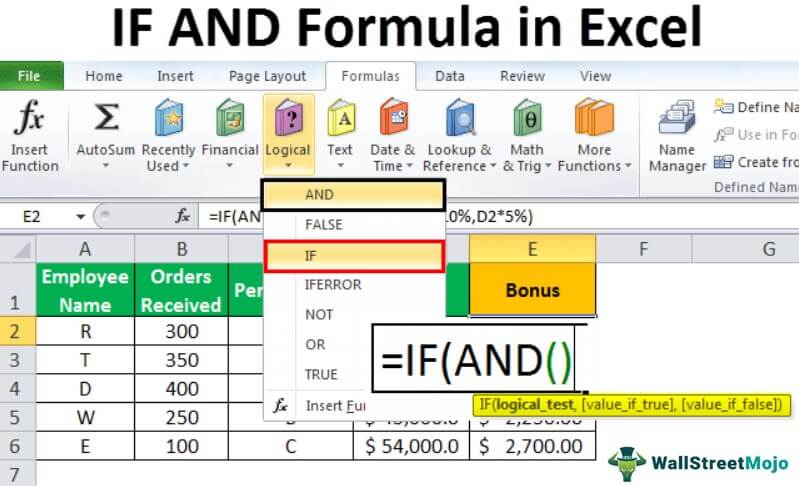
The IF function allows you to make a logical comparison between a value and what you expect by testing for a condition and returning a result if that condition is True or False.
-
=IF(Something is True, then do something, otherwise do something else)
But what if you need to test multiple conditions, where let’s say all conditions need to be True or False (AND), or only one condition needs to be True or False (OR), or if you want to check if a condition does NOT meet your criteria? All 3 functions can be used on their own, but it’s much more common to see them paired with IF functions.
Use the IF function along with AND, OR and NOT to perform multiple evaluations if conditions are True or False.
Syntax
-
IF(AND()) — IF(AND(logical1, [logical2], …), value_if_true, [value_if_false]))
-
IF(OR()) — IF(OR(logical1, [logical2], …), value_if_true, [value_if_false]))
-
IF(NOT()) — IF(NOT(logical1), value_if_true, [value_if_false]))
|
Argument name |
Description |
|
|
logical_test (required) |
The condition you want to test. |
|
|
value_if_true (required) |
The value that you want returned if the result of logical_test is TRUE. |
|
|
value_if_false (optional) |
The value that you want returned if the result of logical_test is FALSE. |
|
Here are overviews of how to structure AND, OR and NOT functions individually. When you combine each one of them with an IF statement, they read like this:
-
AND – =IF(AND(Something is True, Something else is True), Value if True, Value if False)
-
OR – =IF(OR(Something is True, Something else is True), Value if True, Value if False)
-
NOT – =IF(NOT(Something is True), Value if True, Value if False)
Examples
Following are examples of some common nested IF(AND()), IF(OR()) and IF(NOT()) statements. The AND and OR functions can support up to 255 individual conditions, but it’s not good practice to use more than a few because complex, nested formulas can get very difficult to build, test and maintain. The NOT function only takes one condition.

Here are the formulas spelled out according to their logic:
|
Formula |
Description |
|---|---|
|
=IF(AND(A2>0,B2<100),TRUE, FALSE) |
IF A2 (25) is greater than 0, AND B2 (75) is less than 100, then return TRUE, otherwise return FALSE. In this case both conditions are true, so TRUE is returned. |
|
=IF(AND(A3=»Red»,B3=»Green»),TRUE,FALSE) |
If A3 (“Blue”) = “Red”, AND B3 (“Green”) equals “Green” then return TRUE, otherwise return FALSE. In this case only the first condition is true, so FALSE is returned. |
|
=IF(OR(A4>0,B4<50),TRUE, FALSE) |
IF A4 (25) is greater than 0, OR B4 (75) is less than 50, then return TRUE, otherwise return FALSE. In this case, only the first condition is TRUE, but since OR only requires one argument to be true the formula returns TRUE. |
|
=IF(OR(A5=»Red»,B5=»Green»),TRUE,FALSE) |
IF A5 (“Blue”) equals “Red”, OR B5 (“Green”) equals “Green” then return TRUE, otherwise return FALSE. In this case, the second argument is True, so the formula returns TRUE. |
|
=IF(NOT(A6>50),TRUE,FALSE) |
IF A6 (25) is NOT greater than 50, then return TRUE, otherwise return FALSE. In this case 25 is not greater than 50, so the formula returns TRUE. |
|
=IF(NOT(A7=»Red»),TRUE,FALSE) |
IF A7 (“Blue”) is NOT equal to “Red”, then return TRUE, otherwise return FALSE. |
Note that all of the examples have a closing parenthesis after their respective conditions are entered. The remaining True/False arguments are then left as part of the outer IF statement. You can also substitute Text or Numeric values for the TRUE/FALSE values to be returned in the examples.
Here are some examples of using AND, OR and NOT to evaluate dates.

Here are the formulas spelled out according to their logic:
|
Formula |
Description |
|---|---|
|
=IF(A2>B2,TRUE,FALSE) |
IF A2 is greater than B2, return TRUE, otherwise return FALSE. 03/12/14 is greater than 01/01/14, so the formula returns TRUE. |
|
=IF(AND(A3>B2,A3<C2),TRUE,FALSE) |
IF A3 is greater than B2 AND A3 is less than C2, return TRUE, otherwise return FALSE. In this case both arguments are true, so the formula returns TRUE. |
|
=IF(OR(A4>B2,A4<B2+60),TRUE,FALSE) |
IF A4 is greater than B2 OR A4 is less than B2 + 60, return TRUE, otherwise return FALSE. In this case the first argument is true, but the second is false. Since OR only needs one of the arguments to be true, the formula returns TRUE. If you use the Evaluate Formula Wizard from the Formula tab you’ll see how Excel evaluates the formula. |
|
=IF(NOT(A5>B2),TRUE,FALSE) |
IF A5 is not greater than B2, then return TRUE, otherwise return FALSE. In this case, A5 is greater than B2, so the formula returns FALSE. |

Using AND, OR and NOT with Conditional Formatting
You can also use AND, OR and NOT to set Conditional Formatting criteria with the formula option. When you do this you can omit the IF function and use AND, OR and NOT on their own.
From the Home tab, click Conditional Formatting > New Rule. Next, select the “Use a formula to determine which cells to format” option, enter your formula and apply the format of your choice.

Using the earlier Dates example, here is what the formulas would be.

|
Formula |
Description |
|---|---|
|
=A2>B2 |
If A2 is greater than B2, format the cell, otherwise do nothing. |
|
=AND(A3>B2,A3<C2) |
If A3 is greater than B2 AND A3 is less than C2, format the cell, otherwise do nothing. |
|
=OR(A4>B2,A4<B2+60) |
If A4 is greater than B2 OR A4 is less than B2 plus 60 (days), then format the cell, otherwise do nothing. |
|
=NOT(A5>B2) |
If A5 is NOT greater than B2, format the cell, otherwise do nothing. In this case A5 is greater than B2, so the result will return FALSE. If you were to change the formula to =NOT(B2>A5) it would return TRUE and the cell would be formatted. |
Note: A common error is to enter your formula into Conditional Formatting without the equals sign (=). If you do this you’ll see that the Conditional Formatting dialog will add the equals sign and quotes to the formula — =»OR(A4>B2,A4<B2+60)», so you’ll need to remove the quotes before the formula will respond properly.
Need more help?

See also
You can always ask an expert in the Excel Tech Community or get support in the Answers community.
Learn how to use nested functions in a formula
IF function
AND function
OR function
NOT function
Overview of formulas in Excel
How to avoid broken formulas
Detect errors in formulas
Keyboard shortcuts in Excel
Logical functions (reference)
Excel functions (alphabetical)
Excel functions (by category)
IF function is undoubtedly one of the most important functions in excel. In general, IF statements give the desired intelligence to a program so that it can make decisions based on given criteria and, most importantly, decide the program flow.
In Microsoft Excel terminology, IF statements are also called «Excel IF-Then statements». IF function evaluates a boolean/logical expression and returns one value if the expression evaluates to ‘TRUE’ and another value if the expression evaluates to ‘FALSE’.
Definition of Excel IF Function
According to Microsoft Excel, IF function is defined as a formula which «checks whether a condition is met, returns one value if true and another value if false».
Syntax
Syntax of IF function in Excel is as follows:
=IF(logic_test, [value_if_true], [value_if_false])
'logic_test' (required argument) – Refers to the boolean expression or logical expression that needs to be evaluated.'value_if_true' (optional argument) – Refers to the value that will be returned by the IF function if the 'logic_test' evaluates to TRUE.'value_if_false' (optional argument) – Refers to the value that will be returned by the IF function if the 'logic_test' evaluates to FALSE.

Important Characteristics of IF Function in Excel
- To use the IF function, you need to provide the
'logic_test'or conditional statement mandatorily. - The arguments
'value_if_true'and'value_if_false'are optional, but you need to provide at least one of them. - The result of the IF statement can only be any one of the two given values (either it will be
'value_if_true'or'value_if_false'). Both values cannot be returned at the same time. - IF function throws a ‘#Name?’ error if the
'logic_test'or boolean expression you are trying to evaluate is invalid. - Nesting of IF statements is possible, but Excel only allows this to 64 levels. Nesting of IF statement means using one if statement within another.
Comparison Operators That Can Be Used With IF Statements
Following comparison operators can be used within the 'logic_test' argument of the IF function:
- = (equal to)
- <> (not equal to)
- < (less than)
- > (greater than)
- >= (greater than or equal to)
- <= (less than or equal to)
- Apart from these, you can also use any other function that returns a boolean result (either ‘true’ or ‘false’). For example – ISBLANK, ISERROR, ISEVEN, ISODD, etc
Now, let’s see some simple examples to use these comparison operators within the IF Function:
Simple Examples of Excel IF Statement
Now, let’s try to see a simple example of the Excel IF function:
Example 1: Using ‘equal to’ comparison operator within the IF function
In this example, we have a list of colors, and we aim to find the ‘Blue’ color. If we are able to find the ‘Blue’ color, then in the adjacent cell, we need to assign a ‘Yes’; otherwise, assign a ‘No’.

So, the formula would be:
=IF(A2="Blue", "No", "Yes")
This suggests that if the value present in cell A2 is ‘Blue’, then return a ‘Yes’; otherwise, return a ‘No’.
If we drag this formula down to all the rows, we will find that it returns ‘Yes’ for the cells with the value ‘Blue’ for all others; it would result in ‘No’.
Example 2: Using ‘not equal to’ comparison operator within the IF function.
Let’s take example 1, and understand how we can reverse the logic and use a ‘not equal to’ operator to construct the formula so that it still results in ‘Yes’ for ‘Blue’ color and ‘No’ for any other text.

So the formula would be:
=IF(A2<>"Blue", "No", "Yes")
This suggests that if the value at A2 is not equal to ‘Blue’, then return a ‘No’; otherwise, return a ‘Yes’.
When dragged down to all the below rows, this formula would find all the cells (from A2 to A8) where the value is not ‘Blue’ and marks a ‘No’ against them. Otherwise, it marks a ‘Yes’ in the adjacent cells.
Example 3: Using ‘less than’ operator within the IF function.
In this example, we have scores of some students, along with their names. We want to assign either «Pass» or «Fail» against each student in the result column.

Based on our criteria, the passing score is 50 or more.
For this, we can use the IF function as:
=IF(B2<50,"Fail","Pass")
This suggests that if the value at B2, i.e., 37, is less than 50, then return «Fail»; otherwise, return «Pass».
As 37 is less than 50 so the result will be «Fail».
We can drag the above-given formula for the rest of the cells below and the result would be correct.
Example 4: Using ‘greater than or equal to’ operator within the IF statement.
Let’s take example 3 and see how we can reverse the logic and use a ‘greater than or equal to’ operator to construct the formula so that it still results in ‘Pass’ for scores of 50 or more and ‘Fail’ for all the other scores.

For this, we can use the Excel IF function as:
=IF(B2>=50,"Pass","Fail")
This suggests that if the value at B2, i.e., 37 is greater than or equal to 50, then return «Pass»; otherwise, return «Fail».
As 37 not greater than or equal to 50 so the result will be «Fail».
When dragged down for the rest of the cells below, this formula would assign the correct result in the adjacent rows.
Example 5: Using ‘greater than’ operator within the IF statement.
In this example, we have a small online store that gives a discount to its customers based on the amount they spend. If a customer spends $50 or more, he is applicable for a 5% discount; otherwise, no discounts are offered.

To find whether a discount is offered or not, we can use the following excel formula:
=IF(B2>50,"5% Discount","No Discount")
This translates to – If the value at B2 cell is greater than 50, assign a text «5% Discount» otherwise, assign a text «No Discount» against the customer.
In the first case, as 23 is not greater than 50, the output will be «No Discount».
We can drag the above-given formula for the rest of the cells below are the result would be correct.
Example 6: Using ‘less than or equal to’ operator within the IF statement.
Let’s take example 5 and see how we can reverse the logic and use a ‘less than or equal to’ operator to construct the formula so that it still results in a ‘5% Discount’ for all customers whose total spend exceeds $50 and ‘No Discount’ for all the other customers.

For this, we can use the IF-then statement as:
=IF(B2<=50,"No Discount","5% Discount")
This means that if the value at B2, i.e., 23, is less than or equal to 50, then return «No Discount»; otherwise, return «5% Discount».
As 23 is less than or equal to 50 so the result will be «No Discount».
When dragged down for the rest of the cells below, this formula would assign the correct result in the adjacent rows.
Example 7: Using an Excel Logical Function within the IF formula in Excel.
In this example, let’s suppose we have a list of numbers, and we have to mark Even and Odd numbers. We can do this using the IF condition and the ISEVEN or ISODD inbuilt functions provided by Microsoft Excel.
ISEVEN function returns ‘true’ if the number passed to it is even; otherwise, it returns a ‘false’. Similarly, ISODD function return ‘true’ if the number passed to it is odd; otherwise, it returns a ‘false’.

For this, we can use the IF-then statement as:
=IF(ISEVEN(A2),"Even","Odd")
This means that – If the value at A2 cell is an even number, then the result would be «Even»; otherwise, the result would be «Odd».
Alternatively, the above logic can also be written using the ISODD function along with the IF statement as:
=IF(ISODD(A2),"Odd","Even")
This means that – If the value at A2 cell is an odd number, then the result would be «Odd»; otherwise, the result would be «Even».
Example 8: Using the Excel IF function to return another formula a result.
In this example, we have Employee Data from a company. The company comes up with a simple way to reward its loyal employees. They decide to give the employees an annual bonus based on the years spent by the employee within the organization.
Employees with experience of more than 5 years are given 10% of annual salary as a bonus whereas everyone else gets a 5% of annual salary as a bonus.

For this, the excel formula would be:
=IF(B2>5,C2*10%,C2*5%)
This means that – if the value at B2 (experience column) is greater than 5, then return a result by calculating 10% of C2 (annual salary column). However, if the logic test is evaluated to false, then return the result by calculating 5% of C2 (annual salary column)
Use Of AND & OR Functions or Logical Operators with Excel IF Statement
Excel IF Statement can also be used along with the other functions like AND, OR, NOT for analyzing complex logic. These functions (AND, OR & NOT) are called logical operators as they are used for connecting two or more logical expressions.
AND Function– AND function returns true when all the conditions inside the AND function evaluate to true. The syntax of AND Function in Excel is:
=AND(Logic1, Logic2, logic_n)
OR Function– OR function returns true when any one of the conditions inside the OR function evaluates to true. The syntax of OR Function in Excel is:
=OR(Logic1, Logic2, logic_n)
Example 9: Using the IF function along with AND Function.
In this example, we have Math and science test scores of some students, and we want to assign a ‘Pass’ or ‘Fail’ value against the students based on their scores.
Passing criteria: Students have to get more than 50 marks in Math and more than 70 marks in science to pass the test.

Based on the above conditions, the formula would be:
=IF(AND(B2>50,C2>70),"Pass","Fail")
The formula translates to – if the value at B2 (Math score) is greater than 50 and the value at C2 (Science Score) is greater than 70, then assign the value «Pass»; otherwise, assign the value «Fail».
Example 10: Using the IF function along with OR Function.
In this example, we have two test scores of some students, and we want to assign a ‘Pass’ or ‘Fail’ value against the students based on their scores.
Passing criteria: Students have to clear either one of the two tests with more than 50 marks.

Based on the above conditions, the formula would be:
=IF(OR(B2>50,C2>50),"Pass","Fail")
The formula translates to – if either the value at B2 (Test 1 score) is greater than 50, OR the value at C2 (Test 2 Score) is greater than 50, then assign the value «Pass»; otherwise, assign the value «Fail».
Recommended Reading: Excel NOT Function
Nested IF Statements
When used alone, IF formula can only result in two outcomes, i.e., True or False. But there are many cases when we want to test multiple outcomes with IF statement.
In such cases, nesting two or more IF Then statements one inside another can be convenient in writing formulas.
Syntax:
The syntax of the Nested IF Then statements is as follows:
=IF(condition_1,value_if_true_1,IF(condition_2,value_if_true_2,value_if_false_2))
'condition_1' – Refers to the first logical test or conditional expression that needs to be evaluated by the outer IF function.'value_if_true_1' – Refers to the value that will be returned by the outer IF function if the 'condition_1' evaluates to TRUE.'condition_2' – Refers to the second logical test or conditional expression that needs to be evaluated by the inner IF function.'value_if_true_2' – Refers to the value that will be returned by the inner IF function if the 'condition_2' evaluates to TRUE.'value_if_false_2' – Refers to the value that will be returned by the inner IF function if the 'condition_2' evaluates to FALSE.
The above syntax translates to this:
IF Condition1 = true THEN value_if_true1 'If Condition1 is true
ELSE IF Condition2 = true THEN value_if_true2 'Elseif Clause Condition2 is true
ELSE value_if_false2 'If both conditions are false
END IF 'End of IF Statement
As we can see, Nested formulas can quickly become complicated so, let’s try to understand how nesting of the IF statement works with an example.
Recommended Reading: VBA Select Case Statement
Example 11: Nested IF Statements
In this example, we have a list of countries and their average temperatures in degree Celsius for the month of January. Our goal is to categorize the country based on the temperature range as follows:
Criteria: Temperatures below 20 °C should be marked as «Below Room Temperature», temperatures between 20°C to 25°C should be classified as «Normal Room Temperature», whereas any temperature over 25°C should be marked as «Above Room Temperature».

Based on the above conditions, the formula would be:
=IF(B2<20,"Below Room Temperature",IF(AND(B2>=20,B2<=25),"Normal Room Temperature", "Above Room Temperature"))
The formula translates to – if the value at B2 is less than 20, then the text «Below Room Temperature» is returned from the outer IF block. However, if the value at B2 is greater than or equal to 20, then the inner IF block is evaluated.
Inside the inner IF block, the value at B2 is checked. If the value at B2 is greater than or equal to 20 and less than or equal to 25. Then the inner IF block returns the text «Normal Room Temperature».
However, if the condition inside the inner IF block also evaluates to ‘false’ that means the value at B2 is greater than 25, so the result will be «Above Room Temperature».
Recommended Reading: SWITCH Function in Excel
Partial Matching or Wildcards with IF Function
Although IF function itself doesn’t accept any wildcard characters like (* or ?) while performing the logic test, thankfully, there are ways to perform partial matching and wildcard searches with the IF function.
To perform partial matching inside the IF function, we can use the FIND (case sensitive) or SEARCH (case insensitive) functions.
Let’s have a look at this with some examples.
Example 12: Using FIND and SEARCH functions inside the IF statement
In this example, we have a list of customers, and we need to find all the customers whose last name is «Flynn». If the customer name contains the text «Flynn», then we need to assign a text «Found» against their names. Otherwise, we need to assign a text «Not Found».

For this, we can make use of the FIND function within the IF function as:
=IF(ISNUMBER(FIND("Flynn",A2)),"Found","Not Found")
Using the FIND function, we perform a case-sensitive search of the text «Flynn» within the customer name column. If the FIND function is able to find the text «Flynn», it returns a number signifying the position where it found the text.
If the number returned by the FIND function is valid, the ISNUMBER Function returns a value true. Else, it returns false. Based on the ISNUMBER function’s output, the logic test is performed and the appropriate value «Found» or «Not Found» is assigned.
Note: It should be noted that the FIND function performs a case-sensitive search.
This means in the above example if the customer name is entered in lower case (like «sean flynn» then the above function would return not found against them.
To perform a case-insensitive search, we can replace the find function with the search function, and the rest of the formula would be the same.
=IF(ISNUMBER(SEARCH("Flynn",A2)),"Found","Not Found")
Example 13: Using SEARCH function inside the Excel IF formula with wildcard operators
In this example, we have the same customer list from example 12, and we need to find all the customers whose name contains «M». If the customer name contains the alphabet «M», we need to assign a text «M Found» against their names. Otherwise, we need to assign a text «M Not Found».

For this, we can use the SEARCH function with a wildcard ‘*’ operator inside the IF function as:
=IF(ISNUMBER(SEARCH("M*",A2)),"M Found","M Not Found")
For more details on Search Function and wildcard, operators check out this article – Search Function In Excel
Some Practical Examples of using the IF function
Now, let’s have a look at some more practical examples of the Excel IF Function.
Example 14: Using Excel IF function with dates.
In this example, we have a task list along with the task due dates. Our goal is to show results based on the task due date.
If the task due date was in the past, we need to show «Was due {1,2,3..} day(s) back», if the task due date is today’s date, we need to show «Today» and similarly, if the task due date is in the future then we need to show «Due in {1,2,3..} day(s)»

In Microsoft Excel, we can do this with the help of the IF-then statement and TODAY function, as shown below:
=IF(B2=TODAY(),"Today", IF(B2>TODAY(),CONCAT("Due in ",B2-TODAY()," day(s)"), CONCAT("Was due ",TODAY()-B2," day(s) back")))
This means that – compare the date present in cell B2 if the date is equal to today’s date show the text «Today». If the date in cell B2 is not equal to today’s date, then the inner IF block checks if the date in B2 is greater than today’s date. If the date in cell B2 is greater than today’s date, that means the date is in the future, so show the text «Due in {1,2,3…} days».
However, if the date in cell B2 is not greater than today’s date, that means the date was in the past; in such a case, show the text «Was due {1,2,3..} day(s) back».
You can also go a step further and apply conditional formatting on the range and highlight all the cells with the text «Today!». This will help you to clearly see
Example 15: Use an IF function-based formula to find blank cells in excel.
In this example, we will use the IF function to find the blank cells in Microsoft Excel. We have a list of customers, and in between the list, some of the cells are blank. We aim to find the blank cells and add the text «blank call found!» against them.

We can do this with the help of the IF function along with the ISBLANK function. The ISBLANK function returns a true if the cell reference passed to it is blank. Otherwise, the ISBLANK function returns false.
Let’s see the formula –
=IF(ISBLANK(A2), "Blank cell found!"," ")
This means that – If the cell at A2 is blank, then the resultant text should be «Blank cell found!», however, if the cell at A2 is not blank, then don’t show any text.
Example 16: Use the Excel IF statement to show symbolic results (instead of textual results).
In this example, we have a list of sales employees of a company along with the number of products sold by the employees in the current month. We want to show an upward arrow symbol (↑) if the employee has done more than 50 sales and a downward arrow symbol (↓) if the employee has made less than 50 sales.

To do this, we can use the formula:
=IF(B2>50,$G$6,$G$8)
This implies – If the value at B2 is greater than 50, then, as a result, show the content in cell G6 (cell containing upward arrow) and otherwise show the content at G8 (cell containing downward arrow)
If you wonder about the ‘$’ signs used in the formula, you can check out this post – Excel Absolute References. These ‘$’ symbols are used for making excel cell references absolute.
Recommended Reading: CHOOSE Function in Excel
IFS Function In Excel:
IFS Function in Microsoft Excel is a great alternative to nested IF Statements. It is very similar to a switch statement. The IFS function evaluates multiple conditions passed to it and returns the value corresponding to the first condition that evaluates to true.
IFS function is a lot simple to write and read than nested IF statements. IFS function is available in Office 2019 and higher versions.
Syntax for IFS function:
=IFS (test1, value1, [test2, value2], ...)
'test1' (required argument) – Refers to the first logical test that needs to be evaluated.
'value1' (required argument) – Refers to the result to be returned when 'test1'evaluates to TRUE.
'test2' (optional argument) – Refers to the second logical test that needs to be evaluated
'value2' (optional argument) – Refers to the result to be returned when 'test2'evaluates to TRUE.
Example 17: Using IFS function in Excel
In this example, we have a list of students, along with their scores, and we need to assign a grade to the students based on the scores.
The grading criteria is as follows – Grade A for a score of 90 or more, Grade B for a score between 80 to 89.99, Grade C for a score between 70 to 79.99, Grade D for a score between 60 to 69.99, Grade E for a score between 60 to 59.99, Grade F for a score lower than 50.

Let’s see how easily write such a complicated formula with the IFS function:
=IFS(B2 >= 90,"A",B2 >= 80,"B",B2 >= 70,"C",B2 >= 60,"D",B2 >= 50,"E",B2 < 50,"F")
This implies that – If B2 is greater than or equal to 90, return A. Else if B2 is greater than or equal to 80, return B. Else if B2 is greater than or equal to 70, return C. Else if B2 is greater than or equal to 60, return D. Else if B2 is greater than or equal to 50, return E. Else if B2 is less than 50, return F.
If you would try to write the same formula using nested IF statements, see how long and complicated it becomes:
=IF(B2 >= 90,"A",IF(B2 >= 80, "B",IF(B2 >= 70, "C",IF(B2 >= 60, "D",IF(B2 >= 50, "E",IF(B2 < 50, "F"))))))
So, this was all about the IF function in excel. If you want to learn more about IF function, I would recommend you to go through this article – VBA IF Statement With Examples
IF AND Excel Formula
The IF AND excel formula is the combination of two different logical functions often nested together that enables the user to evaluate multiple conditions using AND functions. Based on the output of the AND function, the IF function returns either the “true” or “false” value, respectively.
- The IF formula in ExcelIF function in Excel evaluates whether a given condition is met and returns a value depending on whether the result is “true” or “false”. It is a conditional function of Excel, which returns the result based on the fulfillment or non-fulfillment of the given criteria.
read more is used to test and compare the conditions expressed with the expected value. It is used to test a single criterion. - The logical AND formula is used to test multiple criteria. It returns “true” if all the conditions mentioned are satisfied, or else returns “false.” It tests more than one criterion and accordingly returns an output. It can also be used along with the IF formula to return the desired result.
Table of contents
- IF AND Excel Formula
- Syntax
- How to Use IF AND Excel Statement?
- Example #1
- Example #2
- Example #3
- The Characteristics of IF AND function
- Frequently Asked Questions
- Recommended Articles
Syntax
The IF AND formula can be applied as follows:
“=IF(AND (Condition 1,Condition 2,…),Value _if _True,Value _if _False)”
You are free to use this image on your website, templates, etc, Please provide us with an attribution linkArticle Link to be Hyperlinked
For eg:
Source: IF AND in Excel (wallstreetmojo.com)
How to Use IF AND Excel Statement?
You can download this IF AND Formula Excel Template here – IF AND Formula Excel Template
Let us understand the usage of the IF AND formula with the help of some examples mentioned below:
Example #1
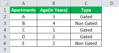
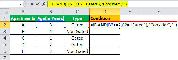
The table given below provides a list of apartments along with their age (in years) and type of society. Now we need to perform a comparative analysis for the apartments based on the age of the building and the type of society.
Here, we use the combination of less than equal (<=) to operator and the equal to (=) text functions in the condition to be demonstrated for IF AND function.
- The IF AND formula used to perform the analysis is stated as follows:
“=IF(AND(B2<=2,C2=“Gated”),“Consider”, “”)”
- The succeeding image shows the IF AND condition applied to perform the evaluation.
- Press “Enter” to get the answer.
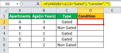
- Drag the formula to find the results for all the apartments.
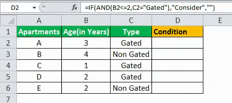
The results in the cell D of the above table shows that the IF AND formula will be performing one among the following:
- If both the arguments entered in the AND function is “true,” then the IF function will return that apartment to be “Consider.”
- If either of the arguments in the AND functionThe AND function in Excel is classified as a logical function; it returns TRUE if the specified conditions are met, otherwise it returns FALSE.read more is “false” or both the arguments entered are “false,” then the IF function will return a blank string.
The IF AND formula can also perform calculations based on whether the AND function returns “true” or “false,” apart from returning only the predefined text strings.
We will understand this concept with the help of the below-mentioned example.
Example #2
The given data tableA data table in excel is a type of what-if analysis tool that allows you to compare variables and see how they impact the result and overall data. It can be found under the data tab in the what-if analysis section.read more has the list of employee name along with their orders received, performance, and salaries. Calculate the employee hike (or bonus) based on two parameters–the number of orders received and performance.
The criteria to calculate the bonus is as follows.
- The number of orders received is greater than or equal to 200, and the performance is equal to “A.”
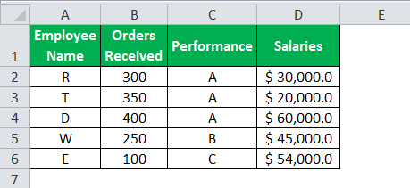
- The IF AND formula will be,
“=IF(AND(B2>=200,C2= “A”),D2*10%,D2*5%)”
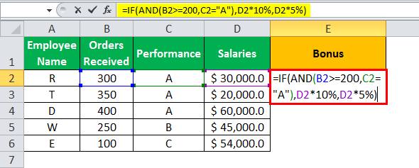
- Press “Enter” to get the final output. The bonus appears in cell E2.
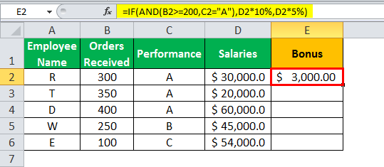
- Drag the formula to find the bonus of all employees.
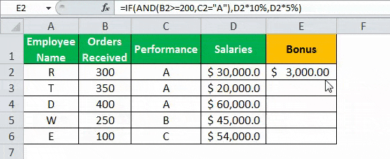
Based on these results, the IF formula does the following evaluation:
- If both the conditions are satisfied, the AND function returns “true,” then the bonus received is calculated as salary multiplied by 10%.
- If either one or both the conditions are found to be “false” by the AND function, then the bonus is calculated as salary multiplied by 5%.
Examples 1 and 2 have only two criteria to test and evaluate. Using multiple arguments or conditions to test them for “true” or “false” is also allowed.
Example #3
Let us evaluate multiple criteria and use AND function.
A table with five stocks and their parameter details including financial ratiosFinancial ratios are indications of a company’s financial performance. There are several forms of financial ratios that indicate the company’s results, financial risks, and operational efficiency, such as the liquidity ratio, asset turnover ratio, operating profitability ratios, business risk ratios, financial risk ratio, stability ratios, and so on.read more, such as ROCEReturn on Capital Employed (ROCE) is a metric that analyses how effectively a company uses its capital and, as a result, indicates long-term profitability. ROCE=EBIT/Capital Employed.read more, ROEReturn on Equity (ROE) represents financial performance of a company. It is calculated as the net income divided by the shareholders equity. ROE signifies the efficiency in which the company is using assets to make profit.read more, Debt to equityThe debt to equity ratio is a representation of the company’s capital structure that determines the proportion of external liabilities to the shareholders’ equity. It helps the investors determine the organization’s leverage position and risk level. read more, and PE ratioThe price to earnings (PE) ratio measures the relative value of the corporate stocks, i.e., whether it is undervalued or overvalued. It is calculated as the proportion of the current price per share to the earnings per share. read more is provided (shown in the below table). Using this data lets us test the condition to invest in suitable stocks. That is, using the parameters, let us analyze the stocks to derive the best investment horizonThe term «investment horizon» refers to the amount of time an investor is expected to hold an investment portfolio or a security before selling it. Depending on the need for funds and risk appetite, the investor may invest for a few days or hours to a few years or decades.read more, which is important for growth.
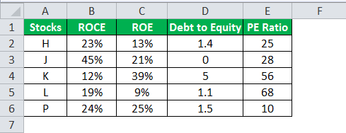
The following syntax is used where the conditions are applied to arrive at the result (shown in the below table).
“=IF(AND(B2>18%,C2>20%,D2<2,E2<30%),“Invest”,“”)”

- Press “Enter” to get the final output (Investment Criteria) of the above formula.

- Drag the formula to find the Investment Criteria.
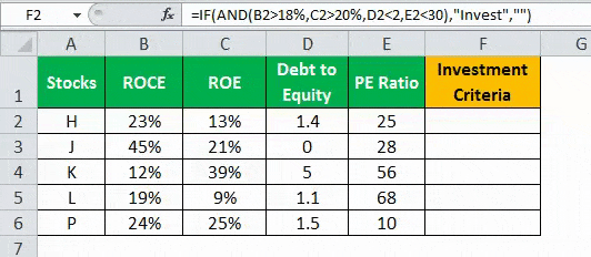
In the above data table, the AND function tests for the parameters using the operators. The resulting output generated by the IF formula is as follows:
- If all the four criteria mentioned in the AND function are tested and satisfied, then the IF function returns the “Invest” text string.
- If either one or more among the four conditions or all the four conditions fail to satisfy the AND function, then the IF function returns empty strings (“”).
The Characteristics of IF AND function
- The IF AND function does not differentiate between case-insensitive texts.
- The AND function can be used to evaluate up to 255 conditions for “true” or “false,” and the total formula length does not exceed 8192 characters.
- Text values or blank cells are given as an argument to test the conditions in AND function.
- The AND formula will return “#VALUE!” if there is no logical output found while evaluating the conditions.
- IF AND excel statement is a combination of two logical functions that tests and evaluates multiple conditions.
- The output of the AND function is based on, whether the IF function will return the value “true” or “false,” respectively.
- IF function is used to test a single criterion whereas, the AND function is used to test multiple criteria.
- The syntax of the IF AND formula is:
“=IF(AND (Condition 1,Condition 2,…),Value _if _True,Value _if _False)”
- The IF AND formula also performs a calculation based on whether the AND function is “true” or “false” apart from returning only the predefined text strings.
Frequently Asked Questions
1. How to use IF AND function in Excel?
The IF AND excel statement is the two logical functions often nested together.
Syntax:
“=IF(AND(Condition1,Condition2, value_if_true,vaue_if_false)”
The IF formula is used to test and compare the conditions expressed, along with the expected value. It provides the desired result if the condition is either “true” or “false.”
The AND formula is used to test multiple criteria. It returns “true” if all the given conditions are satisfied, or else returns “false.”
2. What is the IF AND function in Excel?
IF AND formula is applied as the combination of the two logical functions that enable the user to evaluate the multiple conditions. Based on the output of the AND function, the IF function returns the output “true” or “false.”
3. How to combine IF and AND functions in Excel?
To combine IF and AND functions, you need to replace the “condition_test” argument in the IF function with AND function.
“=IF(condition_test, value_if_true,vaue_if_false)”
“=IF(AND(Condition1,Condition2, value_if_true,vaue_if_false)”
In AND function we can use multiple conditions.
Recommended Articles
This has been a guide to IF AND function in Excel. Here we discuss how to use IF Formula combined with AND function along with examples and downloadable templates. You may also look at these useful functions in Excel –
- IF EXCEL FunctionIF function in Excel evaluates whether a given condition is met and returns a value depending on whether the result is “true” or “false”. It is a conditional function of Excel, which returns the result based on the fulfillment or non-fulfillment of the given criteria.
read more - Average IF Function
- SUMIF with Multiple CriteriaThe SUMIF (SUM+IF) with multiple criteria sums the cell values based on the conditions provided. The criteria are based on dates, numbers, and text. The SUMIF function works with a single criterion, while the SUMIFS function works with multiple criteria in excel.read more
- Nested If ConditionIn Excel, nested if function means using another logical or conditional function with the if function to test multiple conditions. For example, if there are two conditions to be tested, we can use the logical functions AND or OR depending on the situation, or we can use the other conditional functions to test even more ifs inside a single if.read more
Purpose
Test multiple conditions with AND
Return value
TRUE if all arguments evaluate TRUE; FALSE if not
Usage notes
The AND function is used to check more than one logical condition at the same time, up to 255 conditions, supplied as arguments. Each argument (logical1, logical2, etc.) must be an expression that returns TRUE or FALSE or a value that can be evaluated as TRUE or FALSE. The arguments provided to the AND function can be constants, cell references, arrays, or logical expressions.
The purpose of the AND function is to evaluate more than one logical test at the same time and return TRUE only if all results are TRUE. For example, if A1 contains the number 50, then:
=AND(A1>0,A1>10,A1<100) // returns TRUE
=AND(A1>0,A1>10,A1<30) // returns FALSE
The AND function will evaluate all values supplied and return TRUE only if all values evaluate to TRUE. If any value evaluates to FALSE, the AND function will return FALSE. Note: Excel will evaluate any number except zero (0) as TRUE.
Both the AND function and the OR function will aggregate results to a single value. This means they can’t be used in array operations that need to deliver an array of results. To work around this limitation, you can use Boolean logic. For more information, see: Array formulas with AND and OR logic.
Examples
To test if the value in A1 is greater than 0 and less than 5, you can use AND like this:
=AND(A1>0,A1<5)
You can embed the AND function inside the IF function. Using the above example, you can supply AND as the logical_test for the IF function like so:
=IF(AND(A1>0,A1<5), "Approved", "Denied")
This formula will return «Approved» only if the value in A1 is greater than 0 and less than 5.
You can combine the AND function with the OR function. The formula below returns TRUE when A1 > 100 and B1 is «complete» or «pending»:
=AND(A1>100,OR(B1="complete",B1="pending"))
See below for many more examples of how the AND function can be used.
Notes
- The AND function is not case-sensitive.
- The AND function does not support wildcards.
- Text values or empty cells supplied as arguments are ignored.
- The AND function will return #VALUE if no logical values are found or created during evaluation.
Brief syntax lesson
Cells(Row, Column) identifies a cell. Row must be an integer between 1 and the maximum for version of Excel you are using. Column must be a identifier (for example: «A», «IV», «XFD») or a number (for example: 1, 256, 16384)
.Cells(Row, Column) identifies a cell within a sheet identified in a earlier With statement:
With ActiveSheet
  :
  .Cells(Row,Column)
  :
End With
If you omit the dot, Cells(Row,Column) is within the active worksheet. So wsh = ActiveWorkbook wsh.Range is not strictly necessary. However, I always use a With statement so I do not wonder which sheet I meant when I return to my code in six months time. So, I would write:
With ActiveSheet
  :
  .Range.
  :
End With
Actually, I would not write the above unless I really did want the code to work on the active sheet. What if the user has the wrong sheet active when they started the macro. I would write:
With Sheets("xxxx")
  :
  .Range.
  :
End With
because my code only works on sheet xxxx.
Cells(Row,Column) identifies a cell. Cells(Row,Column).xxxx identifies a property of the cell. Value is a property. Value is the default property so you can usually omit it and the compiler will know what you mean. But in certain situations the compiler can be confused so the advice to include the .Value is good.
Cells(Row,Column) like "*Miami*" will give True if the cell is «Miami», «South Miami», «Miami, North» or anything similar.
Cells(Row,Column).Value = "Miami" will give True if the cell is exactly equal to «Miami». «MIAMI» for example will give False. If you want to accept MIAMI, use the lower case function:
Lcase(Cells(Row,Column).Value) = "miami"
My suggestions
Your sample code keeps changing as you try different suggestions which I find confusing. You were using Cells(Row,Column) <> "Miami" when I started typing this.
Use
If Cells(i, "A").Value like "*Miami*" And Cells(i, "D").Value like "*Florida*" Then
  Cells(i, "C").Value = "BA"
if you want to accept, for example, «South Miami» and «Miami, North».
Use
If Cells(i, "A").Value = "Miami" And Cells(i, "D").Value like "Florida" Then
  Cells(i, "C").Value = "BA"
if you want to accept, exactly, «Miami» and «Florida».
Use
If Lcase(Cells(i, "A").Value) = "miami" And _
   Lcase(Cells(i, "D").Value) = "florida" Then
  Cells(i, "C").Value = "BA"
if you don’t care about case.