Using and function in excel with if

The IF function allows you to make a logical comparison between a value and what you expect by testing for a condition and returning a result if that condition is True or False.

=IF(Something is True, then do something, otherwise do something else)

But what if you need to test multiple conditions, where let’s say all conditions need to be True or False (AND), or only one condition needs to be True or False (OR), or if you want to check if a condition does NOT meet your criteria? All 3 functions can be used on their own, but it’s much more common to see them paired with IF functions.

Use the IF function along with AND, OR and NOT to perform multiple evaluations if conditions are True or False.

Syntax

IF(AND()) — IF(AND(logical1, [logical2], …), value_if_true, [value_if_false]))
IF(OR()) — IF(OR(logical1, [logical2], …), value_if_true, [value_if_false]))
IF(NOT()) — IF(NOT(logical1), value_if_true, [value_if_false]))


Argument name	Description
logical_test (required)	The condition you want to test.
value_if_true (required)	The value that you want returned if the result of logical_test is TRUE.

value_if_false (optional)	The value that you want returned if the result of logical_test is FALSE.

Here are overviews of how to structure AND, OR and NOT functions individually. When you combine each one of them with an IF statement, they read like this:

AND – =IF(AND(Something is True, Something else is True), Value if True, Value if False)
OR – =IF(OR(Something is True, Something else is True), Value if True, Value if False)
NOT – =IF(NOT(Something is True), Value if True, Value if False)

Examples

Following are examples of some common nested IF(AND()), IF(OR()) and IF(NOT()) statements. The AND and OR functions can support up to 255 individual conditions, but it’s not good practice to use more than a few because complex, nested formulas can get very difficult to build, test and maintain. The NOT function only takes one condition.

Here are the formulas spelled out according to their logic:

Formula	Description
=IF(AND(A2>0,B2<100),TRUE, FALSE)	IF A2 (25) is greater than 0, AND B2 (75) is less than 100, then return TRUE, otherwise return FALSE. In this case both conditions are true, so TRUE is returned.
=IF(AND(A3=»Red»,B3=»Green»),TRUE,FALSE)	If A3 (“Blue”) = “Red”, AND B3 (“Green”) equals “Green” then return TRUE, otherwise return FALSE. In this case only the first condition is true, so FALSE is returned.
=IF(OR(A4>0,B4<50),TRUE, FALSE)	IF A4 (25) is greater than 0, OR B4 (75) is less than 50, then return TRUE, otherwise return FALSE. In this case, only the first condition is TRUE, but since OR only requires one argument to be true the formula returns TRUE.
=IF(OR(A5=»Red»,B5=»Green»),TRUE,FALSE)	IF A5 (“Blue”) equals “Red”, OR B5 (“Green”) equals “Green” then return TRUE, otherwise return FALSE. In this case, the second argument is True, so the formula returns TRUE.
=IF(NOT(A6>50),TRUE,FALSE)	IF A6 (25) is NOT greater than 50, then return TRUE, otherwise return FALSE. In this case 25 is not greater than 50, so the formula returns TRUE.
=IF(NOT(A7=»Red»),TRUE,FALSE)	IF A7 (“Blue”) is NOT equal to “Red”, then return TRUE, otherwise return FALSE.

Note that all of the examples have a closing parenthesis after their respective conditions are entered. The remaining True/False arguments are then left as part of the outer IF statement. You can also substitute Text or Numeric values for the TRUE/FALSE values to be returned in the examples.

Here are some examples of using AND, OR and NOT to evaluate dates.

Here are the formulas spelled out according to their logic:

Formula	Description
=IF(A2>B2,TRUE,FALSE)	IF A2 is greater than B2, return TRUE, otherwise return FALSE. 03/12/14 is greater than 01/01/14, so the formula returns TRUE.
=IF(AND(A3>B2,A3<C2),TRUE,FALSE)	IF A3 is greater than B2 AND A3 is less than C2, return TRUE, otherwise return FALSE. In this case both arguments are true, so the formula returns TRUE.
=IF(OR(A4>B2,A4<B2+60),TRUE,FALSE)	IF A4 is greater than B2 OR A4 is less than B2 + 60, return TRUE, otherwise return FALSE. In this case the first argument is true, but the second is false. Since OR only needs one of the arguments to be true, the formula returns TRUE. If you use the Evaluate Formula Wizard from the Formula tab you’ll see how Excel evaluates the formula.
=IF(NOT(A5>B2),TRUE,FALSE)	IF A5 is not greater than B2, then return TRUE, otherwise return FALSE. In this case, A5 is greater than B2, so the formula returns FALSE.

Using AND, OR and NOT with Conditional Formatting

You can also use AND, OR and NOT to set Conditional Formatting criteria with the formula option. When you do this you can omit the IF function and use AND, OR and NOT on their own.

From the Home tab, click Conditional Formatting > New Rule. Next, select the “Use a formula to determine which cells to format” option, enter your formula and apply the format of your choice.

Using the earlier Dates example, here is what the formulas would be.

Formula	Description
=A2>B2	If A2 is greater than B2, format the cell, otherwise do nothing.
=AND(A3>B2,A3<C2)	If A3 is greater than B2 AND A3 is less than C2, format the cell, otherwise do nothing.
=OR(A4>B2,A4<B2+60)	If A4 is greater than B2 OR A4 is less than B2 plus 60 (days), then format the cell, otherwise do nothing.
=NOT(A5>B2)	If A5 is NOT greater than B2, format the cell, otherwise do nothing. In this case A5 is greater than B2, so the result will return FALSE. If you were to change the formula to =NOT(B2>A5) it would return TRUE and the cell would be formatted.

Note: A common error is to enter your formula into Conditional Formatting without the equals sign (=). If you do this you’ll see that the Conditional Formatting dialog will add the equals sign and quotes to the formula — =»OR(A4>B2,A4<B2+60)», so you’ll need to remove the quotes before the formula will respond properly.

Need more help?

Quick Intro

Both of these functions are useful but by using them jointly, you can solve some real-life problems. Here is a quick intro for both.

IF Function – To test a condition and return a specific value if that condition is true or another specific value if that condition is false.
AND Function – To test multiple conditions. If all the conditions are true then it will return true and if any of the conditions are false then it will return false.

Why is this Important?

You can test more than one condition with the IF function.
It will return a specific value if all the conditions are true.
Or, it will return another specific value if any of the conditions are false.

How do IF and AND Functions Work?

To combine IF and AND functions you have to just replace the logical_test argument in the IF function with AND function. By using AND function you can specify more than one condition.

how to combine if and and functions replace logical test

Now AND function will test your all conditions here. If all the conditions are true then AND function will return true and the IF function will return the value which you have specified for true.

And, if any of the conditions is false then AND function will return false, and the IF function will return the value which you have specified for false. Let me show you a real-life example.

Examples

Here I have a marks sheet of students. And, I want to add some remarks to the sheet.

how to combine if and and functions table to add status

If a student is passed both of the subjects with 40 marks or above, the status should be “Pass”. And, if a student has less than 40 marks in both of the subjects or even in one subject, the status should be “Fail”. The formula will be.

=IF(AND(B2>=40,C2>=40),"Pass","Fail")

how to combine if and and functions insert formula

In the above formula, if there is a value 40 or greater than in any of the cells (B2 & C2) AND function will return true, and IF will return the value “Pass”. That means if a student passed both of the subjects then he/she will pass.

But, if both cells have a value lower than 40 then AND will return false, and IF will return the value “Fail”. If a student is failed in any of the subjects he/she will fail.

Download Sample File

Ready

And, if you want to Get Smarter than Your Colleagues check out these FREE COURSES to Learn Excel, Excel Skills, and Excel Tips and Tricks.

Источник

IF AND Excel Formula

The IF AND excel formula is the combination of two different logical functions often nested together that enables the user to evaluate multiple conditions using AND functions. Based on the output of the AND function, the IF function returns either the “true” or “false” value, respectively.

The IF formula in ExcelIF function in Excel evaluates whether a given condition is met and returns a value depending on whether the result is “true” or “false”. It is a conditional function of Excel, which returns the result based on the fulfillment or non-fulfillment of the given criteria.
read more is used to test and compare the conditions expressed with the expected value. It is used to test a single criterion.
The logical AND formula is used to test multiple criteria. It returns “true” if all the conditions mentioned are satisfied, or else returns “false.” It tests more than one criterion and accordingly returns an output. It can also be used along with the IF formula to return the desired result.

IF AND Excel Formula
- Syntax
- How to Use IF AND Excel Statement?
  - Example #1
  - Example #2
  - Example #3
- The Characteristics of IF AND function
- Frequently Asked Questions
- Recommended Articles

Syntax

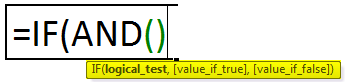
The IF AND formula can be applied as follows:

“=IF(AND (Condition 1,Condition 2,…),Value _if _True,Value _if _False)”

You are free to use this image on your website, templates, etc, Please provide us with an attribution linkArticle Link to be Hyperlinked
For eg:
Source: IF AND in Excel (wallstreetmojo.com)

How to Use IF AND Excel Statement?

You can download this IF AND Formula Excel Template here – IF AND Formula Excel Template

Let us understand the usage of the IF AND formula with the help of some examples mentioned below:

Example #1

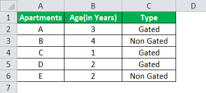
The table given below provides a list of apartments along with their age (in years) and type of society. Now we need to perform a comparative analysis for the apartments based on the age of the building and the type of society.

Here, we use the combination of less than equal (<=) to operator and the equal to (=) text functions in the condition to be demonstrated for IF AND function.

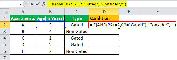
The IF AND formula used to perform the analysis is stated as follows:

“=IF(AND(B2<=2,C2=“Gated”),“Consider”, “”)”

The succeeding image shows the IF AND condition applied to perform the evaluation.

Press “Enter” to get the answer.

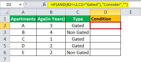
Drag the formula to find the results for all the apartments.

The results in the cell D of the above table shows that the IF AND formula will be performing one among the following:

If both the arguments entered in the AND function is “true,” then the IF function will return that apartment to be “Consider.”
If either of the arguments in the AND functionThe AND function in Excel is classified as a logical function; it returns TRUE if the specified conditions are met, otherwise it returns FALSE.read more is “false” or both the arguments entered are “false,” then the IF function will return a blank string.

The IF AND formula can also perform calculations based on whether the AND function returns “true” or “false,” apart from returning only the predefined text strings.

We will understand this concept with the help of the below-mentioned example.

Example #2

The given data tableA data table in excel is a type of what-if analysis tool that allows you to compare variables and see how they impact the result and overall data. It can be found under the data tab in the what-if analysis section.read more has the list of employee name along with their orders received, performance, and salaries. Calculate the employee hike (or bonus) based on two parameters–the number of orders received and performance.

The criteria to calculate the bonus is as follows.

The number of orders received is greater than or equal to 200, and the performance is equal to “A.”

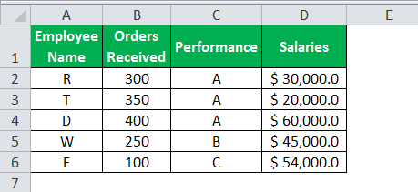
The IF AND formula will be,

“=IF(AND(B2>=200,C2= “A”),D2*10%,D2*5%)”

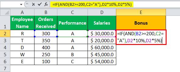
Press “Enter” to get the final output. The bonus appears in cell E2.

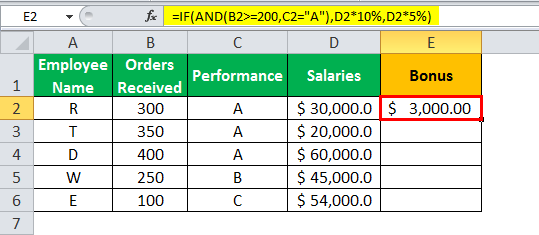
Drag the formula to find the bonus of all employees.

Based on these results, the IF formula does the following evaluation:

If both the conditions are satisfied, the AND function returns “true,” then the bonus received is calculated as salary multiplied by 10%.
If either one or both the conditions are found to be “false” by the AND function, then the bonus is calculated as salary multiplied by 5%.

Examples 1 and 2 have only two criteria to test and evaluate. Using multiple arguments or conditions to test them for “true” or “false” is also allowed.

Example #3

Let us evaluate multiple criteria and use AND function.

A table with five stocks and their parameter details including financial ratiosFinancial ratios are indications of a company’s financial performance. There are several forms of financial ratios that indicate the company’s results, financial risks, and operational efficiency, such as the liquidity ratio, asset turnover ratio, operating profitability ratios, business risk ratios, financial risk ratio, stability ratios, and so on.read more, such as ROCEReturn on Capital Employed (ROCE) is a metric that analyses how effectively a company uses its capital and, as a result, indicates long-term profitability. ROCE=EBIT/Capital Employed.read more, ROEReturn on Equity (ROE) represents financial performance of a company. It is calculated as the net income divided by the shareholders equity. ROE signifies the efficiency in which the company is using assets to make profit.read more, Debt to equityThe debt to equity ratio is a representation of the company’s capital structure that determines the proportion of external liabilities to the shareholders’ equity. It helps the investors determine the organization’s leverage position and risk level. read more, and PE ratioThe price to earnings (PE) ratio measures the relative value of the corporate stocks, i.e., whether it is undervalued or overvalued. It is calculated as the proportion of the current price per share to the earnings per share. read more is provided (shown in the below table). Using this data lets us test the condition to invest in suitable stocks. That is, using the parameters, let us analyze the stocks to derive the best investment horizonThe term «investment horizon» refers to the amount of time an investor is expected to hold an investment portfolio or a security before selling it. Depending on the need for funds and risk appetite, the investor may invest for a few days or hours to a few years or decades.read more, which is important for growth.

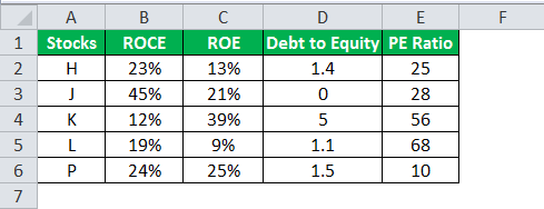
The following syntax is used where the conditions are applied to arrive at the result (shown in the below table).

“=IF(AND(B2>18%,C2>20%,D2<2,E2<30%),“Invest”,“”)”

Press “Enter” to get the final output (Investment Criteria) of the above formula.

Drag the formula to find the Investment Criteria.

In the above data table, the AND function tests for the parameters using the operators. The resulting output generated by the IF formula is as follows:

If all the four criteria mentioned in the AND function are tested and satisfied, then the IF function returns the “Invest” text string.
If either one or more among the four conditions or all the four conditions fail to satisfy the AND function, then the IF function returns empty strings (“”).

The Characteristics of IF AND function

The IF AND function does not differentiate between case-insensitive texts.
The AND function can be used to evaluate up to 255 conditions for “true” or “false,” and the total formula length does not exceed 8192 characters.
Text values or blank cells are given as an argument to test the conditions in AND function.
The AND formula will return “#VALUE!” if there is no logical output found while evaluating the conditions.

IF AND excel statement is a combination of two logical functions that tests and evaluates multiple conditions.
The output of the AND function is based on, whether the IF function will return the value “true” or “false,” respectively.
IF function is used to test a single criterion whereas, the AND function is used to test multiple criteria.
The syntax of the IF AND formula is:

“=IF(AND (Condition 1,Condition 2,…),Value _if _True,Value _if _False)”

The IF AND formula also performs a calculation based on whether the AND function is “true” or “false” apart from returning only the predefined text strings.

Frequently Asked Questions

1. How to use IF AND function in Excel?

The IF AND excel statement is the two logical functions often nested together.

Syntax:
“=IF(AND(Condition1,Condition2, value_if_true,vaue_if_false)”

The IF formula is used to test and compare the conditions expressed, along with the expected value. It provides the desired result if the condition is either “true” or “false.”

The AND formula is used to test multiple criteria. It returns “true” if all the given conditions are satisfied, or else returns “false.”

2. What is the IF AND function in Excel?

IF AND formula is applied as the combination of the two logical functions that enable the user to evaluate the multiple conditions. Based on the output of the AND function, the IF function returns the output “true” or “false.”

3. How to combine IF and AND functions in Excel?

To combine IF and AND functions, you need to replace the “condition_test” argument in the IF function with AND function.

“=IF(condition_test, value_if_true,vaue_if_false)”

“=IF(AND(Condition1,Condition2, value_if_true,vaue_if_false)”

In AND function we can use multiple conditions.

Description

The IF function can be combined with the AND function to allow you to test for multiple conditions. When using the AND function, all conditions within the AND function must be TRUE for the condition to be met.

If you want to follow along with this tutorial, download the example spreadsheet.

Download Example

Syntax

The syntax for the IF function with the AND function in Microsoft Excel is:

IF( AND( condition1, [condition2], ... ), value_if_true, [value_if_false] )

Parameters or Arguments

condition1, condition2, …: The conditions to test. There must be at least 1 condition entered in the AND function and you can have up to 30 conditions.
value_if_true: It is the value that is returned if all conditions in the AND function evaluate to TRUE.
value_if_false: Optional. It is the value that is returned if any of the conditions in the AND function evaluate to FALSE.

Returns

Returns value_if_true when all of the conditions in the AND function are TRUE.
Returns value_if_false when any of the conditions in the AND function are FALSE.
Returns FALSE if the value_if_false parameter is omitted and any of the conditions in the AND function are FALSE.

Applies To

Excel for Office 365, Excel 2019, Excel 2016, Excel 2013, Excel 2011 for Mac, Excel 2010, Excel 2007, Excel 2003, Excel XP, Excel 2000

Example (as Worksheet Function)

Let’s explore how to use the IF function with the AND function in Microsoft Excel.

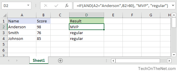
Based on the spreadsheet above, you can combine the IF function with the AND function as follows:

=IF(AND(A2="Anderson",B2>80), "MVP", "regular")
Result: "MVP"

=IF(AND(B2>=80,B2<=100), "Great Score", "Not Bad")
Result: "Great Score"

=IF(AND(B3>=80,B3<=100), "Great Score", "Not Bad")
Result: "Not Bad"

=IF(AND(A2="Anderson",A3="Smith",A4="Johnson"), 100, 50)
Result: 100

=IF(AND(A2="Anderson",A3="Smith",A4="Parker"), 100, 50)
Result: 50

In the examples above, all conditions within the AND function must be TRUE for the condition to be met.

Источник

In this tutorial, we will learn about the IF function in Excel. Along with IF, the AND and OR functions are important formulas too. A nested IF simply means multiple IF functions in a single syntax.

Introducing IF Function in Excel

Let’s get started with this easy guide to using the IF function and all its related functions in Microsoft Excel, step-by-step with supporting images and examples.

1. IF Function

To learn to use the IF function, we will take an example of a mark list of students below.

Our goal is to find out which student has passed or failed and what are their grades. Of course, it would be a tedious task to find out pass or fail results and grades for each student in this list.

To ease our task, we have IF functions for that matter. The IF function will automatically identify if a student has passed or failed based on the criteria you provide to it.

It will automatically mark a student as “Pass” if he/she has scored above the minimum pass mark and mark a student as “Fail” if he/she has scored below the minimum pass mark.

The IF function automatically assigns the appropriate grades to students based on their marks if you command it.

Here is a glimpse of how the IF function helps you out with assigning grades and marking “Pass” or “Fail”.

Steps to use IF function in Excel

We have allotted certain grades and marked them as Pass or Fail to students based on the percentages they have secured in their exams, with the help of the IF function.

1. Using the IF function in Excel to identify passed/failed students

Let’s learn how we can use the IF formula to achieve this. We will use the same example. We take the minimum passing percentage as 34%.

Find out the percentage of total marks of every student.
Create a new column named “Pass/Fail”.
In the blank cell below the title, type the IF formula as follows next.
Type =IF( and select the first student’s percentage and type >=34.
Put a comma and move to the next argument named [value_if_true]. This means you’re being asked to put a value to be displayed if the above condition is true. Remember these arguments are case sensitive.
Once you have put a comma, type “Pass”.
Put a comma and move to the next argument named [value_if_false] to display a value when the above condition is false. This field is optional in most cases but we need a false value because it is a mark list.
Close the bracket and hit ENTER.

You can see that the formula is displaying “Pass” for the first student because she has secured above 34%.

Double-click or drag the cell from the right corner below to autofill the formula to all the students below.

Recommended read: How to Autofill in Excel?

2. Nested IF Function

Now, let us start assigning grades to all students.

We are going to be using multiple IF functions in a single syntax this time to provide multiple criteria to the IF function. This is called Nested IF in Excel.

However, there is no specific function named “Nested IF” in Excel, it is simply that this behavior has been given a name i.e., Nested IF.

Before we proceed further, we need to first make a table that displays a grading class for each grade. Here is an example below.

Create a new column named “Grade”.
Type the IF function in a blank cell below the title as follows.
Type =IF( and now type AE118>=85,”A”,IF(AE118>=70,”B”,IF(AE118>=55,”C”,IF(AE118>=34,”D”,IF(AE118<=33,”Fail”.

Note that AE118 is our cell address for the first student’s percentage. It will be different in your case. Refer to the image above to make sense of the formula.
The formula simply states- if percentage marks are above and equal to 85 then give “A”, if percentage marks are above and equal to 70 then give “B”, and so on and so forth. For the last condition, we have applied the condition- if the marks are less than or equal to 33 then give “Fail”.
For the last IF statement, you can either put the result as “Fail” or “E” as you like.
Now, note that we will close the formula with 5 brackets for this example as we have used a total of 5 IF formulas.

Hit ENTER to complete the formula.

You can now see that the formula has been applied to the first entry and the result is B because the student has secured 72.5% which is less than 75%. This means the nested Ifs are working correctly.

Now drag the cell from the lower right corner to autofill the formula to the rest of the entries.

You can see that we now have grades and pass/fail markings for every student on the list successfully.

3. IF with AND in Excel

Let us learn the IF formula with the AND function in a single syntax with a minor example.

When you have two or more distinct conditions to be used together, you can use the IF function with AND in Excel.

While nested IFs will also work, using AND function will save your time as it is shorter to type. So, let’s get started.

Our goal is to identify currencies with revenues greater than 20,000 and less than 50,000 and mark them as “Good”.

Type =IF(AND( because we are using the IF with AND function.
Select the first cell under Revenue, and type >20000.
Put a comma and select the first cell under Revenue again and type <50000.
Now, close the bracket to complete the AND function. We’re still working on the IF function so do not put two brackets.
We come back to the IF function as soon as we close the AND function. Now put the values to be displayed if the condition is true or false.
Put a comma to move to the argument [value_if_true] and type “Good”.
You can provide a result in the [value_if_false] argument, but it is completely optional. If nothing is provided then the cells will display FALSE if the condition is false. But if you want the cells to remain blank simply put “” (two double quotation marks) in this argument.
Close the bracket to complete the IF function as well.

This is how the syntax should look like before pressing ENTER.

Hit ENTER to view results and drag the cell down to autofill the formula to the rest of the cells.

There are only two such cells for which the condition is true and the result is being displayed as “Good” for them and the rest of the cells are blank. This means the formula is working correctly.

4. IF with OR in Excel

Using the OR function with the IF function will give results for either of the conditions that are true.

Type =IF(OR(.
Select the first cell under Revenue and type >=20000.
Put a comma and select the first cell under Revenue again and type <=50000.
Now, close the bracket to complete the OR function. We’re still working on the IF function so do not put two brackets.
Coming back to the IF function, we now put the values to be displayed if the condition is true or false.
Put a comma to move to the argument [value_if_true] and type “Flag”.
Put a comma to move to the argument [value_if_false] and type “”.

This is how the syntax should look like before pressing ENTER.

Close the bracket to complete the OR function and hit ENTER.
Drag the cell below to get the results for the rest.

The formula is true for all entries and so it is displaying “Flag” for all of them. This is because all the values are either lower than 50,000 or greater than 20,000.

Conclusion

This was all about IF functions and other related functions to the IF function that are AND and OR functions.

Reference: ExcelJet

Источник

Examples

Using AND, OR and NOT with Conditional Formatting

Need more help?

See also

Quick Intro

Why is this Important?

How do IF and AND Functions Work?

Examples

Download Sample File

IF AND Excel Formula

Table of contents

Syntax

How to Use IF AND Excel Statement?

Example #1

Example #2

Example #3

The Characteristics of IF AND function

Frequently Asked Questions

Recommended Articles

Description

Syntax

Parameters or Arguments

Returns

Applies To

Example (as Worksheet Function)

Introducing IF Function in Excel

1. IF Function

Steps to use IF function in Excel

1. Using the IF function in Excel to identify passed/failed students

2. Nested IF Function

3. IF with AND in Excel

4. IF with OR in Excel

Conclusion