
Excel for Microsoft 365 Excel for Microsoft 365 for Mac Excel for the web Excel 2021 Excel 2021 for Mac Excel 2019 Excel 2019 for Mac Excel 2016 Excel 2016 for Mac Excel 2013 Excel 2010 Excel 2007 More…Less
Although Excel includes a multitude of built-in worksheet functions, chances are it doesn’t have a function for every type of calculation you perform. The designers of Excel couldn’t possibly anticipate every user’s calculation needs. Instead, Excel provides you with the ability to create custom functions, which are explained in this article.
Custom functions, like macros, use the Visual Basic for Applications (VBA) programming language. They differ from macros in two significant ways. First, they use Function procedures instead of Sub procedures. That is, they start with a Function statement instead of a Sub statement and end with End Function instead of End Sub. Second, they perform calculations instead of taking actions. Certain kinds of statements, such as statements that select and format ranges, are excluded from custom functions. In this article, you’ll learn how to create and use custom functions. To create functions and macros, you work with the Visual Basic Editor (VBE), which opens in a new window separate from Excel.
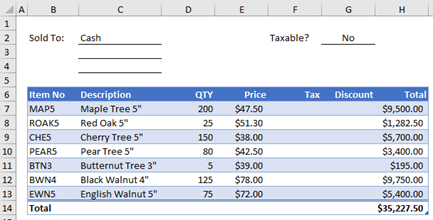
Suppose your company offers a quantity discount of 10 percent on the sale of a product, provided the order is for more than 100 units. In the following paragraphs, we’ll demonstrate a function to calculate this discount.
The example below shows an order form that lists each item, quantity, price, discount (if any), and the resulting extended price.
To create a custom DISCOUNT function in this workbook, follow these steps:
-
Press Alt+F11 to open the Visual Basic Editor (on the Mac, press FN+ALT+F11), and then click Insert > Module. A new module window appears on the right-hand side of the Visual Basic Editor.
-
Copy and paste the following code to the new module.
Function DISCOUNT(quantity, price)
   If quantity >=100 Then
     DISCOUNT = quantity * price * 0.1
   Else
     DISCOUNT = 0
   End If

 DISCOUNT = Application.Round(Discount, 2)
End Function
Note: To make your code more readable, you can use the Tab key to indent lines. The indentation is for your benefit only, and is optional, as the code will run with or without it. After you type an indented line, the Visual Basic Editor assumes your next line will be similarly indented. To move out (that is, to the left) one tab character, press Shift+Tab.
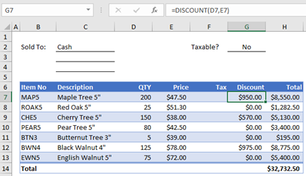
Now you’re ready to use the new DISCOUNT function. Close the Visual Basic Editor, select cell G7, and type the following:
=DISCOUNT(D7,E7)
Excel calculates the 10 percent discount on 200 units at $47.50 per unit and returns $950.00.
In the first line of your VBA code, Function DISCOUNT(quantity, price), you indicated that the DISCOUNT function requires two arguments, quantity and price. When you call the function in a worksheet cell, you must include those two arguments. In the formula =DISCOUNT(D7,E7), D7 is the quantity argument, and E7 is the price argument. Now you can copy the DISCOUNT formula to G8:G13 to get the results shown below.
Let’s consider how Excel interprets this function procedure. When you press Enter, Excel looks for the name DISCOUNT in the current workbook and finds that it is a custom function in a VBA module. The argument names enclosed in parentheses, quantity and price, are placeholders for the values on which the calculation of the discount is based.
The If statement in the following block of code examines the quantity argument and determines whether the number of items sold is greater than or equal to 100:
If quantity >= 100 Then
 DISCOUNT = quantity * price * 0.1
Else
 DISCOUNT = 0
End If
If the number of items sold is greater than or equal to 100, VBA executes the following statement, which multiplies the quantity value by the price value and then multiplies the result by 0.1:
Discount = quantity * price * 0.1
The result is stored as the variable Discount. A VBA statement that stores a value in a variable is called an assignment statement, because it evaluates the expression on the right side of the equal sign and assigns the result to the variable name on the left. Because the variable Discount has the same name as the function procedure, the value stored in the variable is returned to the worksheet formula that called the DISCOUNT function.
If quantity is less than 100, VBA executes the following statement:
Discount = 0
Finally, the following statement rounds the value assigned to the Discount variable to two decimal places:
Discount = Application.Round(Discount, 2)
VBA has no ROUND function, but Excel does. Therefore, to use ROUND in this statement, you tell VBA to look for the Round method (function) in the Application object (Excel). You do that by adding the word Application before the word Round. Use this syntax whenever you need to access an Excel function from a VBA module.
A custom function must start with a Function statement and end with an End Function statement. In addition to the function name, the Function statement usually specifies one or more arguments. You can, however, create a function with no arguments. Excel includes several built-in functions—RAND and NOW, for example—that don’t use arguments.
Following the Function statement, a function procedure includes one or more VBA statements that make decisions and perform calculations using the arguments passed to the function. Finally, somewhere in the function procedure, you must include a statement that assigns a value to a variable with the same name as the function. This value is returned to the formula that calls the function.
The number of VBA keywords you can use in custom functions is smaller than the number you can use in macros. Custom functions are not allowed to do anything other than return a value to a formula in a worksheet, or to an expression used in another VBA macro or function. For example, custom functions cannot resize windows, edit a formula in a cell, or change the font, color, or pattern options for the text in a cell. If you include “action” code of this kind in a function procedure, the function returns the #VALUE! error.
The one action a function procedure can do (apart from performing calculations) is display a dialog box. You can use an InputBox statement in a custom function as a means of getting input from the user executing the function. You can use a MsgBox statement as a means of conveying information to the user. You can also use custom dialog boxes, or UserForms, but that’s a subject beyond the scope of this introduction.
Even simple macros and custom functions can be difficult to read. You can make them easier to understand by typing explanatory text in the form of comments. You add comments by preceding the explanatory text with an apostrophe. For example, the following example shows the DISCOUNT function with comments. Adding comments like these makes it easier for you or others to maintain your VBA code as time passes. If you need to make a change to the code in the future, you’ll have an easier time understanding what you did originally.
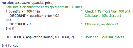
An apostrophe tells Excel to ignore everything to the right on the same line, so you can create comments either on lines by themselves or on the right side of lines containing VBA code. You might begin a relatively long block of code with a comment that explains its overall purpose and then use inline comments to document individual statements.
Another way to document your macros and custom functions is to give them descriptive names. For example, rather than name a macro Labels, you could name it MonthLabels to describe more specifically the purpose the macro serves. Using descriptive names for macros and custom functions is especially helpful when you’ve created many procedures, particularly if you create procedures that have similar but not identical purposes.
How you document your macros and custom functions is a matter of personal preference. What’s important is to adopt some method of documentation, and use it consistently.
To use a custom function, the workbook containing the module in which you created the function must be open. If that workbook is not open, you get a #NAME? error when you try to use the function. If you reference the function in a different workbook, you must precede the function name with the name of the workbook in which the function resides. For example, if you create a function called DISCOUNT in a workbook called Personal.xlsb and you call that function from another workbook, you must type =personal.xlsb!discount(), not simply =discount().
You can save yourself some keystrokes (and possible typing errors) by selecting your custom functions from the Insert Function dialog box. Your custom functions appear in the User Defined category:
An easier way to make your custom functions available at all times is to store them in a separate workbook and then save that workbook as an add-in. You can then make the add-in available whenever you run Excel. Here’s how to do this:
-
After you have created the functions you need, click File > Save As.
In Excel 2007, click the Microsoft Office Button, and click Save As
-
In the Save As dialog box, open the Save As Type drop-down list, and select Excel Add-In. Save the workbook under a recognizable name, such as MyFunctions, in the AddIns folder. The Save As dialog box will propose that folder, so all you need to do is accept the default location.
-
After you have saved the workbook, click File > Excel Options.
In Excel 2007, click the Microsoft Office Button, and click Excel Options.
-
In the Excel Options dialog box, click the Add-Ins category.
-
In the Manage drop-down list, select Excel Add-Ins. Then click the Go button.
-
In the Add-Ins dialog box, select the check box beside the name you used to save your workbook, as shown below.

-
After you have created the functions you need, click File > Save As.
-
In the Save As dialog box, open the Save As Type drop-down list, and select Excel Add-In. Save the workbook under a recognizable name, such as MyFunctions.
-
After you have saved the workbook, click Tools > Excel Add-Ins.
-
In the Add-Ins dialog box, select the Browse button to find your add-in, click Open, then check the box beside your Add-In in the Add-Ins Available box.
After you follow these steps, your custom functions will be available each time you run Excel. If you want to add to your function library, return to the Visual Basic Editor. If you look in the Visual Basic Editor Project Explorer under a VBAProject heading, you will see a module named after your add-in file. Your add-in will have the extension .xlam.
Double-clicking that module in the Project Explorer causes the Visual Basic Editor to display your function code. To add a new function, position your insertion point after the End Function statement that terminates the last function in the Code window, and begin typing. You can create as many functions as you need in this manner, and they will always be available in the User Defined category in the Insert Function dialog box.
This content was originally authored by Mark Dodge and Craig Stinson as part of their book Microsoft Office Excel 2007 Inside Out. It has since been updated to apply to newer versions of Excel as well.
Need more help?
You can always ask an expert in the Excel Tech Community or get support in the Answers community.
Need more help?
Skip to content
В решении многих задач обычные функции Excel не всегда могут помочь. Если существующих функций недостаточно, Excel позволяет добавить новые настраиваемые пользовательские функции (UDF). Они делают вашу работу легче.
Мы расскажем, как можно их создать, какие они бывают и как использовать их, чтобы ваша работа стала проще. Узнайте, как записать и использовать пользовательские функции, которые многие называют макросами..
- Что такое пользовательская функция
- Для чего ее используют?
- Как создать пользовательскую функцию в VBA?
- Как использовать пользовательскую функцию в формуле?
- Какие бывают типы пользовательских функций
Что такое пользовательская функция в Excel?
На момент написания этой статьи Excel предлагает вам более 450 различных функций. С их помощью вы можете выполнять множество различных операций. Но разработчики Microsoft Excel не могли предвидеть все задачи, которые нам нужно решать. Думаю, что многие из вас встречались с этими проблемами:
- не все данные могут быть обработаны стандартными функциями (например, даты до 1900 года).
- формулы могут быть весьма длинными и сложными. Их невозможно запомнить, трудно понять и сложно изменить для решения новой задачи.
- Не все задачи могут быть решены при помощи стандартных функций Excel (в частности, нельзя извлечь интернет-адрес из гиперссылки).
- Невозможно автоматизировать часто повторяющиеся стандартные операции (импорт данных из бухгалтерской программы на лист Excel, форматирование дат и чисел, удаление лишних колонок).
Как можно решить эти проблемы?
- Для очень сложных формул многие пользователи создают архив рабочих книг с примерами. Они копируют оттуда нужную формулу и применяют ее в своей таблице.
- Создание макросов VBA.
- Создание пользовательских функций при помощи редактора VBA.
Хотя первые два варианта кажутся вам знакомыми, третий может вызвать некоторую путаницу. Итак, давайте подробнее рассмотрим настраиваемые функции в Excel и решим, стоит ли их использовать.
Пользовательская функция – это настраиваемый код, который принимает исходные данные, производит вычисление и возвращает желаемый результат.
Исходными данными могут быть числа, текст, даты, логические значения, массивы. Результатом вычислений может быть значение любого типа, с которым работает Excel, или массив таких значений.
Другими словами, пользовательская функция – это своего рода модернизация стандартных функций Excel. Вы можете использовать ее, когда возможностей обычных функций недостаточно. Основное ее назначение – дополнить и расширить возможности Excel, выполнить действия, которые невозможны со стандартными возможностями.
Существует несколько способов создания собственных функций:
- при помощи Visual Basic for Applications (VBA). Этот способ описывается в данной статье.
- с использованием замечательной функции LAMBDA, которая появилась в Office365.
- при помощи Office Scripts. На момент написания этой статьи они доступны в Excel Online в подписке на Office365.
Посмотрите на скриншот ниже, чтобы увидеть разницу между двумя способами извлечения чисел — с использованием формулы и пользовательской функции ExtractNumber().

Даже если вы сохранили эту огромную формулу в своем архиве, вам нужно ее найти, скопировать и вставить, а затем аккуратно поправить все ссылки на ячейки. Согласитесь, это потребует затрат времени, да и ошибки не исключены.
А на ввод функции вы потратите всего несколько секунд.
Для чего можно использовать?
Вы можете использовать настраиваемую функцию одним из следующих способов:
- В формуле, где она может брать исходные данные из вашего рабочего листа и возвращать рассчитанное значение или массив значений.
- Как часть кода макроса VBA или другой пользовательской функции.
- В формулах условного форматирования.
- Для хранения констант и списков данных.
Для чего нельзя использовать пользовательские функции:
- Любого изменения другой ячейки, кроме той, в которую она записана,
- Изменения имени рабочего листа,
- Копирования листов рабочей книги,
- Поиска и замены значений,
- Изменения форматирования ячейки, шрифта, фона, границ, включения и отключения линий сетки,
- Вызова и выполнения макроса VBA, если его выполнение нарушит перечисленные выше ограничения. Если вы используете строку кода, который не может быть выполнен, вы можете получить ошибку RUNTIME ERROR либо просто одну из стандартных ошибок (например, #ЗНАЧЕН!).
Как создать пользовательскую функцию в VBA?
Прежде всего, необходимо открыть редактор Visual Basic (сокращенно — VBE). Обратите внимание, что он открывается в новом окне. Окно Excel при этом не закрывается.
Самый простой способ открыть VBE — использовать комбинацию клавиш. Это быстро и всегда доступно. Нет необходимости настраивать ленту или панель инструментов быстрого доступа. Нажмите Alt + F11 на клавиатуре, чтобы открыть VBE. И снова нажмите Alt + F11, когда редактор открыт, чтобы вернуться назад в окно Excel.

После открытия VBE вам нужно добавить новый модуль. В него вы будете записывать ваш код. Щелкните правой кнопкой мыши на панели проекта VBA слева и выберите «Insert», затем появившемся справа окне — “Module”.
Справа появится пустое окно модуля, в котором вы и будете создавать свою функцию.
Прежде чем начать, напомним правила, по которым создается функция.
- Пользовательская функция всегда начинается с оператора Function и заканчивается инструкцией End Function.
- После оператора Function указывают имя функции. Это название, которое вы создаете и присваиваете, чтобы вы могли идентифицировать и использовать ее позже. Оно не должно содержать пробелов. Если вы хотите разделять слова, используйте подчеркивания. Например, Count_Words.
- Кроме того, это имя также не может совпадать с именами стандартных функций Excel. Если вы сделаете это, то всегда будет выполняться стандартная функция.
- Имя пользовательской функции не может совпадать с адресами ячеек на листе. Например, имя ABC1234 невозможно присвоить.
- Настоятельно рекомендуется давать описательные имена. Тогда вы можете легко выбрать нужное из длинного списка функций. Например, имя CountWords позволяет легко понять, что она делает, и при необходимости применить ее для подсчета слов.
- Далее в скобках обычно перечисляют аргументы. Это те данные, с которыми она будет работать. Может быть один или несколько аргументов. Если у вас несколько аргументов, их нужно перечислить через запятую.
- После этого обычно объявляются переменные, которые использует пользовательская функция. Указывается тип этих переменных – число, дата, текст, массив.
- Если операторы, которые вы используете внутри вашей функции, не используют никакие аргументы (например, NOW (СЕЙЧАС), TODAY (СЕГОДНЯ) или RAND (СЛЧИС)), то вы можете создать функцию без аргументов. Также аргументы не нужны, если вы используете функцию для хранения констант (например, числа Пи).
- Затем записывают несколько операторов VBA, которые выполняют вычисления с использованием переданных аргументов.
- В конце вы должны вставить оператор, который присваивает итоговое значение переменной с тем же именем, что и имя функции. Это значение возвращается в формулу, из которой была вызвана пользовательская функция.
- Записанный вами код может включать комментарии. Они помогут вам не забыть назначение функции и отдельных ее операторов. Если вы в будущем захотите внести какие-то изменения, комментарии будут вам очень полезны. Комментарий всегда начинается с апострофа (‘). Апостроф указывает Excel игнорировать всё, что записано после него, и до конца строки.
Теперь давайте попробуем создать вашу первую собственную формулу. Для начала мы создаем код, который будет подсчитывать количество слов в диапазоне ячеек.
Для этого в окно модуля вставим этот код:
Function CountWords(NumRange As Range) As Long
Dim rCell As Range, lCount As Long
    For Each rCell In NumRange
        lCount = lCount + _
          Len(WorksheetFunction.Trim(rCell)) - Len(Replace(WorksheetFunction.Trim(rCell), " ", "")) + 1
    Next rCell
CountWords = lCount
End Function
Я думаю, здесь могут потребоваться некоторые пояснения.
Код функции всегда начинается с пользовательской процедуры Function. В процедуре Function мы делаем описание новой функции.
В начале мы должны записать ее имя: CountWords.
Затем в скобках указываем, какие исходные данные она будет использовать. NumRange As Range означает, что аргументом будет диапазон значений. Сюда нужно передать только один аргумент — диапазон ячеек, в котором будет происходить подсчёт.
As Long указывает, что результат выполнения функции CountWords будет целым числом.
Во второй строке кода мы объявляем переменные.
Оператор Dim объявляет переменные:
rCell — переменная диапазона ячеек, в котором мы будем подсчитывать слова.
lCount — переменная целое число, в которой будет записано число слов.
Цикл For Each… Next предназначен для выполнения вычислений по отношению к каждому элементу из группы элементов (нашего диапазона ячеек). Этот оператор цикла применяется, когда неизвестно количество элементов в группе. Начинаем с первого элемента, затем берем следующий и так повторяем до самого последнего значения. Цикл повторяется столько раз, сколько ячеек имеется во входном диапазоне.
Внутри этого цикла с значением каждой ячейки выполняется операция, которая вычисляет количество слов:
Len(WorksheetFunction.Trim(rCell)) — Len(Replace(WorksheetFunction.Trim(rCell), » «, «»)) + 1
Как видите, это обычная формула Excel, которая использует стандартные средства работы с текстом: LEN, TRIM и REPLACE. Это английские названия знакомых нам русскоязычных ДЛСТР, СЖПРОБЕЛЫ и ЗАМЕНИТЬ. Вместо адреса ячейки рабочего листа используем переменную диапазона rCell. То есть, для каждой ячейки диапазона мы последовательно считаем количество слов в ней.
Подсчитанные числа суммируются и сохраняются в переменной lCount:
lCount = lCount + Len(WorksheetFunction.Trim(rCell)) — Len(Replace(WorksheetFunction.Trim(rCell), » «, «»)) + 1
Когда цикл будет завершен, значение переменной присваивается функции.
CountWords = lCount
Функция возвращает в ячейку рабочего листа значение этой переменной, то есть общее количество слов.
Именно эта строка кода гарантирует, что функция вернет значение lCount обратно в ячейку, из которой она была вызвана.
Закрываем наш код с помощью «End Function».
Как видите, не очень сложно.
Сохраните вашу работу. Для этого просто нажмите кнопку “Save” на ленте VB редактора.
После этого вы можете закрыть окно редактора. Для этого можно использовать комбинацию клавиш Alt+Q. Или просто вернитесь на лист Excel, нажав Alt+F11.
Вы можете сравнить работу с пользовательской функцией CountWords и подсчет количества слов в диапазоне при помощи формул.
Как использовать пользовательскую функцию в формуле?
Когда вы создали пользовательскую, она становится доступной так же, как и другие стандартные функции Excel. Сейчас мы узнаем, как создавать с ее помощью собственные формулы.
Чтобы использовать ее, у вас есть две возможности.
Первый способ. Нажмите кнопку fx в строке формул. Среди появившихся категорий вы увидите новую группу — Определённые пользователем. И внутри этой категории вы можете увидеть нашу новую пользовательскую функцию CountWords.

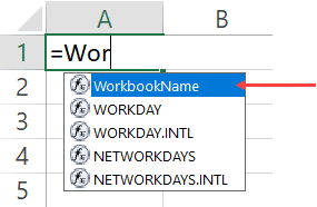
Второй способ. Вы можете просто записать эту функцию в ячейку так же, как вы это делаете обычно. Когда вы начинаете вводить имя, Excel покажет вам имя пользовательской в списке соответствующих функций. В приведенном ниже примере, когда я ввел = cou , Excel показал мне список подходящих функций, среди которых вы видите и CountWords.

Можно посчитать этой же функцией и количество слов в диапазоне. Запишите в ячейку С3:
=CountWords(A2:A5)
Нажмите Enter.
Мы только что указали функцию и установили диапазон, и вот результат подсчета: 14 слов.
Для сравнения в C1 я записал формулу массива, при помощи которой мы также можем подсчитать количество слов в диапазоне.

Как видите, результаты одинаковы. Только использовать CountWords() гораздо проще и быстрее.
Различные типы пользовательских функций с использованием VBA.
Теперь мы познакомимся с разными типами пользовательских функций в зависимости от используемых ими аргументов и результатов, которые они возвращают.
Без аргументов.
В Excel есть несколько стандартных функций, которые не требуют аргументов (например, СЛЧИС , СЕГОДНЯ , СЕЧАС). Например, СЛЧИС возвращает случайное число от 0 до 1. СЕГОДНЯ вернет текущую дату. Вам не нужно передавать им какие-либо значения.
Вы можете создать такую функцию и в VBA.
Ниже приведен код, который запишет в ячейку имя вашего рабочего листа.
Function SheetName() as String
    Application.Volatile
    SheetName = Application.Caller.Worksheet.Name
End Function
Или же можно использовать такой код:
SheetName = ActiveSheet.NameОбратите внимание, что в скобках после имени нет ни одного аргумента. Здесь не требуется никаких аргументов, так как результат, который нужно вернуть, не зависит от каких-либо значений в вашем рабочем файле.
Приведенный выше код определяет результат функции как тип данных String (поскольку желаемый результат — это имя файла, которое является текстом). Если вы не укажете тип данных, то Excel будет определять его самостоятельно.
С одним аргументом.
Создадим простую функцию, которая работает с одним аргументом, то есть с одной ячейкой. Наша задача – извлечь из текстовой строки последнее слово.
Function ReturnLastWord(The_Text As String)
Dim stLastWord As String
'Extracts the LAST word from a text string
    stLastWord = StrReverse(The_Text)
    stLastWord = Left(stLastWord, InStr(1, stLastWord, " ", vbTextCompare))
    ReturnLastWord = StrReverse(Trim(stLastWord))
End Function
Аргумент The_Text — это значение выбранной ячейки. Указываем, что это должно быть текстовое значение (As String).
Оператор StrReverse возвращает текст с обратным порядком следования знаков. Далее InStr определяет позицию первого пробела. При помощи Left получаем все знаки заканчивая первым пробелом. Затем удаляем пробелы при помощи Trim. Вновь меняем порядок следования символов при помощи StrReverse. Получаем последнее слово из текста.
Поскольку эта функция принимает значение ячейки, нам не нужно использовать здесь Application.Volatile. Как только аргумент изменится, функция автоматически обновится.
Использование массива в качестве аргумента.
Многие функции Excel используют массивы значений как аргументы. Вспомните функции СУММ, СУММЕСЛИ, СУММПРОИЗВ.
Мы уже рассмотрели эту ситуацию выше, когда учились создавать пользовательскую функцию для подсчета количества слов в диапазоне ячеек.
Приведённый ниже код создает функцию, которая суммирует все чётные числа в указанном диапазоне ячеек.
Function SumEven(NumRange as Range)
 Dim RngCell As Range
 For Each RngCell In NumRange
 If IsNumeric(RngCell.Value) Then
 If RngCell.Value Mod 2 = 0 Then
 Result = Result + RngCell.Value
 End If
 End If
 Next RngCell
 SumEven = Result
 End Function
Аргумент NumRange указан как Range. Это означает, что функция будет использовать массив исходных данных. Необходимо отметить, что можно использовать также тип переменной Variant. Это выглядит как
Function SumEven(NumRange as Variant)Тип Variant обеспечивает «безразмерный» контейнер для хранения данных. Такая переменная может хранить данные любого из допустимых в VBA типов, включая числовые значения, текст, даты и массивы. Более того, одна и та же такая переменная в одной и той же программе в разные моменты может хранить данные различных типов. Excel самостоятельно будет определять, какие данные передаются в функцию.
В коде есть цикл For Each … Next, который берет каждую ячейку и проверяет, есть ли в ней число. Если это не так, то ничего не происходит, и он переходит к следующей ячейке. Если найдено число, он проверяет, четное оно или нет (с помощью функции MOD).
Все чётные числа суммируются в переменной Result.
Когда цикл будет закончен, значение Result присваивается переменной SumEven и передаётся функции.
С несколькими аргументами.
Большинство функций Excel имеет несколько аргументов. Не являются исключением и пользовательские функции. Поэтому так важно уметь создавать собственные функции с несколькими аргументами.
В приведенном ниже коде создается функция, которая выбирает максимальное число в заданном интервале.
Она имеет 3 аргумента: диапазон значений, нижняя граница числового интервала, верхняя граница интервала.
Function GetMaxBetween(rngCells As Range, MinNum, MaxNum)
Dim NumRange As Range
Dim vMax
Dim arrNums()
Dim i As Integer
ReDim arrNums(rngCells.Count)
    For Each NumRange In rngCells
     vMax = NumRange
        Select Case vMax
           Case MinNum + 0.01 To MaxNum - 0.01
              arrNums(i) = vMax
              i = i + 1
           Case Else
               GetMaxBetween = 0
           End Select
    Next NumRange
    GetMaxBetween = WorksheetFunction.Max(arrNums)
End Function
Здесь мы используем три аргумента. Первый из них — rngCells As Range. Это диапазон ячеек, в которых нужно искать максимальное значение. Второй и третий аргумент (MinNum, MaxNum) указаны без объявления типа. Это означает, что по умолчанию к ним будет применён тип данных Variant. В VBA используется 6 различных числовых типов данных. Указывать только один из них — это значит ограничить применение функции. Поэтому более целесообразно, если Excel сам определит тип числовых данных.
Цикл For Each … Next последовательно просматривает все значения в выбранном диапазоне. Числа, которые находятся в интервале от максимального до минимального значения, записываются в специальный массив arrNums. При помощи стандартного оператора MAX в этом массиве находим наибольшее число.
С обязательными и необязательными аргументами.
Чтобы понять, что такое необязательный аргумент, вспомните функцию ВПР (VLOOKUP). Её четвертый аргумент [range_lookup] является необязательным. Если вы не укажете один из обязательных аргументов, получите ошибку. Но если вы пропустите необязательный аргумент, всё будет работать.
Но необязательные аргументы не бесполезны. Они позволяют вам выбирать вариант расчётов.
Например, в функции ВПР, если вы не укажете четвертый аргумент, будет выполнен приблизительный поиск. Если вы укажете его как ЛОЖЬ (или 0), то будет найдено точное совпадение.
Если в вашей пользовательской функции есть хотя бы один обязательный аргумент, то он должен быть записан в начале. Только после него могут идти необязательные.
Чтобы сделать аргумент необязательным, вам просто нужно добавить «Optional» перед ним.
Теперь давайте посмотрим, как создать функцию в VBA с необязательными аргументами.
Function GetText(textCell As Range, Optional CaseText = False) As String
Dim StringLength As Integer
Dim Result As String
StringLength = Len(textCell)
For i = 1 To StringLength
If Not (IsNumeric(Mid(textCell, i, 1))) Then Result = Result & Mid(textCell, i, 1)
Next i
If CaseText = True Then Result = UCase(Result)
GetText = Result
End Function
Этот код извлекает текст из ячейки. Optional CaseText = False означает, что аргумент CaseText необязательный. По умолчанию его значение установлено FALSE.
Если необязательный аргумент CaseText имеет значение TRUE, то возвращается результат в верхнем регистре. Если необязательный аргумент FALSE или опущен, результат остается как есть, без изменения регистра символов.
Думаю, что у вас возник вопрос: «Могут ли в пользовательской функции быть только необязательные аргументы?». Ответ смотрите ниже.
Только с необязательным аргументом.
Насколько мне известно, нет встроенной функции Excel, которая имеет только необязательные аргументы. Здесь я могу ошибаться, но я не могу припомнить ни одной такой.
Но при создании пользовательской такое возможно.
Перед вами функция, которая записывает в ячейку имя пользователя.
Function UserName(Optional Uppercase As Variant)
    If IsMissing(Uppercase) Then Uppercase = False
    UserName = Application.UserName
    If Uppercase Then UserName = UCase(UserName)
End Function
Как видите, здесь есть только один аргумент Uppercase, и он не обязательный.
Если аргумент равен FALSE или опущен, то имя пользователя возвращается без каких-либо изменений. Если же аргумент TRUE, то имя возвращается в символах верхнего регистра (с помощью VBA-оператора Ucase). Обратите внимание на вторую строку кода. Она содержит VBA-функцию IsMissing, которая определяет наличие аргумента. Если аргумент отсутствует, оператор присваивает переменной Uppercase значение FALSE.
Можно предложить и другой вариант этой функции.
Function UserName(Optional Uppercase As Variant)
    If IsMissing(Uppercase) Then Uppercase = False
    UserName = Application.UserName
    If Uppercase Then UserName = UCase(UserName)
End Function
В этом случае необязательный аргумент имеет значение по умолчанию FALSE. Если функция будет введена без аргументов, то значение FALSE будет использовано по умолчанию и имя пользователя будет получено без изменения регистра символов. Если будет введено любое значение кроме нуля, то все символы будут преобразованы в верхний регистр.
Возвращаемое значение — массив.
В VBA имеется весьма полезная функция — Array. Она возвращает значение с типом данных Variant, которое представляет собой массив (т.е. несколько значений).
Пользовательские функции, которые возвращают массив, весьма полезны при хранении массивов значений. Например, Months() вернёт массив названий месяцев:
Function Months() As Variant
Months = Array("Январь", "Февраль", "Март", "Апрель", "Май", "Июнь", _
"Июль", "Август", "Сентябрь", "Октябрь", "Ноябрь", "Декабрь")
End Function
Обратите внимание, что функция выводит данные в строке, по горизонтали.

В Office365 и выше можно вводить как обычную формулу, в более ранних версиях – как формулу массива.
А если необходим вертикальный массив значений?
Мы уже говорили ранее, что созданные нами функции можно использовать в формулах Excel вместе со стандартными.
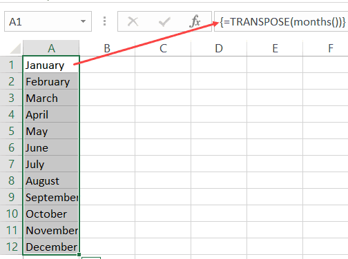
Используем Months() как аргумент функции ТРАНСП:
=ТРАНСП(Months())
![]()
Как можно использовать пользовательские функции с массивом данных? Можно применять их для ввода данных в таблицу, как показано на рисунке выше. К примеру, в отчёте о продажах не нужно вручную писать названия месяцев.
Можно получить название месяца по его номеру. Например, в ячейке A1 записан номер месяца. Тогда название месяца можно получить при помощи формулы
=ИНДЕКС(Months();1;A1)
Альтернативный вариант этой формулы:
=ИНДЕКС( {«Январь»; «Февраль»; «Март»; «Апрель»; «Май»; «Июнь»; «Июль»; «Август»; «Сентябрь»; «Октябрь»; «Ноябрь»; «Декабрь»};1;A1)
Согласитесь, написанная нами функция делает формулу Excel значительно проще.
Эта статья откроет серию материалов о пользовательских функциях. Если мне удалось убедить вас, что это стоит использовать или вы хотели бы попробовать что-то новое в Excel, следите за обновлениями;)
 Сумма по цвету и подсчёт по цвету в Excel — В этой статье вы узнаете, как посчитать ячейки по цвету и получить сумму по цвету ячеек в Excel. Эти решения работают как для окрашенных вручную, так и с условным форматированием. Если…
  Проверка данных с помощью регулярных выражений — В этом руководстве показано, как выполнять проверку данных в Excel с помощью регулярных выражений и пользовательской функции RegexMatch. Когда дело доходит до ограничения пользовательского ввода на листах Excel, проверка данных очень полезна. Хотите… Поиск и замена в Excel с помощью регулярных выражений — В этом руководстве показано, как быстро добавить пользовательскую функцию в свои рабочие книги, чтобы вы могли использовать регулярные выражения для замены текстовых строк в Excel. Когда дело доходит до замены… Как извлечь строку из текста при помощи регулярных выражений — В этом руководстве вы узнаете, как использовать регулярные выражения в Excel для поиска и извлечения части текста, соответствующего заданному шаблону. Microsoft Excel предоставляет ряд функций для извлечения текста из ячеек. Эти функции…
  4 способа отладки пользовательской функции — Как правильно создавать пользовательские функции и где нужно размещать их код, мы подробно рассмотрели ранее в этой статье. Чтобы решить проблемы при создании пользовательской функции, вам скорее всего придется выполнить…
Excel allows you to create custom functions using VBA, called «User Defined Functions» (UDFs) that can be used the same way you would use SUM() or other built-in Excel functions. They can be especially useful for advanced mathematics or special text manipulation or date calculations prior to 1900. Many Excel add-ins provide large collections of specialized functions.
This article will help you get started creating user defined functions with a few useful examples.
This Page (contents):
- How to Create a Custom User Defined Function
- Benefits of User Defined Excel Functions
- Limitations of UDFs
- User Defined Function Examples
NOTE: The new LAMBDA Function, available within «Production: Current Channel builds of Excel» is going to revolutionize how custom functions can be used in Excel without VBA.
Watch the Video
How to Create a Custom User Defined Function
- Open a new Excel workbook.
- Get into VBA (Press Alt+F11)
- Insert a new module (Insert > Module)
- Copy and Paste the Excel user defined function examples
- Get out of VBA (Press Alt+Q)
- Use the functions — They will appear in the Paste Function dialog box (Shift+F3) under the «User Defined» category
If you want to use a UDF in more than one workbook, you can save your functions to your personal.xlsb workbook or save them in your own custom add-in. To create an add-in, save your excel file that contains your VBA functions as an add-in file (.xla for Excel 2003 or .xlam for Excel 2007+). Then load the add-in (Tools > Add-Ins… for Excel 2003 or Developer > Excel Add-Ins for Excel 2010+).
Warning! Be careful about using custom functions in spreadsheets that you need to share with others. If they don’t have your add-in, the functions will not work when they use the spreadsheet.
Benefits of User Defined Excel Functions
- Create a complex or custom math function.
- Simplify formulas that would otherwise be extremely long «mega formulas».
- Diagnostics such as checking cell formats.
- Custom text manipulation.
- Advanced array formulas and matrix functions.
- Date calculations prior to 1900 using the built-in VBA date functions.
Limitations of UDF’s
- Cannot «record» an Excel UDF like you can an Excel macro.
- More limited than regular VBA macros. UDF’s cannot alter the structure or format of a worksheet or cell.
- If you call another function or macro from a UDF, the other macro is under the same limitations as the UDF.
- Cannot place a value in a cell other than the cell (or range) containing the formula. In other words, UDF’s are meant to be used as «formulas», not necessarily «macros».
- Excel user defined functions in VBA are usually much slower than functions compiled in C++ or FORTRAN.
- Often difficult to track errors.
- If you create an add-in containing your UDF’s, you may forget that you have used a custom function, making the file less sharable.
- Adding user defined functions to your workbook will trigger the «macro» flag (a security issue: Tools > Macros > Security…).
User Defined Function Examples
To see the following examples in action, download the file below. This file contains the VBA custom functions, so after opening it you will need to enable macros.
Download the Example File (CustomFunctions.xlsm)
Example #1: Get the Address of a Hyperlink
The following example can be useful when extracting hyperlinks from tables of links that have been copied into Excel, when doing post-processing on Excel web queries, or getting the email address from a list of «mailto:» hyperlinks.
This function is also an example of how to use an optional Excel UDF argument. The syntax for this custom Excel function is:
=LinkAddress(cell,[default_value])
To see an example of how to work with optional arguments, look up the IsMissing command in Excel’s VBA help files (F1).
Function LinkAddress(cell As range, _
                     Optional default_value As Variant)
  'Lists the Hyperlink Address for a Given Cell
  'If cell does not contain a hyperlink, return default_value
  If (cell.range("A1").Hyperlinks.Count <> 1) Then
      LinkAddress = default_value
  Else
      LinkAddress = cell.range("A1").Hyperlinks(1).Address
  End If
End Function
Example #2: Extract the Nth Element From a String
This example shows how to take advantage of some functions available in VBA to do some slick text manipulation. What if you had a bunch of telephone numbers in the following format: 1-800-999-9999 and you wanted to pull out just the 3-digit prefix?
This UDF takes as arguments the text string, the number of the element you want to grab (n), and the delimiter as a string (eg. «-«). The syntax for this example user defined function in Excel is:
=GetElement(text,n,delimiter)
Example: If B3 contains «1-800-333-4444″, and cell C3 contains the formula, =GetElement(B3,3,»-«), C3 will then equal «333». To turn the «333» into a number, you would use =VALUE(GetElement(B3,3,»-«)).
Function GetElement(text As Variant, n As Integer, _
                    delimiter As String) As String
    GetElement = Split(text, delimiter)(n - 1)
End Function
Example #3: Return the name of a month
The following function is based on the built-in visual basic MonthName() function and returns the full name of the month given the month number. If the second argument is TRUE, it will return the abbreviation.
=VBA_MonthName(month,boolean_abbreviate)
Example: =VBA_MonthName(3) will return «March» and =VBA_MonthName(3,TRUE) will return «Mar.»
Function VBA_MonthName(themonth As Long, _
   		Optional abbreviate As Boolean) As Variant
    VBA_MonthName = MonthName(themonth, abbreviate)
End Function
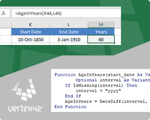
Example #4: Calculate Age for Years Prior to 1900
The Excel function DATEDIF(start_date,end_date,»y») is a very simple way to calculate the age of a person if the dates are after 1/1/1900. The VBA date functions like Year(), Month(), Day(), DateSerial(), DateValue() are able to handle all the Gregorian dates, so custom functions based on the VBA functions can allow you to work with dates prior to 1900. The function below is designed to work like DATEDIF(start_date,end_date,»y») as long as end_date >= start_date.
=AgeInYears(start_date,end_date)
Example: =AgeInYears(«10-Oct-1850″,»5-Jan-1910») returns the value 59.
Function AgeInYears(start_date As Variant, end_date As Variant) As Variant
    AgeInYears = Year(end_date) - Year(start_date) - _
    Abs(DateSerial(Year(end_date), Month(start_date), _
    Day(start_date)) > DateValue(end_date))
End Function
More Custom Excel Function Examples
For an excellent explanation of pretty much everything you need to know to create your own custom Excel function, I would recommend Excel 2016 Formulas. The book provides many good user defined function examples, so if you like to learn by example, it is a great resource.
- Rounding Significant Figures in Excel :: Shows how to return #NUM and #N/A error values.
- UDF Examples — www.ozgrid.com — Provides many examples of user defined functions, including random numbers, hyperlinks, count sum, sort by colors, etc.
- Build an Excel Add-In — http://www.fontstuff.com/vba/vbatut03.htm — An excellent tutorial that takes you through building an add-in for a custom excel function.
Note: I originally published most of this article in 2004, but I’ve updated it significantly and included other examples, as well as the download file.
With VBA, you can create a custom Function (also called a User Defined Function) that can be used in the worksheets just like regular functions.
These are helpful when the existing Excel functions are not enough. In such cases, you can create your own custom User Defined Function (UDF) to cater to your specific needs.
In this tutorial, I’ll cover everything about creating and using custom functions in VBA.
If you’re interested in learning VBA the easy way, check out my Online Excel VBA Training.
What is a Function Procedure in VBA?
A Function procedure is a VBA code that performs calculations and returns a value (or an array of values).
Using a Function procedure, you can create a function that you can use in the worksheet (just like any regular Excel function such as SUM or VLOOKUP).
When you have created a Function procedure using VBA, you can use it in three ways:
- As a formula in the worksheet, where it can take arguments as inputs and returns a value or an array of values.
- As a part of your VBA subroutine code or another Function code.
- In Conditional Formatting.
While there are already 450+ inbuilt Excel functions available in the worksheet, you may need a custom function if:
- The inbuilt functions can’t do what you want to get done. In this case, you can create a custom function based on your requirements.
- The inbuilt functions can get the work done but the formula is long and complicated. In this case, you can create a custom function that is easy to read and use.
Note that custom functions created using VBA can be significantly slower than the inbuilt functions. Hence, these are best suited for situations where you can’t get the result using the inbuilt functions.
Function Vs. Subroutine in VBA
A ‘Subroutine’ allows you to execute a set of code while a ‘Function’ returns a value (or an array of values).
To give you an example, if you have a list of numbers (both positive and negative), and you want to identify the negative numbers, here is what you can do with a function and a subroutine.
A subroutine can loop through each cell in the range and can highlight all the cells that have a negative value in it. In this case, the subroutine ends up changing the properties of the range object (by changing the color of the cells).
With a custom function, you can use it in a separate column and it can return a TRUE if the value in a cell is negative and FALSE if it’s positive. With a function, you can not change the object’s properties. This means that you can not change the color of the cell with a function itself (however, you can do it using conditional formatting with the custom function).
When you create a User Defined Function (UDF) using VBA, you can use that function in the worksheet just like any other function. I will cover more on this in the ‘Different Ways of Using a User Defined Function in Excel’ section.
Creating a Simple User Defined Function in VBA
Let me create a simple user-defined function in VBA and show you how it works.
The below code creates a function that will extract the numeric parts from an alphanumeric string.
Function GetNumeric(CellRef As String) as Long
Dim StringLength As Integer
StringLength = Len(CellRef)
For i = 1 To StringLength
If IsNumeric(Mid(CellRef, i, 1)) Then Result = Result & Mid(CellRef, i, 1)
Next i
GetNumeric = Result
End Function
When you have the above code in the module, you can use this function in the workbook.
Below is how this function – GetNumeric – can be used in Excel.
Now before I tell you how this function is created in VBA and how it works, there are a few things you should know:
- When you create a function in VBA, it becomes available in the entire workbook just like any other regular function.
- When you type the function name followed by the equal to sign, Excel will show you the name of the function in the list of matching functions. In the above example, when I entered =Get, Excel showed me a list that had my custom function.
I believe this is a good example when you can use VBA to create a simple-to-use function in Excel. You can do the same thing with a formula as well (as shown in this tutorial), but that becomes complicated and hard to understand. With this UDF, you only need to pass one argument and you get the result.
Anatomy of a User Defined Function in VBA
In the above section, I gave you the code and showed you how the UDF function works in a worksheet.
Now let’s deep dive and see how this function is created. You need to place the below code in a module in the VB Editor. I cover this topic in the section – ‘Where to put the VBA Code for a User-Defined Function’.
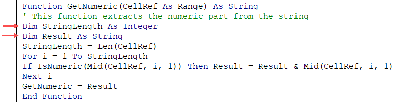
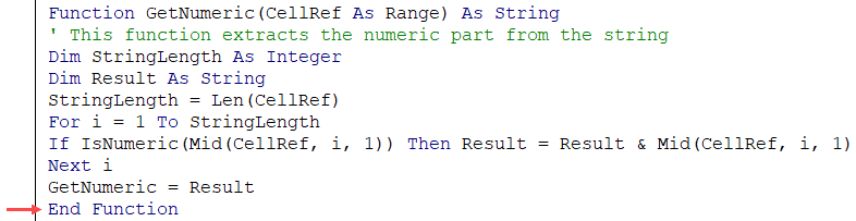
Function GetNumeric(CellRef As String) as Long
' This function extracts the numeric part from the string
Dim StringLength As Integer
StringLength = Len(CellRef)
For i = 1 To StringLength
If IsNumeric(Mid(CellRef, i, 1)) Then Result = Result & Mid(CellRef, i, 1)
Next i
GetNumeric = Result
End Function
The first line of the code starts with the word – Function.
This word tells VBA that our code is a function (and not a subroutine). The word Function is followed by the name of the function – GetNumeric. This is the name that we will be using in the worksheet to use this function.
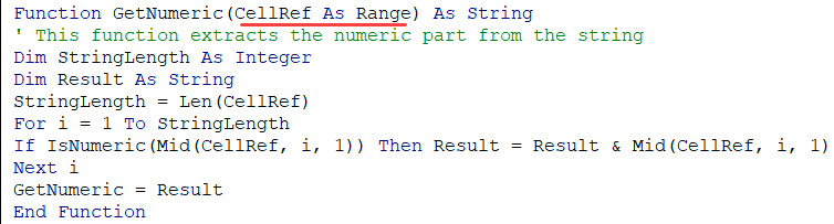
- The name of the function cannot have spaces in it. Also, you can’t name a function if it clashes with the name of a cell reference. For example, you can not name the function ABC123 as it also refers to a cell in Excel worksheet.
- You shouldn’t give your function the same name as that of an existing function. If you do this, Excel would give preference to the in-built function.
- You can use an underscore if you want to separate words. For example, Get_Numeric is an acceptable name.
The function name is followed by some arguments in parenthesis. These are the arguments that our function would need from the user. These are just like the arguments that we need to supply to Excel’s inbuilt functions. For example in a COUNTIF function, there are two arguments (range and criteria)
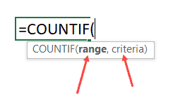
Within the parenthesis, you need to specify the arguments.
In our example, there is only one argument – CellRef.
It’s also a good practice to specify what kind of argument the function expects. In this example, since we will be feeding the function a cell reference, we can specify the argument as a ‘Range’ type. If you don’t specify a data type, VBA would consider it to be a variant (which means you can use any data type).
If you have more than one arguments, you can specify those in the same parenthesis – separated by a comma. We will see later in this tutorial on how to use multiple arguments in a user-defined function.
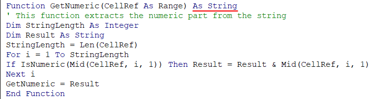
Note that the function is specified as the ‘String’ data type. This would tell VBA that the result of the formula would be of the String data type.
While I can use a numeric data type here (such as Long or Double), doing that would limit the range of numbers it can return. If I have a 20 number long string that I need to extract from the overall string, declaring the function as a Long or Double would give an error (as the number would be out of its range). Hence I have kept the function output data type as String.
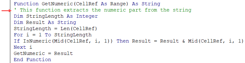
The second line of the code – the one in green that starts with an apostrophe – is a comment. When reading the code, VBA ignores this line. You can use this to add a description or a detail about the code.
The third line of the code declares a variable ‘StringLength’ as an Integer data type. This is the variable where we store the value of the length of the string that is being analyzed by the formula.
The fourth line declares the variable Result as a String data type. This is the variable where we will extract the numbers from the alphanumeric string.
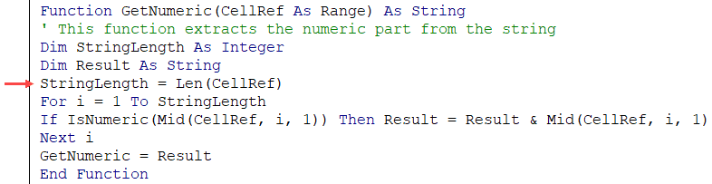
The fifth line assigns the length of the string in the input argument to the ‘StringLength’ variable. Note that ‘CellRef’ refers to the argument that will be given by the user while using the formula in the worksheet (or using it in VBA – which we will see later in this tutorial).
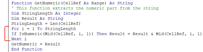
Sixth, seventh, and eighth lines are the part of the For Next loop. The loop runs for as many times as many characters are there in the input argument. This number is given by the LEN function and is assigned to the ‘StringLength’ variable.
So the loop runs from ‘1 to Stringlength’.
Within the loop, the IF statement analyzes each character of the string and if it’s numeric, it adds that numeric character to the Result variable. It uses the MID function in VBA to do this.
The second last line of the code assigns the value of the result to the function. It’s this line of code that ensures that the function returns the ‘Result’ value back in the cell (from where it’s called).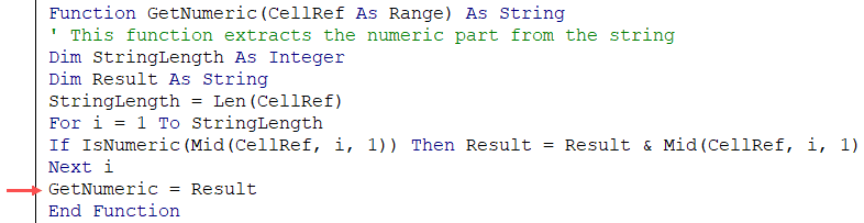
The last line of the code is End Function. This is a mandatory line of code that tells VBA that the function code ends here.
The above code explains the different parts of a typical custom function created in VBA. In the following sections, we will deep dive into these elements and also see the different ways to execute the VBA function in Excel.
Arguments in a User Defined Function in VBA
In the above examples, where we created a user-defined function to get the numeric part from an alphanumeric string (GetNumeric), the function was designed to take one single argument.
In this section, I will cover how to create functions that take no argument to the ones that take multiple arguments (required as well as optional arguments).
Creating a Function in VBA without Any Arguments
In Excel worksheet, we have several functions that take no arguments (such as RAND, TODAY, NOW).
These functions are not dependent on any input arguments. For example, the TODAY function would return the current date and the RAND function would return a random number between 0 and 1.
You can create such similar function in VBA as well.
Below is the code that will give you the name of the file. It doesn’t take any arguments as the result it needs to return is not dependent on any argument.
Function WorkbookName() As String
WorkbookName = ThisWorkbook.Name
End Function
The above code specifies the function’s result as a String data type (as the result we want is the file name – which is a string).
This function assigns the value of ‘ThisWorkbook.Name’ to the function, which is returned when the function is used in the worksheet.
If the file has been saved, it returns the name with the file extension, else it simply gives the name.
The above has one issue though.
If the file name changes, it wouldn’t automatically update. Normally a function refreshes whenever there is a change in the input arguments. But since there are no arguments in this function, the function doesn’t recalculate (even if you change the name of the workbook, close it and then reopen again).
If you want, you can force a recalculation by using the keyboard shortcut – Control + Alt + F9.
To make the formula recalculate whenever there is a change in the worksheet, you need to a line of code to it.
The below code makes the function recalculate whenever there is a change in the worksheet (just like other similar worksheet functions such as TODAY or RAND function).
Function WorkbookName() As String
Application.Volatile True
WorkbookName = ThisWorkbook.Name
End Function
Now, if you change the workbook name, this function would update whenever there is any change in the worksheet or when you reopen this workbook.
Creating a Function in VBA with One Argument
In one of the sections above, we have already seen how to create a function that takes only one argument (the GetNumeric function covered above).
Let’s create another simple function that takes only one argument.
Function created with the below code would convert the referenced text into uppercase. Now we already have a function for it in Excel, and this function is just to show you how it works. If you have to do this, it’s better to use the inbuilt UPPER function.
Function ConvertToUpperCase(CellRef As Range)
ConvertToUpperCase = UCase(CellRef)
End Function
This function uses the UCase function in VBA to change the value of the CellRef variable. It then assigns the value to the function ConvertToUpperCase.
Since this function takes an argument, we don’t need to use the Application.Volatile part here. As soon as the argument changes, the function would automatically update.
Creating a Function in VBA with Multiple Arguments
Just like worksheet functions, you can create functions in VBA that takes multiple arguments.
The below code would create a function that will extract the text before the specified delimiter. It takes two arguments – the cell reference that has the text string, and the delimiter.
Function GetDataBeforeDelimiter(CellRef As Range, Delim As String) as String
Dim Result As String
Dim DelimPosition As Integer
DelimPosition = InStr(1, CellRef, Delim, vbBinaryCompare) - 1
Result = Left(CellRef, DelimPosition)
GetDataBeforeDelimiter = Result
End Function
When you need to use more than one argument in a user-defined function, you can have all the arguments in the parenthesis, separated by a comma.
Note that for each argument, you can specify a data type. In the above example, ‘CellRef’ has been declared as a range datatype and ‘Delim’ has been declared as a String data type. If you don’t specify any data type, VBA considers these are a variant data type.
When you use the above function in the worksheet, you need to give the cell reference that has the text as the first argument and the delimiter character(s) in double quotes as the second argument.
It then checks for the position of the delimiter using the INSTR function in VBA. This position is then used to extract all the characters before the delimiter (using the LEFT function).
Finally, it assigns the result to the function.
This formula is far from perfect. For example, if you enter a delimiter that is not found in the text, it would give an error. Now you can use the IFERROR function in the worksheet to get rid of the errors, or you can use the below code that returns the entire text when it can’t find the delimiter.
Function GetDataBeforeDelimiter(CellRef As Range, Delim As String) as String
Dim Result As String
Dim DelimPosition As Integer
DelimPosition = InStr(1, CellRef, Delim, vbBinaryCompare) - 1
If DelimPosition < 0 Then DelimPosition = Len(CellRef)
Result = Left(CellRef, DelimPosition)
GetDataBeforeDelimiter = Result
End Function
We can further optimize this function.
If you enter the text (from which you want to extract the part before the delimiter) directly in the function, it would give you an error. Go ahead.. try it!
This happens as we have specified the ‘CellRef’ as a range data type.
Or, if you want the delimiter to be in a cell and use the cell reference instead of hard coding it in the formula, you can’t do that with the above code. It’s because the Delim has been declared as a string datatype.
If you want the function to have the flexibility to accept direct text input or cell references from the user, you need to remove the data type declaration. This would end up making the argument as a variant data type, which can take any type of argument and process it.
The below code would do this:
Function GetDataBeforeDelimiter(CellRef, Delim) As String
Dim Result As String
Dim DelimPosition As Integer
DelimPosition = InStr(1, CellRef, Delim, vbBinaryCompare) - 1
If DelimPosition < 0 Then DelimPosition = Len(CellRef)
Result = Left(CellRef, DelimPosition)
GetDataBeforeDelimiter = Result
End Function
Creating a Function in VBA with Optional Arguments
There are many functions in Excel where some of the arguments are optional.
For example, the legendary VLOOKUP function has 3 mandatory arguments and one optional argument.
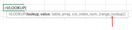
An optional argument, as the name suggests, is optional to specify. If you don’t specify one of the mandatory arguments, your function is going to give you an error, but if you don’t specify the optional argument, your function would work.
But optional arguments are not useless. They allow you to choose from a range of options.
For example, in the VLOOKUP function, if you don’t specify the fourth argument, VLOOKUP does an approximate lookup and if you specify the last argument as FALSE (or 0), then it does an exact match.
Remember that the optional arguments must always come after all the required arguments. You can’t have optional arguments at the beginning.
Now let’s see how to create a function in VBA with optional arguments.
Function with Only an Optional Argument
As far as I know, there is no inbuilt function that takes optional arguments only (I can be wrong here, but I can’t think of any such function).
But we can create one with VBA.
Below is the code of the function that will give you the current date in the dd-mm-yyyy format if you don’t enter any argument (i.e. leave it blank), and in “dd mmmm, yyyy” format if you enter anything as the argument (i.e., anything so that the argument is not blank).
Function CurrDate(Optional fmt As Variant)
Dim Result
If IsMissing(fmt) Then
CurrDate = Format(Date, "dd-mm-yyyy")
Else
CurrDate = Format(Date, "dd mmmm, yyyy")
End If
End Function
Note that the above function uses ‘IsMissing’ to check whether the argument is missing or not. To use the IsMissing function, your optional argument must be of the variant data type.
The above function works no matter what you enter as the argument. In the code, we only check if the optional argument is supplied or not.
You can make this more robust by taking only specific values as arguments and showing an error in rest of the cases (as shown in the below code).
Function CurrDate(Optional fmt As Variant)
Dim Result
If IsMissing(fmt) Then
CurrDate = Format(Date, "dd-mm-yyyy")
ElseIf fmt = 1 Then
CurrDate = Format(Date, "dd mmmm, yyyy")
Else
CurrDate = CVErr(xlErrValue)
End If
End Function
The above code creates a function that shows the date in the “dd-mm-yyyy” format if no argument is supplied, and in “dd mmmm,yyyy” format when the argument is 1. It gives an error in all other cases.
Function with Required as well as Optional Arguments
We have already seen a code that extracts the numeric part from a string.
Now let’s have a look at a similar example that takes both required as well as optional arguments.
The below code creates a function that extracts the text part from a string. If the optional argument is TRUE, it gives the result in uppercase, and if the optional argument is FALSE or is omitted, it gives the result as is.
Function GetText(CellRef As Range, Optional TextCase = False) As String
Dim StringLength As Integer
Dim Result As String
StringLength = Len(CellRef)
For i = 1 To StringLength
If Not (IsNumeric(Mid(CellRef, i, 1))) Then Result = Result & Mid(CellRef, i, 1)
Next i
If TextCase = True Then Result = UCase(Result)
GetText = Result
End Function
Note that in the above code, we have initialized the value of ‘TextCase’ as False (look within the parenthesis in the first line).
By doing this, we have ensured that the optional argument starts with the default value, which is FALSE. If the user specifies the value as TRUE, the function returns the text in upper case, and if the user specifies the optional argument as FALSE or omits it, then the text returned is as is.
Creating a Function in VBA with an Array as the Argument
So far we have seen examples of creating a function with Optional/Required arguments – where these arguments were a single value.
You can also create a function that can take an array as the argument. In Excel worksheet functions, there are many functions that take array arguments, such as SUM, VLOOKUP, SUMIF, COUNTIF, etc.
Below is the code that creates a function that gives the sum of all the even numbers in the specified range of the cells.
Function AddEven(CellRef as Range)
 Dim Cell As Range
 For Each Cell In CellRef
 If IsNumeric(Cell.Value) Then
 If Cell.Value Mod 2 = 0 Then
 Result = Result + Cell.Value
 End If
 End If
 Next Cell
 AddEven = Result
 End Function
You can use this function in the worksheet and provide the range of cells that have the numbers as the argument. The function would return a single value – the sum of all the even numbers (as shown below).
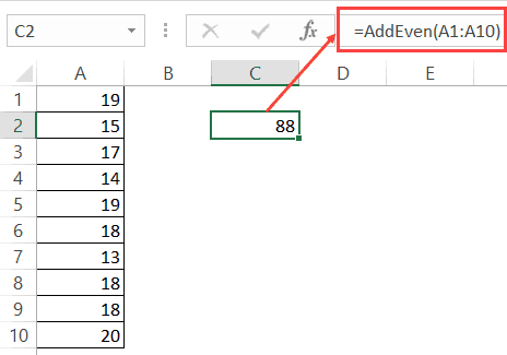
In the above function, instead of a single value, we have supplied an array (A1:A10). For this to work, you need to make sure your data type of the argument can accept an array.
In the code above, I specified the argument CellRef as Range (which can take an array as the input). You can also use the variant data type here.
In the code, there is a For Each loop that goes through each cell and checks if it’s a number of not. If it isn’t, nothing happens and it moves to the next cell. If it’s a number, it checks if it’s even or not (by using the MOD function).
In the end, all the even numbers are added and teh sum is assigned back to the function.
Creating a Function with Indefinite Number of Arguments
While creating some functions in VBA, you may not know the exact number of arguments that a user wants to supply. So the need is to create a function that can accept as many arguments are supplied and use these to return the result.
An example of such worksheet function is the SUM function. You can supply multiple arguments to it (such as this):
=SUM(A1,A2:A4,B1:B20)
The above function would add the values in all these arguments. Also, note that these can be a single cell or an array of cells.
You can create such a function in VBA by having the last argument (or it could be the only argument) as optional. Also, this optional argument should be preceded by the keyword ‘ParamArray’.
‘ParamArray’ is a modifier that allows you to accept as many arguments as you want. Note that using the word ParamArray before an argument makes the argument optional. However, you don’t need to use the word Optional here.
Now let’s create a function that can accept an arbitrary number of arguments and would add all the numbers in the specified arguments:
Function AddArguments(ParamArray arglist() As Variant)
For Each arg In arglist
AddArguments = AddArguments + arg
Next arg
End Function
The above function can take any number of arguments and add these arguments to give the result.
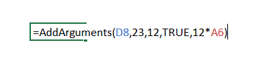
Note that you can only use a single value, a cell reference, a boolean, or an expression as the argument. You can not supply an array as the argument. For example, if one of your arguments is D8:D10, this formula would give you an error.
If you want to be able to use both multi-cell arguments you need to use the below code:
Function AddArguments(ParamArray arglist() As Variant)
For Each arg In arglist
For Each Cell In arg
AddArguments = AddArguments + Cell
Next Cell
Next arg
End Function
Note that this formula works with multiple cells and array references, however, it can not process hardcoded values or expressions. You can create a more robust function by checking and treating these conditions, but that’s not the intent here.
The intent here is to show you how ParamArray works so you can allow an indefinite number of arguments in the function. In case you want a better function than the one created by the above code, use the SUM function in the worksheet.
Creating a Function that Returns an Array
So far we have seen functions that return a single value.
With VBA, you can create a function that returns a variant that can contain an entire array of values.
Array formulas are also available as inbuilt functions in Excel worksheets. If you’re familiar with array formulas in Excel, you would know that these are entered using Control + Shift + Enter (instead of just the Enter). You can read more about array formulas here. If you don’t know about array formulas, don’t worry, keep reading.
Let’s create a formula that returns an array of three numbers (1,2,3).
The below code would do this.
Function ThreeNumbers() As Variant
Dim NumberValue(1 To 3)
NumberValue(1) = 1
NumberValue(2) = 2
NumberValue(3) = 3
ThreeNumbers = NumberValue
End Function
In the above code, we have specified the ‘ThreeNumbers’ function as a variant. This allows it to hold an array of values.
The variable ‘NumberValue’ is declared as an array with 3 elements. It holds the three values and assigns it to the ‘ThreeNumbers’ function.
You can use this function in the worksheet by entering the function and hitting the Control + Shift + Enter key (hold the Control and the Shift keys and then press Enter).
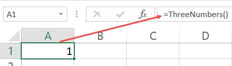
When you do this, it will return 1 in the cell, but in reality, it holds all the three values. To check this, use the below formula:
=MAX(ThreeNumbers())
Use the above function with Control + Shift + Enter. You will notice that the result is now 3, as it is the largest values in the array returned by the Max function, which gets the three numbers as the result of our user-defined function – ThreeNumbers.
You can use the same technique to create a function that returns an array of Month Names as shown by the below code:
Function Months() As Variant
Dim MonthName(1 To 12)
MonthName(1) = "January"
MonthName(2) = "February"
MonthName(3) = "March"
MonthName(4) = "April"
MonthName(5) = "May"
MonthName(6) = "June"
MonthName(7) = "July"
MonthName(8) = "August"
MonthName(9) = "September"
MonthName(10) = "October"
MonthName(11) = "November"
MonthName(12) = "December"
Months = MonthName
End Function
Now when you enter the function =Months() in Excel worksheet and use Control + Shift + Enter, it will return the entire array of month names. Note that you see only January in the cell as that is the first value in the array. This does not mean that the array is only returning one value.
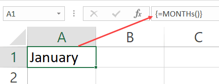
To show you the fact that it is returning all the values, do this – select the cell with the formula, go to the formula bar, select the entire formula and press F9. This will show you all the values that the function returns.

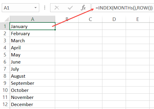
You can use this by using the below INDEX formula to get a list of all the month names in one go.
=INDEX(Months(),ROW())
Now if you have a lot of values, it’s not a good practice to assign these values one by one (as we have done above). Instead, you can use the Array function in VBA.
So the same code where we create the ‘Months’ function would become shorter as shown below:
Function Months() As Variant
Months = Array("January", "February", "March", "April", "May", "June", _
"July", "August", "September", "October", "November", "December")
End Function
The above function uses the Array function to assign the values directly to the function.
Note that all the functions created above return a horizontal array of values. This means that if you select 12 horizontal cells (let’s say A1:L1), and enter the =Months() formula in cell A1, it will give you all the month names.
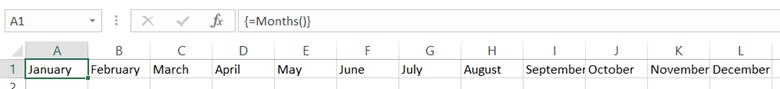
But what if you want these values in a vertical range of cells.
You can do this by using the TRANSPOSE formula in the worksheet.
Simply select 12 vertical cells (contiguous), and enter the below formula.
Understanding the Scope of a User Defined Function in Excel
A function can have two scopes – Public or Private.
- A Public scope means that the function is available for all the sheets in the workbook as well as all the procedures (Sub and Function) across all modules in the workbook. This is useful when you want to call a function from a subroutine (we will see how this is done in the next section).
- A Private scope means that the function is available only in the module in which it exists. You can’t use it in other modules. You also won’t see it in the list of functions in the worksheet. For example, if your Function name is ‘Months()’, and you type function in Excel (after the = sign), it will not show you the function name. You can, however, still, use it if you enter the formula name.
If you don’t specify anything, the function is a Public function by default.
Below is a function that is a Private function:
Private Function WorkbookName() As String
WorkbookName = ThisWorkbook.Name
End Function
You can use this function in the subroutines and the procedures in the same modules, but can’t use it in other modules. This function would also not show up in the worksheet.
The below code would make this function Public. It will also show up in the worksheet.
Function WorkbookName() As String
WorkbookName = ThisWorkbook.Name
End Function
Different Ways of Using a User Defined Function in Excel
Once you have created a user-defined function in VBA, you can use it in many different ways.
Let’s first cover how to use the functions in the worksheet.
Using UDFs in Worksheets
We have already seen examples of using a function created in VBA in the worksheet.
All you need to do is enter the functions name, and it shows up in the intellisense.
Note that for the function to show up in the worksheet, it must be a Public function (as explained in the section above).
You can also use the Insert Function dialog box to insert the user defined function (using the steps below). This would work only for functions that are Public.
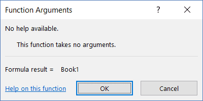
The above steps would insert the function in the worksheet. It also displays a Function Arguments dialog box that will give you details on the arguments and the result.
You can use a user defined function just like any other function in Excel. This also means that you can use it with other inbuilt Excel functions. For example. the below formula would give the name of the workbook in upper case:
=UPPER(WorkbookName())
Using User Defined Functions in VBA Procedures and Functions
When you have created a function, you can use it in other sub-procedures as well.
If the function is Public, it can be used in any procedure in the same or different module. If it’s Private, it can only be used in the same module.
Below is a function that returns the name of the workbook.
Function WorkbookName() As String
WorkbookName = ThisWorkbook.Name
End Function
The below procedure call the function and then display the name in a message box.
Sub ShowWorkbookName()
MsgBox WorkbookName
End Sub
You can also call a function from another function.
In the below codes, the first code returns the name of the workbook, and the second one returns the name in uppercase by calling the first function.
Function WorkbookName() As String
WorkbookName = ThisWorkbook.Name
End Function
Function WorkbookNameinUpper()
WorkbookNameinUpper = UCase(WorkbookName)
End Function
Calling a User Defined Function from Other Workbooks
If you have a function in a workbook, you can call this function in other workbooks as well.
There are multiple ways to do this:
- Creating an Add-in
- Saving function in the Personal Macro Workbook
- Referencing the function from another workbook.
Creating an Add-in
By creating and installing an add-in, you will have the custom function in it available in all the workbooks.
Suppose you have created a custom function – ‘GetNumeric’ and you want it in all the workbooks. To do this, create a new workbook and have the function code in a module in this new workbook.
Now follow the steps below to save it as an add-in and then install it in Excel.
Now the add-in has been activated.
Now you can use the custom function in all the workbooks.
Saving the Function in Personal Macro Workbook
A Personal Macro Workbook is a hidden workbook in your system that opens whenever you open the Excel application.
It’s a place where you can store macro codes and then access these macros from any workbook. It’s a great place to store those macros that you want to use often.
By default, there is no personal macro workbook in your Excel. You need to create it by recording a macro and saving it in the Personal macro workbook.
You can find the detailed steps on how to create and save macros in the personal macro workbook here.
Referencing the function from another workbook
While the first two methods (creating an add-in and using personal macro workbook) would work in all situations, if you want to reference the function from another workbook, that workbook needs to be open.
Suppose you have a workbook with the name ‘Workbook with Formula’, and it has the function with the name ‘GetNumeric’.
To use this function in another workbook (while the Workbook with Formula is open), you can use the below formula:
=’Workbook with Formula’!GetNumeric(A1)
The above formula will use the user defined function in the Workbook with Formula file and give you the result.
Note that since the workbook name has spaces, you need to enclose it in single quotes.
Using Exit Function Statement VBA
If you want to exit a function while the code is running, you can do that by using the ‘Exit Function’ statement.
The below code would extract the first three numeric characters from an alphanumeric text string. As soon as it gets the three characters, the function ends and returns the result.
Function GetNumericFirstThree(CellRef As Range) As Long
Dim StringLength As Integer
StringLength = Len(CellRef)
For i = 1 To StringLength
If J = 3 Then Exit Function
If IsNumeric(Mid(CellRef, i, 1)) Then
J = J + 1
Result = Result & Mid(CellRef, i, 1)
GetNumericFirstThree = Result
End If
Next i
End Function
The above function checks for the number of characters that are numeric, and when it gets 3 numeric characters, it Exits the function in the next loop.
Debugging a User Defined Function
There are a few techniques you can use while debugging a user-defined function in VBA:
Debugging a Custom Function by Using the Message Box
Use MsgBox function to show a message box with a specific value.
The value you display can be based on what you want to test. For example, if you want to check if the code is getting executed or not, any message would work, and if you want to check whether the loops are working or not, you can display a specific value or the loop counter.
Debugging a Custom Function by Setting the Breakpoint
Set a breakpoint to be able to go step through each line one at a time. To set a breakpoint, select the line where you want it and press F9, or click on the gray vertical area which is left to the code lines. Any of these methods would insert a breakpoint (you will see a red dot in the gray area).
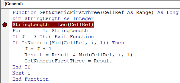
Once you have set the breakpoint and you execute the function, it goes till the breakpoint line and then stops. Now you can step through the code using the F8 key. Pressing F8 once moves to the next line in the code.
Debugging a Custom Function by Using Debug.Print in the Code
You can use Debug.Print statement in your code to get the values of the specified variables/arguments in the immediate window.
For example, in the below code, I have used Debug.Print to get the value of two variables – ‘j’ and ‘Result’
Function GetNumericFirstThree(CellRef As Range) As Long
Dim StringLength As Integer
StringLength = Len(CellRef)
For i = 1 To StringLength
If J = 3 Then Exit Function
If IsNumeric(Mid(CellRef, i, 1)) Then
 J = J + 1
 Result = Result & Mid(CellRef, i, 1)
 Debug.Print J, Result
 GetNumericFirstThree = Result
End If
Next i
End Function
When this code is executed, it shows the following in the immediate window.
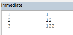
Excel Inbuilt Functions Vs. VBA User Defined Function
There are few strong benefits of using Excel in-built functions over custom functions created in VBA.
- Inbuilt functions are a lot faster than the VBA functions.
- When you create a report/dashboard using VBA functions, and you send it to a client/colleague, they wouldn’t have to worry about whether the macros are enabled or not. In some cases, clients/customers get scared by seeing a warning in the yellow bar (which simply asks them to enable macros).
- With inbuilt Excel functions, you don’t need to worry about file extensions. If you have macros or user-defined functions in the workbook, you need to save it in .xlsm.
While there are many strong reasons to use Excel in-built functions, in a few cases, you’re better off using a user-defined function.
- It’s better to use a user-defined function if your inbuilt formula is huge and complicated. This becomes even more relevant when you need someone else to update the formulas. For example, if you have a huge formula made up of many different functions, even changing a reference to a cell can be tedious and error-prone. Instead, you can create a custom function that only takes one or two arguments and does all the heavy lifting the backend.
- When you have to get something done that can not be done by Excel inbuilt functions. An example of this can be when you want to extract all the numeric characters from a string. In such cases, the benefit of using a user-defined function gar outweighs its negatives.
Where to put the VBA Code for a User-Defined Function
When creating a custom function, you need to put the code in the code window for the workbook in which you want the function.
Below are the steps to put the code for the ‘GetNumeric’ function in the workbook.
- Go to the Developer tab.

- Click on the Visual Basic option. This will open the VB editor in the backend.
- In the Project Explorer pane in the VB Editor, right-click on any object for the workbook in which you want to insert the code. If you don’t see the Project Explorer go to the View tab and click on Project Explorer.
- Go to Insert and click on Module. This will insert a module object for your workbook.

- Copy and paste the code in the module window.

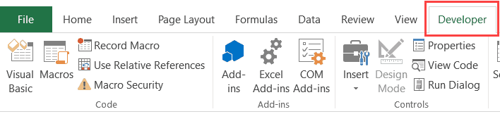
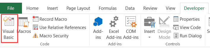
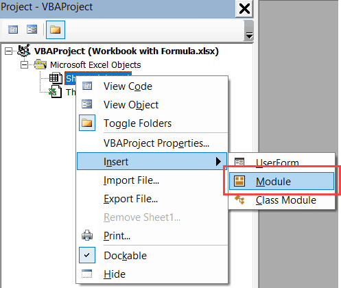
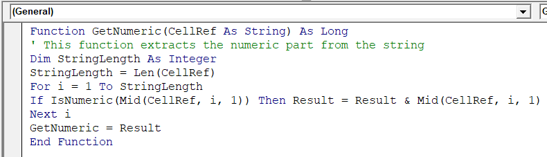
You May Also Like the Following Excel VBA Tutorials:
- Working with Cells and Ranges in Excel VBA.
- Working with Worksheets in Excel VBA.
- Working with Workbooks using VBA.
- How to use Loops in Excel VBA.
- Excel VBA Events – An Easy (and Complete) Guide
- Using IF Then Else Statements in VBA.
- How to Record a Macro in Excel.
- How to Run a Macro in Excel.
- How to Sort Data in Excel using VBA (A Step-by-Step Guide).
- Excel VBA InStr Function – Explained with Examples.
![]()
Download Article
![]()
Download Article
Microsoft Excel has many built-in functions, such as SUM, VLOOKUP, and LEFT. As you start using Excel for more complicated tasks, you may find that you need a function that doesn’t exist. That’s where custom functions come in! This wikiHow teaches you how to create your own functions in Microsoft Excel.
-
1
Open an Excel workbook. Double-click the workbook in which you want to use the custom-defined function to open it in Excel.
-
2
Press Alt+F11 (Windows) or Fn+⌥ Opt+F11 (Mac). This opens the Visual Basic Editor.
Advertisement
-
3
Click the Insert menu and select New Module. This opens a module window in the right panel of the editor.[1]
- You can create the user defined function in the worksheet itself without adding a new module, but that will make you unable to use the function in other worksheets of the same workbook.
-
4
Create your function’s header. The first line is where you will name the function and define our range.[2]
Replace «FunctionName» with the name you want to assign your custom function. The function can have as many parameters as you want, and their types can be any of Excel’s basic data or object types as Range:Function FunctionName (param1 As type1, param2 As type2 ) As return Type
- You may think of parameters as the «operands» your function will act upon. For example, when you use SIN(45) to calculate the Sine of 45 degree, 45 will be taken as a parameter. Then the code of your function will use that value to calculate something else and present the result.
-
5
Add the code of the function. Make sure you use the values provided by the parameters, assign the result to the name of the function, and close the function with «End Function.» Learning to program in VBA or in any other language can take some time and a detailed tutorial. However, functions usually have small code blocks and use very few features of the language. Some useful elements are:
- The If block, which allows you to execute a part of the code only if a condition is met. Notice the elements in an If code block: IF condition THEN code ELSE code END IF. The Else keyword along with the second part of the code are optional:
Function Course Result(grade As Integer) As String
  If grade >= 5 Then
    CourseResult = "Approved"
  Else
    CourseResult = "Rejected"
  End If
End Function
- The Do block, which executes a part of the code While or Until a condition is met. In the example code below, notice the elements DO code LOOP WHILE/UNTIL condition. Also notice the second line in which a variable is declared. You can add variables to your code so you can use them later. Variables act as temporary values inside the code. Finally, notice the declaration of the function as BOOLEAN, which is a datatype that allows only the TRUE and FALSE values. This method of determining if a number is prime is by far not the optimal, but I’ve left it that way to make the code easier to read.
Function IsPrime(value As Integer) As Boolean
  Dim i As Integer
  i = 2
  IsPrime = True
  Do
    If value / i = Int(value / i) Then
      IsPrime = False
    End If
    i = i + 1
  Loop While i < value And IsPrime = True
End Function
- The For block executes a part of the code a specified number of times. In this next example, you’ll see the elements FOR variable = lower limit TO upper limit code NEXT. You’ll also see the added ElseIf element in the If statement, which allows you to add more options to the code that is to be executed. Additionally, the declaration of the function and the variable result as Long. The Long datatype allows values much larger than Integer:
Public Function Factorial(value As Integer) As Long
  Dim result As Long
  Dim i As Integer
  If value = 0 Then
    result = 1
  ElseIf value = 1 Then
    result = 1
  Else
    result = 1
    For i = 1 To value
      result = result * i
    Next
  End If
  Factorial = result
End Function
- The If block, which allows you to execute a part of the code only if a condition is met. Notice the elements in an If code block: IF condition THEN code ELSE code END IF. The Else keyword along with the second part of the code are optional:
-
6
Close the Visual Basic Editor. Once you’ve created your function, close the window to return to your workbook. Now you can start using your user-defined function.
-
7
Enter your function. First, click the cell in which you want to enter the function. Then, click the function bar at the top of Excel (the one with the fx to its left) and type =FUNCTIONNAME(), replacing FUNCTIONNAME with the name you assigned your custom function.
- You can also find your user-defined formula in the «User Defined» category in the Insert Formula wizard—just click the fx to pull up the wizard.
-
8
Enter the parameters into the parentheses. For example, =NumberToLetters(A4). The parameters can be of three types:
- Constant values typed directly in the cell formula. Strings have to be quoted in this case.
- Cell references like B6 or range references like A1:C3. The parameter has to be of the Range datatype.
- Other functions nested inside your function. Your function can also be nested inside other functions. Example: =Factorial(MAX(D6:D8)).
-
9
Press ↵ Enter or ⏎ Return to run the function. The results will display in the selected cell.


Advertisement
Add New Question
-
Question
How can I use these functions in all Excel files?

Igal Livne
Community Answer
Save the workbook with the custom class as «Excel Add-In (*.xlam»),» by default Excel will take you to «Addins» folder. Go to Excel Options > Add-ins > Manage: «Excel Addins» — press «Go…» button. Browse for your newly create xlam file.
-
Question
How can I do well in exams?
Read the directions several times, leaving time for you to absorb between readings. Also practice writing VBA to do various things.
-
Question
How do I know what to write as the function code?
In order to create functions, you need a skill called «programming». Excel macros are written in a language called «Visual Basic for Applications», which you will need to learn to be able to write macros. It’s quite easy once you’ve got the hang of it though!
Ask a Question
200 characters left
Include your email address to get a message when this question is answered.
Submit
Advertisement
Video
-
Use a name that’s not already defined as a function name in Excel or you’ll end up being able to use only one of the functions.
-
Whenever you write a block of code inside a control structure like If, For, Do, etc. make sure you indent the block of code using a few blank spaces or the Tab key. That will make your code easier to understand and you’ll find a lot easier to spot errors and make improvements.
Show More Tips
Thanks for submitting a tip for review!
Advertisement
-
The functions used in this article are, by no means, the best way to solve the related problems. They were used here only to explain the usage of the control structures of the language.
-
VBA, as any other language, has several other control structures besides Do, If and For. Those have been explained here only to clarify what kind of things can be done inside the function source code. There are many online tutorials available where you can learn VBA.
-
Due to security measures, some people may disable macros. Make sure you let your colleagues know the book you’re sending them has macros and that they can trust they’re not going to damage their computers.
Advertisement
About This Article
Article SummaryX
1. Open Excel.
2. Press Alt + F11 to open the Visual Basic editor.
3. Create the function’s name and set the parameter types.
4. Use VB code to write your function.
5. Close the editor.
6. Run your function as you would other functions.
Did this summary help you?
Thanks to all authors for creating a page that has been read 640,189 times.