Use value in excel

Excel for Microsoft 365 Excel for Microsoft 365 for Mac Excel for the web Excel 2021 Excel 2021 for Mac Excel 2019 Excel 2019 for Mac Excel 2016 Excel 2016 for Mac Excel 2013 Excel 2010 Excel 2007 Excel for Mac 2011 Excel Starter 2010 More…Less

This article describes the formula syntax and usage of the VALUE
 function in Microsoft Excel.

Description

Converts a text string that represents a number to a number.

Syntax

VALUE(text)

The VALUE function syntax has the following arguments:

  • Text    Required. The text enclosed in quotation marks or a reference to a cell containing the text you want to convert.

Remarks

  • Text can be in any of the constant number, date, or time formats recognized by Microsoft Excel. If text is not in one of these formats, VALUE returns the #VALUE! error value.

  • You do not generally need to use the VALUE function in a formula because Excel automatically converts text to numbers as necessary. This function is provided for compatibility with other spreadsheet programs.

Example

Copy the example data in the following table, and paste it in cell A1 of a new Excel worksheet. For formulas to show results, select them, press F2, and then press Enter. If you need to, you can adjust the column widths to see all the data.

Formula

Description

Result

=VALUE(«$1,000»)

Number equivalent of the text string «$1,000»

1000

=VALUE(«16:48:00»)-VALUE(«12:00:00»)

The serial number equivalent to 4 hours and 48 minutes, which is «16:48:00» minus «12:00:00» (0.2 = 4:48).

0.2

Need more help?

Want more options?

Explore subscription benefits, browse training courses, learn how to secure your device, and more.

Communities help you ask and answer questions, give feedback, and hear from experts with rich knowledge.

The VALUE function is a text function that converts a number from text format to numerical format where data is in an Excel-recognized format such as date, currency, time, etc. Mostly, if Excel recognizes a number, it automatically converts the data into numerical format. However, in other cases, we can do so using the VALUE function.

The VALUE function is most helpful when we seek compatibility with other spreadsheet programs and for using the numerical text resulting from text functions in calculations.

Excel VALUE Function

Syntax

The syntax of the VALUE function is quite straightforward and is given below.

=VALUE(text)

Arguments:

The VALUE function accepts only one argument, and it is mandatory.

text‘– This mandatory argument contains the value in text format that needs to be converted. The value of the text argument can be passed as a direct value in double quotes or as a cell reference.

Important Characteristics of the VALUE Function

Some noteworthy features of the VALUE function are as follows.

  • The VALUE function only accepts the value that is recognized by Microsoft Excel such as constant number, locale formatted number, date, or time. If the value of the text argument is any value that is not recognized by Excel, the function results in a #VALUE! error.
  • If the value of the text argument is empty, the VALUE function returns zero.

When using the VALUE function, it is important to note the alignment of the data as left-aligned data indicates text format whereas right-aligned data is number format.

Examples of VALUE Function

There are instances when the given data which looks like a number cannot be used further for calculations and analysis. In such scenarios, the VALUE function comes in very handy. Below are some examples to provide a better understanding of the function.

Example 1 – Simple Use of VALUE Function

In this example, we will use different types of input values for the text argument to better understand the functionality of the VALUE function.

We have taken time, date, date and time together, number in text format, and percentage as the input values. The function used is as follows.

=VALUE(B3)

Simple Use of VALUE Function

In the first example, the value of the text argument is a time value which upon conversion to numerical format is transformed into the serial number. Excel stores time as fractions of a day. The VALUE function simply converted the time format to an actual serial number which can further be used in formulas.

The next example is in date format and like the time data, the VALUE function converts the date value to a sequential number as stored in Excel. The third example is a combination of date and time, and the VALUE function returns the expected result of the corresponding serial number and fraction of both date and time in cell C5.

The fourth example is a text which looks like a number. If we wish to use the data in cell B6 for any calculations, the result will also take on the text format. With the help of the VALUE function, the number is transformed from text format to numerical format.

The last example is a percentage value. The VALUE function returns the calculated numerical value of the percentage which is 0.25 in this case.

Now that the basic functionality of the VALUE function is clear, check some useful applications of the same in the examples below.

Example 2 – Converting String to Number using VALUE Function

In this scenario, we collected small donations from our neighbors to get essentials for the homeless shelter. The data collected was user-generated hence it is in text format.

Converting String to Number using VALUE Function

To calculate the total donations received, we can extract the dollar amount and then sum it up. To segregate the donation amount from the given text, we will use the TEXTBEFORE function. It will extract the characters that occur before the dollar sign ($), which is the amount in this case. The formula used is as follows.

=TEXTBEFORE(B3,"$")

Now that the donation amount is segregated in column C, the total donation can be calculated.

Converting String to Number using VALUE Function

Unfortunately, all the extracted data in column C is text, which is clear due to its left alignment, since the TEXTBEFORE function is a text function. Therefore, the total sum couldn’t be downloaded as seen in cell C10. To rectify this, we will use the VALUE function to convert all the data in column C into the numeric format and then calculate the total donation received. The updated formula to be used is as follows.

=VALUE(TEXTBEFORE(B3,"$"))

Converting String to Number using VALUE Function

We can combine everything in one formula as follows.

=SUM(VALUE(TEXTBEFORE(B3:B8,"$")))

Converting String to Number using VALUE Function

Note: One can also use the LEFT function in place of the TEXTBEFORE function to achieve the same result.

Example 3 – Converting Currency to Numerical Format

Here, in this case, we have received the monthly sales for the last year. As the sales report is from the India office, the currency formatting is different where a comma is used as a group separator in hundreds, thousands, and so on. Excel does not recognize the formatting, so it treats the sales numbers as text.

Converting Currency to Numerical Format

To be able to use the data for further calculations, we wish to convert them from text format to number format. As it is not an Excel-recognized format, the VALUE function will return a #VALUE! error.

Converting Currency to Numerical Format

To overcome this, we can first use the SUBSTITUTE function to replace all the commas with an empty string and then use the VALUE function. The formula used will be as follows.

=SUBSTITUTE(C3,",","")

Converting Currency to Numerical Format

Now the sales values in column D are in a recognizable format i.e. text, with the help of the VALUE function, we can convert the same in number format. Combining both steps, the final formula used will be as follows.

=VALUE(SUBSTITUTE(C3,",",""))

Converting Currency to Numerical Format

As evident by the right alignment of the data in column D, all the sales values are now in a number format and therefore can be further used for calculations.

Example 4 – Converting Time using the VALUE Function

In this example, we are conducting an online test where the completion time is set to 10:00 AM. However, every applicant can take extra time up to 20 minutes, but points will be assigned depending on the extra time taken which will eventually be deducted from the actual score. Here are the points to be deducted as per the completion time.

<p>The VALUE function is a text function that converts a number from text format to numerical format where data is in an Excel-recognized format such as date, currency, time, etc. Mostly, if Excel recognizes a number, it automatically converts the data into numerical format. However, in other cases, we can do so using the VALUE function.</p> <p>The VALUE function is most helpful when we seek compatibility with other spreadsheet programs and for using the numerical text resulting from text functions in calculations.</p> <p><img class="aligncenter size-full wp-image-8529" src="https://exceltrick.com/wp-content/uploads/2023/02/Excel-VALUE-Function.png" alt="Excel VALUE Function" width="753" height="396" /></p> <h2>Syntax</h2> <p>The syntax of the VALUE function is quite straightforward and is given below.</p> <div class="excelFormula"><code><span class="operator">=</span><span class="function">VALUE</span>(text)</code></div> <p style="margin: 0px;"><strong>Arguments:</strong></p> <p>The VALUE function accepts only one argument, and it is mandatory.</p> <p style="padding-left: 30px;">'<em>text</em>'– This mandatory argument contains the value in text format that needs to be converted. The value of the <em>text </em>argument can be passed as a direct value in double quotes or as a cell reference.</p> <h2>Important Characteristics of the VALUE Function</h2> <p>Some noteworthy features of the VALUE function are as follows.</p> <ul> <li>The VALUE function only accepts the value that is recognized by Microsoft Excel such as constant number, locale formatted number, date, or time. If the value of the <em>text </em>argument is any value that is not recognized by Excel, the function results in a #VALUE! error.</li> <li>If the value of the <em>text </em>argument is empty, the VALUE function returns zero.</li> </ul> <p><span style="font-size: revert; color: initial;">When using the VALUE function, it is important to note the alignment of the data as left-aligned data indicates text format whereas right-aligned data is number format.</span></p> <h2>Examples of VALUE Function</h2> <p>There are instances when the given data which looks like a number cannot be used further for calculations and analysis. In such scenarios, the VALUE function comes in very handy. Below are some examples to provide a better understanding of the function.</p> <h3>Example 1 - Simple Use of VALUE Function</h3> <p>In this example, we will use different types of input values for the <em>text </em>argument to better understand the functionality of the VALUE function.</p> <p>We have taken time, date, date and time together, number in text format, and percentage as the input values. The function used is as follows.</p> <div class="excelFormula"><code><span class="operator">=</span><span class="function">VALUE</span>(B3)</code></div> <p><img class="aligncenter size-full wp-image-8530" src="https://exceltrick.com/wp-content/uploads/2023/02/value-function-in-excel_02.png" alt="Simple Use of VALUE Function" width="428" height="256" /></p> <p>In the first example, the value of the <em>text</em> argument is a time value which upon conversion to numerical format is transformed into the serial number. Excel stores time as fractions of a day. The VALUE function simply converted the time format to an actual serial number which can further be used in formulas.</p> <p>The next example is in date format and like the time data, the VALUE function converts the date value to a sequential number as stored in Excel. The third example is a combination of date and time, and the VALUE function returns the expected result of the corresponding serial number and fraction of both date and time in cell C5.</p> <p>The fourth example is a text which looks like a number. If we wish to use the data in cell B6 for any calculations, the result will also take on the text format. With the help of the VALUE function, the number is transformed from text format to numerical format.</p> <p>The last example is a percentage value. The VALUE function returns the calculated numerical value of the percentage which is 0.25 in this case.</p> <p>Now that the basic functionality of the VALUE function is clear, check some useful applications of the same in the examples below.</p> <h3>Example 2 - Converting String to Number using VALUE Function</h3> <p>In this scenario, we collected small donations from our neighbors to get essentials for the homeless shelter. The data collected was user-generated hence it is in text format.</p> <p><img class="aligncenter size-full wp-image-8531" src="https://exceltrick.com/wp-content/uploads/2023/02/value-function-in-excel_03.png" alt="Converting String to Number using VALUE Function" width="429" height="244" /></p> <p>To calculate the total donations received, we can extract the dollar amount and then sum it up. To segregate the donation amount from the given text, we will use the TEXTBEFORE function. It will extract the characters that occur before the dollar sign ($), which is the amount in this case. The formula used is as follows.</p> <div class="excelFormula"><code><span class="operator">=</span><span class="function">TEXTBEFORE</span>(B3,"<span class="string">$</span>")</code></div> <p>Now that the donation amount is segregated in column C, the total donation can be calculated.</p> <p><img class="aligncenter size-full wp-image-8532" src="https://exceltrick.com/wp-content/uploads/2023/02/value-function-in-excel_04.png" alt="Converting String to Number using VALUE Function" width="565" height="305" /></p> <p>Unfortunately, all the extracted data in column C is text, which is clear due to its left alignment, since the TEXTBEFORE function is a text function. Therefore, the total sum couldn't be downloaded as seen in cell C10. To rectify this, we will use the VALUE function to convert all the data in column C into the numeric format and then calculate the total donation received. The updated formula to be used is as follows.</p> <div class="excelFormula"><code><span class="operator">=</span><span class="function">VALUE</span>(<span class="function">TEXTBEFORE</span>(B3,"<span class="string">$</span>"))</code></div> <p><img class="aligncenter size-full wp-image-8533" src="https://exceltrick.com/wp-content/uploads/2023/02/value-function-in-excel_05.png" alt="Converting String to Number using VALUE Function" width="561" height="306" /></p> <p>We can combine everything in one formula as follows.</p> <div class="excelFormula"><code><span class="operator">=</span><span class="function">SUM</span>(<span class="function">VALUE</span>(<span class="function">TEXTBEFORE</span>(B3:B8,"<span class="string">$</span>")))</code></div> <p><img class="aligncenter size-full wp-image-8534" src="https://exceltrick.com/wp-content/uploads/2023/02/value-function-in-excel_06.png" alt="Converting String to Number using VALUE Function" width="545" height="307" /></p> <p><strong>Note:</strong> One can also use the <a href="mailto:https://exceltrick.com/formulas_macros/excel-left-function/">LEFT function</a> in place of the TEXTBEFORE function to achieve the same result.</p> <h3>Example 3 - Converting Currency to Numerical Format</h3> <p>Here, in this case, we have received the monthly sales for the last year. As the sales report is from the India office, the currency formatting is different where a comma is used as a group separator in hundreds, thousands, and so on. Excel does not recognize the formatting, so it treats the sales numbers as text.</p> <p><img class="aligncenter size-full wp-image-8535" src="https://exceltrick.com/wp-content/uploads/2023/02/value-function-in-excel_07.png" alt="Converting Currency to Numerical Format" width="418" height="387" /></p> <p>To be able to use the data for further calculations, we wish to convert them from text format to number format. As it is not an Excel-recognized format, the VALUE function will return a #VALUE! error.</p> <p><img class="aligncenter size-full wp-image-8536" src="https://exceltrick.com/wp-content/uploads/2023/02/value-function-in-excel_08.png" alt="Converting Currency to Numerical Format" width="584" height="426" /></p> <p>To overcome this, we can first use the <a href="mailto:https://exceltrick.com/formulas_macros/excel-substitute-function/">SUBSTITUTE function</a> to replace all the commas with an empty string and then use the VALUE function. The formula used will be as follows.</p> <div class="excelFormula"><code><span class="operator">=</span><span class="function">SUBSTITUTE</span>(C3,"<span class="string">,</span>","")</code></div> <p><img class="aligncenter size-full wp-image-8537" src="https://exceltrick.com/wp-content/uploads/2023/02/value-function-in-excel_09.png" alt="Converting Currency to Numerical Format" width="582" height="426" /></p> <p>Now the sales values in column D are in a recognizable format i.e. text, with the help of the VALUE function, we can convert the same in number format. Combining both steps, the final formula used will be as follows.</p> <div class="excelFormula"><code><span class="operator">=</span><span class="function">VALUE</span>(<span class="function">SUBSTITUTE</span>(C3,"<span class="string">,</span>",""))</code></div> <p><img class="aligncenter size-full wp-image-8538" src="https://exceltrick.com/wp-content/uploads/2023/02/value-function-in-excel_10.png" alt="Converting Currency to Numerical Format" width="585" height="426" /></p> <p>As evident by the right alignment of the data in column D, all the sales values are now in a number format and therefore can be further used for calculations.</p> <h3>Example 4 - Converting Time using the VALUE Function</h3> <p>In this example, we are conducting an online test where the completion time is set to 10:00 AM. However, every applicant can take extra time up to 20 minutes, but points will be assigned depending on the extra time taken which will eventually be deducted from the actual score. Here are the points to be deducted as per the completion time.</p> <p><img 11></p> <p>As the first step, we will calculate the extra time taken in each case. The formula used will be as follows.</p> <div class="excelFormula"><code><span class="operator">=</span>B4<span class="operator">-</span>$C$2</code></div> <p><img 12></p> <p>Now that we have all the values in column C, we can use the <a href=":https://exceltrick.com/formulas_macros/excel-nested-if/">nested IF function</a> to compare the time as per the point system and then assign the corresponding points. However, while using the delayed time data from C4:C7, we will wrap it in the VALUE function to ensure that Excel treats the time value as a number and not text.</p> <p>The logic used will be as follows.</p> <p>If the delayed time (C4) is less than 5 minutes, then assign 1 point, else if the delayed time is less than 10 minutes, assign 2 points….) and so on till 20 minutes. If no condition is met, the formula returns FALSE.</p> <p>The formula used will be as follows.</p> <div class="excelFormula"><code><span class="operator">=</span><span class="function">IF</span>(C4<span class="operator"><</span><span class="function">VALUE</span>("<span class="string">0:05</span>"),1,<span class="function">IF</span>(C4<span class="operator"><</span><span class="function">VALUE</span>("<span class="string">0:10</span>"),2,<span class="function">IF</span>(C4<span class="operator"><</span><span class="function">VALUE</span>("<span class="string">0:15</span>"),3,<span class="function">IF</span>(C4<span class="operator"><</span><span class="function">VALUE</span>("<span class="string">0:20</span>"),4))))</code></div> <p><img 13></p> <p>Now we have the final points that will be deducted from the final score in each case. With the help of the VALUE function, we were able to convert the time value from minutes to numerical format and execute the nested IF function.</p> <h2>VALUE Function vs NUMBERVALUE Function</h2> <p>Both the VALUE and NUMBERVALUE functions convert text that looks like a number from text format to numerical format but the <a href="mailto:https://exceltrick.com/formulas_macros/excel-numbervalue-function/">NUMBERVALUE function</a> transforms the data using the given group and decimal separators which help the function understand the format.</p> <p>If the data is not in an Excel-recognized format, the VALUE function returns a #VALUE! error whereas with the NUMBERVALUE function, we can mention the group and decimal separator used in the data to convert it. Let's understand it better using an example.</p> <p><img 14></p> <p>The data in cell B4 is a currency value in euros and is in a text format. The VALUE function does not recognize the data and hence throws a #VALUE! error whereas the NUMBERVALUE function converts the data from text to number format due to the mentioned decimal and group separator.</p> <h2>VALUE Function vs VALUETOTEXT Function</h2> <p>Now we know that the VALUE function converts text that looks like a number from the text format to numerical format. The VALUETOTEXT function performs the opposite conversion. The VALUETOTEXT function converts a value to text format depending on the concise or strict format.</p> <p>Hopefully, now you have a clear idea about how to use the VALUE function to your advantage. Practice and discover new applications of the said function.</p>

As the first step, we will calculate the extra time taken in each case. The formula used will be as follows.

=B4-$C$2

Converting Time using the VALUE Function

Now that we have all the values in column C, we can use the nested IF function to compare the time as per the point system and then assign the corresponding points. However, while using the delayed time data from C4:C7, we will wrap it in the VALUE function to ensure that Excel treats the time value as a number and not text.

The logic used will be as follows.

If the delayed time (C4) is less than 5 minutes, then assign 1 point, else if the delayed time is less than 10 minutes, assign 2 points….) and so on till 20 minutes. If no condition is met, the formula returns FALSE.

The formula used will be as follows.

=IF(C4<VALUE("0:05"),1,IF(C4<VALUE("0:10"),2,IF(C4<VALUE("0:15"),3,IF(C4<VALUE("0:20"),4))))

Converting Time using the VALUE Function

Now we have the final points that will be deducted from the final score in each case. With the help of the VALUE function, we were able to convert the time value from minutes to numerical format and execute the nested IF function.

VALUE Function vs NUMBERVALUE Function

Both the VALUE and NUMBERVALUE functions convert text that looks like a number from text format to numerical format but the NUMBERVALUE function transforms the data using the given group and decimal separators which help the function understand the format.

If the data is not in an Excel-recognized format, the VALUE function returns a #VALUE! error whereas with the NUMBERVALUE function, we can mention the group and decimal separator used in the data to convert it. Let’s understand it better using an example.

VALUE Function vs NUMBERVALUE Function

The data in cell B4 is a currency value in euros and is in a text format. The VALUE function does not recognize the data and hence throws a #VALUE! error whereas the NUMBERVALUE function converts the data from text to number format due to the mentioned decimal and group separator.

VALUE Function vs VALUETOTEXT Function

Now we know that the VALUE function converts text that looks like a number from the text format to numerical format. The VALUETOTEXT function performs the opposite conversion. The VALUETOTEXT function converts a value to text format depending on the concise or strict format.

Hopefully, now you have a clear idea about how to use the VALUE function to your advantage. Practice and discover new applications of the said function.

Date yes Add (Subtract) Days to a Date Concatenate Dates Convert Date to Number Convert Date to Text Month Name to Number Create Date Range from Dates Day Number of Year Month Name from Date First Day of Month Add (Subtract) Weeks to a Date If Functions with Dates Max Date Number of Days Between Dates Number of Days in a Month Number of Weeks Between Dates Number of Years Between Dates Split Date & Time into Separate Cells Countdown Remaining Days Insert Dates Random Date Generator Using Dynamic Ranges — Year to Date Values Add (Subtract) Years to a Date Date Formula Examples Extract Day from Date Get Day Name from Date Count Days Left in Month / Year Count Workdays Left in Month / Year Get Last Day of Month Last Business Day of Month / Year Number of Work / Business Days in Month Weekday Abbreviations Auto Populate Dates Number of Months Between Dates Quarter from a Date Years of Service Change Date Format Compare Dates Time yes Add (Subtract) Hours to Time Add (Subtract) Minutes to Time Add (Subtract) Seconds to Time Add Up time (Total Time) Time Differences Change Time Format Convert Minutes to Hours Convert Time to Decimal Convert Time to Hours Convert Time to Minutes Convert Time to Seconds Military Time Round Time to Nearest 15 Minutes Overtime Calculator Number of Hours Between Times Convert Seconds to Minutes, Hours, or Time Count Hours Worked Time Differences Time Format — Show Minutes Seconds Text yes Add Commas to Cells Get First Word from Text Capitalize First Letter Clean & Format Phone #s Remove Extra Trailing / Leading Spaces Add Spaces to Cell Assign Number Value to Text Combine Cells with Comma Combine First and Last Names Convert Text String to Date Convert Text to Number Extract Text From Cell Get Last Word Remove Unwated Characters Extract Text Before or After Character How to Split Text String by Space, Comma, & More Remove Special Characters Remove First Characters from Left Substitute Multiple Values Switch First & Last Names w/ Commas Remove Specific Text from a Cell Extract Text Between Characters (Ex. Parenthesis) Add Leading Zeros to a Number Remove Line Breaks from Text Remove all Numbers from Text Reverse Text Remove Non-Numeric Characters Remove Last Character(s) From Right Separate First and Last Names Separate Text & Numbers Round yes Round Formulas Round Price to Nearest Dollar or Cent Round to Nearest 10, 100, or 1000 Round to Nearest 5 or .5 Round Percentages Round to Significant Figures Count yes Count Blank and Non-blank Cells Count Cells Between Two Numbers Count Cells not Equal to Count if Cells are in Range Count Times Word Appears in Cell Count Words in Cell Count Specific Characters in Column Count Total Number of Characters in Column Count Cells that Equal one of two Results Count Cells that do not Contain Count Cells that Contain Specific Text Count Unique Values in Range Countif — Multiple Criteria Count Total Number of Cells in Range Count Cells with Any Text Count Total Cells in a Table Lookup yes Two Dimensional VLOOKUP VLOOKUP Simple Example Vlookup — Multiple Matches Case Sensitive Lookup Case Sensitive VLOOKUP Sum if — VLOOKUP Case Sensitive Lookup Case Sensitive VLOOKUP Find Duplicates w/ VLOOKUP or MATCH INDEX MATCH MATCH Lookup — Return Cell Address (Not Value) Lookup Last Value in Column or Row Reverse VLOOKUP (Right to Left) Risk Score Bucket with VLOOKUP Sum with a VLOOKUP Function VLOOKUP & INDIRECT VLOOKUP Concatenate VLOOKUP Contains (Partial Match) 17 Reasons Why Your XLOOKUP is Not Working Double (Nested) XLOOKUP — Dynamic Columns IFERROR (& IFNA) XLOOKUP Lookup Min / Max Value Nested VLOOKUP Top 11 Alternatives to VLOOKUP (Updated 2022!) VLOOKUP – Dynamic Column Reference VLOOKUP – Fix #N/A Error VLOOKUP – Multiple Sheets at Once VLOOKUP & HLOOKUP Combined VLOOKUP & MATCH Combined VLOOKUP Between Worksheets or Spreadsheets VLOOKUP Duplicate Values VLOOKUP Letter Grades VLOOKUP Return Multiple Columns VLOOKUP Returns 0? Return Blank Instead VLOOKUP w/o #N/A Error XLOOKUP Multiple Sheets at Once XLOOKUP Between Worksheets or Spreadsheets XLOOKUP by Date XLOOKUP Duplicate Values XLOOKUP Multiple Criteria XLOOKUP Return Multiple Columns XLOOKUP Returns 0? Return Blank Instead XLOOKUP Text XLOOKUP with IF XLOOKUP With If Statement Misc. yes Sort Multiple Columns Use Cell Value in Formula Percentage Change Between Numbers Percentage Breakdown Rank Values Add Spaces to Cell CAGR Formula Average Time Decimal Part of Number Integer Part of a Number Compare Items in a List Dealing with NA() Errors Get Worksheet Name Wildcard Characters Hyperlink to Current Folder Compound Interest Formula Percentage Increase Create Random Groups Sort with the Small and Large Functions Non-volatile Function Alternatives Decrease a Number by a Percentage Calculate Percent Variance Profit Margin Calculator Convert Column Number to Letter Get Full Address of Named Range Insert File Name Insert Path Latitute / Longitude Functions Replace Negative Values Reverse List Range Convert State Name to Abbreviation Create Dynamic Hyperlinks Custom Sort List with Formula Data Validation — Custom Formulas Dynamic Sheet Reference (INDIRECT) Reference Cell in Another Sheet or Workbook Get Cell Value by Address Get Worksheet Name Increment Cell Reference List Sheet Names List Skipped Numbers in Sequence Return Address of Max Value in Range Search by Keywords Select Every Other (or Every nth) Row Basics yes Cell Reference Basics — A1, R1C1, 3d, etc. Add Up (Sum) Entire Column or Row Into to Dynamic Array Formulas Conversions yes Convert Time Zones Convert Celsius to Fahrenheit Convert Pounds to Kilograms Convert Time to Unix Time Convert Feet to Meters Convert Centimeters to Inches Convert Kilometers to Miles Convert Inches to Feet Convert Date to Julian Format Convert Column Letter to Number Tests yes Test if a Range Contains any Text Test if any Cell in Range is Number Test if a Cell Contains a Specific Value Test if Cell Contains Any Number Test if Cell Contains Specific Number Test if Cell is Number or Text If yes Percentile If Subtotal If Sumproduct If Large If and Small If Median If Concatentate If Max If Rank If TEXTJOIN If Sum yes Sum if — Begins With / Ends With Sum if — Month or Year to Date Sum if — By Year Sum if — Blank / Non-Blank Sum if — Horizontal Sum Count / Sum If — Cell Color INDIRECT Sum Sum If — Across Multiple Sheets Sum If — By Month Sum If — Cells Not Equal To Sum If — Not Blank Sum if — Between Values Sum If — Week Number Sum Text Sum if — By Category or Group Sum if — Cell Contains Specific Text (Wildcards) Sum if — Date Rnage Sum if — Dates Equal Sum if — Day of Week Sum if — Greater Than Sum if — Less Than Average yes Average Non-Zero Values Average If — Not Blank Average — Ignore 0 Average — Ignore Errors Math yes Multiplication Table Cube Roots nth Roots Square Numbers Square Roots Calculations yes Calculate a Ratio Calculate Age KILLLLLLL Calculate Loan Payments GPA Formula Calculate VAT Tax How to Grade Formulas Find yes Find a Number in a Column / Workbook Find Most Frequent Numbers Find Smallest n Values Find nth Occurance of Character in Text Find and Extract Number from String Find Earliest or Latest Date Based on Criteria Find First Cell with Any Value Find Last Row Find Last Row with Data Find Missing Values Find Largest n Values Most Frequent Number Conditional Formatting yes Conditional Format — Dates & Times Conditional Format — Highlight Blank Cells New Functions XLOOKUP Replaces VLOOKUP, HLOOKUP, and INDEX / MATCH Logical yes AND Checks whether all conditions are met. TRUE/FALSE IF If condition is met, do something, if not, do something else. IFERROR If result is an error then do something else. NOT Changes TRUE to FALSE and FALSE to TRUE. OR Checks whether any conditions are met. TRUE/FALSE XOR Checks whether one and only one condition is met. TRUE/FALSE Lookup & Reference yes FALSE The logical value: FALSE. TRUE The logical value: TRUE. ADDRESS Returns a cell address as text. AREAS Returns the number of areas in a reference. CHOOSE Chooses a value from a list based on it’s position number. COLUMN Returns the column number of a cell reference. COLUMNS Returns the number of columns in an array. HLOOKUP Lookup a value in the first row and return a value. HYPERLINK Creates a clickable link. INDEX Returns a value based on it’s column and row numbers. INDIRECT Creates a cell reference from text. LOOKUP Looks up values either horizontally or vertically. MATCH Searches for a value in a list and returns its position. OFFSET Creates a reference offset from a starting point. ROW Returns the row number of a cell reference. ROWS Returns the number of rows in an array. TRANSPOSE Flips the oriention of a range of cells. VLOOKUP Lookup a value in the first column and return a value. Date & Time yes DATE Returns a date from year, month, and day. DATEDIF Number of days, months or years between two dates. DATEVALUE Converts a date stored as text into a valid date DAY Returns the day as a number (1-31). DAYS Returns the number of days between two dates. DAYS360 Returns days between 2 dates in a 360 day year. EDATE Returns a date, n months away from a start date. EOMONTH Returns the last day of the month, n months away date. HOUR Returns the hour as a number (0-23). MINUTE Returns the minute as a number (0-59). MONTH Returns the month as a number (1-12). NETWORKDAYS Number of working days between 2 dates. NETWORKDAYS.INTL Working days between 2 dates, custom weekends. NOW Returns the current date and time. SECOND Returns the second as a number (0-59) TIME Returns the time from a hour, minute, and second. TIMEVALUE Converts a time stored as text into a valid time. TODAY Returns the current date. WEEKDAY Returns the day of the week as a number (1-7). WEEKNUM Returns the week number in a year (1-52). WORKDAY The date n working days from a date. WORKDAY.INTL The date n working days from a date, custom weekends. YEAR Returns the year. YEARFRAC Returns the fraction of a year between 2 dates. Engineering yes CONVERT Convert number from one unit to another. Financial yes FV Calculates the future value. PV Calculates the present value. NPER Calculates the total number of payment periods. PMT Calculates the payment amount. RATE Calculates the interest Rate. NPV Calculates the net present value. IRR The internal rate of return for a set of periodic CFs. XIRR The internal rate of return for a set of non-periodic CFs. PRICE Calculates the price of a bond. YIELD Calculates the bond yield. INTRATE The interest rate of a fully invested security. Information yes CELL Returns information about a cell. ERROR.TYPE Returns a value representing the cell error. ISBLANK Test if cell is blank. TRUE/FALSE ISERR Test if cell value is an error, ignores #N/A. TRUE/FALSE ISERROR Test if cell value is an error. TRUE/FALSE ISEVEN Test if cell value is even. TRUE/FALSE ISFORMULA Test if cell is a formula. TRUE/FALSE ISLOGICAL Test if cell is logical (TRUE or FALSE). TRUE/FALSE ISNA Test if cell value is #N/A. TRUE/FALSE ISNONTEXT Test if cell is not text (blank cells are not text). TRUE/FALSE ISNUMBER Test if cell is a number. TRUE/FALSE ISODD Test if cell value is odd. TRUE/FALSE ISREF Test if cell value is a reference. TRUE/FALSE ISTEXT Test if cell is text. TRUE/FALSE N Converts a value to a number. NA Returns the error: #N/A. TYPE Returns the type of value in a cell. Math yes ABS Calculates the absolute value of a number. AGGREGATE Define and perform calculations for a database or a list. CEILING Rounds a number up, to the nearest specified multiple. COS Returns the cosine of an angle. DEGREES Converts radians to degrees. DSUM Sums database records that meet certain criteria. EVEN Rounds to the nearest even integer. EXP Calculates the exponential value for a given number. FACT Returns the factorial. FLOOR Rounds a number down, to the nearest specified multiple. GCD Returns the greatest common divisor. INT Rounds a number down to the nearest integer. LCM Returns the least common multiple. LN Returns the natural logarithm of a number. LOG Returns the logarithm of a number to a specified base. LOG10 Returns the base-10 logarithm of a number. MOD Returns the remainder after dividing. MROUND Rounds a number to a specified multiple. ODD Rounds to the nearest odd integer. PI The value of PI. POWER Calculates a number raised to a power. PRODUCT Multiplies an array of numbers. QUOTIENT Returns the integer result of division. RADIANS Converts an angle into radians. RAND Calculates a random number between 0 and 1. RANDBETWEEN Calculates a random number between two numbers. ROUND Rounds a number to a specified number of digits. ROUNDDOWN Rounds a number down (towards zero). ROUNDUP Rounds a number up (away from zero). SIGN Returns the sign of a number. SIN Returns the sine of an angle. SQRT Calculates the square root of a number. SUBTOTAL Returns a summary statistic for a series of data. SUM Adds numbers together. SUMIF Sums numbers that meet a criteria. SUMIFS Sums numbers that meet multiple criteria. SUMPRODUCT Multiplies arrays of numbers and sums the resultant array. TAN Returns the tangent of an angle. TRUNC Truncates a number to a specific number of digits. Stats yes AVERAGE Averages numbers. AVERAGEA Averages numbers. Includes text & FALSE =0, TRUE =1. AVERAGEIF Averages numbers that meet a criteria. AVERAGEIFS Averages numbers that meet multiple criteria. CORREL Calculates the correlation of two series. COUNT Counts cells that contain a number. COUNTA Count cells that are non-blank. COUNTBLANK Counts cells that are blank. COUNTIF Counts cells that meet a criteria. COUNTIFS Counts cells that meet multiple criteria. FORECAST Predict future y-values from linear trend line. FREQUENCY Counts values that fall within specified ranges. GROWTH Calculates Y values based on exponential growth. INTERCEPT Calculates the Y intercept for a best-fit line. LARGE Returns the kth largest value. LINEST Returns statistics about a trendline. MAX Returns the largest number. MEDIAN Returns the median number. MIN Returns the smallest number. MODE Returns the most common number. PERCENTILE Returns the kth percentile. PERCENTILE.INC Returns the kth percentile. Where k is inclusive. PERCENTILE.EXC Returns the kth percentile. Where k is exclusive. QUARTILE Returns the specified quartile value. QUARTILE.INC Returns the specified quartile value. Inclusive. QUARTILE.EXC Returns the specified quartile value. Exclusive. RANK Rank of a number within a series. RANK.AVG Rank of a number within a series. Averages. RANK.EQ Rank of a number within a series. Top Rank. SLOPE Calculates the slope from linear regression. SMALL Returns the kth smallest value. STDEV Calculates the standard deviation. STDEV.P Calculates the SD of an entire population. STDEV.S Calculates the SD of a sample. STDEVP Calculates the SD of an entire population TREND Calculates Y values based on a trendline. Text yes CHAR Returns a character specified by a code. CLEAN Removes all non-printable characters. CODE Returns the numeric code for a character. CONCATENATE Combines text together. DOLLAR Converts a number to text in currency format. EXACT Test if cells are exactly equal. Case-sensitive. TRUE/FALSE FIND Locates position of text within a cell.Case-sensitive. LEFT Truncates text a number of characters from the left. LEN Counts number of characters in text. LOWER Converts text to lower case. MID Extracts text from the middle of a cell. PROPER Converts text to proper case. REPLACE Replaces text based on it’s location. REPT Repeats text a number of times. RIGHT Truncates text a number of characters from the right. SEARCH Locates position of text within a cell.Not Case-sensitive. SUBSTITUTE Finds and replaces text. Case-sensitive. TEXT Converts a value into text with a specific number format. TRIM Removes all extra spaces from text. UPPER Converts text to upper case. VALUE Converts a number stored as text into a number.

The VALUE function in Excel gives the value of a text representing a number. For example, if we have a text as $5, this is a number format in a text. Therefore, using the VALUE formula on this data will give us 5. So, we can see how this function gives us the numerical value represented by a text in Excel.

Table of contents
  • Excel VALUE Function
    • Syntax
    • Examples to use VALUE Function in Excel
      • Example #1 – Convert TEXT into Number
      • Example #2 – Convert TIME of the day into a number
      • Example #3 – Mathematical Operations
      • Example #4 – Convert DATE into Number
      • Example #5 – Error in VALUE
      • Example #6 – Error in NAME
      • Example #7 – Text with NEGATIVE VALUE
      • Example #8 – Text with FRACTIONAL VALUE
    • Things to Remember
    • Recommended Articles

Syntax

The Value formula is as follows:

Value Formula

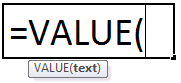
The VALUE function has only one argument, which is the required one. The VALUE formula returns a numeric value.

Where,

  • text = the text value that is to be converted into a number.

Examples to use VALUE Function in Excel

The VALUE function is a Worksheet (WS) function. As a WS function, it can be entered as a part of the formula in a worksheet cell. Refer to the examples given below to understand better.

You can download this VALUE Function Excel Template here – VALUE Function Excel Template

Example #1 – Convert TEXT into Number

VALUE function Excel Example 1

In this example, cell C2 has a VALUE formula associated with it. So, C2 is a result cell. The argument of the VALUE function is “$1,000,” the text to be converted into the number. The result is 1,000.

Example #2 – Convert the TIME of the day into a number

VALUE function Excel Example 2

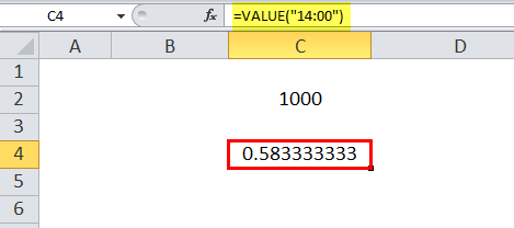
In this example, cell C4 has a VALUE formula associated with it. So, C4 is a result cell. The argument of the VALUE function is “14:00,” which is the time of the day. So, the result of converting it into a number is 0.58333.

Example #3 – Mathematical Operations

VALUE function Excel Example 3

In this example, cell C6 has a VALUE formula associated with it. So, C6 is a result cell. The argument of the VALUE function is the difference between the two values. For example, the values are “1,000” and “500”. So, the difference is 500, and the function returns the same.

Example #4 – Convert DATE into Number

VALUE Example 4

In this example, cell C8 has a VALUE formula associated with it. So, C8 is a result cell. The argument of the VALUE function is “01/12/2000,” which is the text in the date format. So, the result of converting it into the number is 36537.

Example #5 – Error in VALUE

VALUE Example 5

In this example, cell C10 has a VALUE formula associated with it. So, C10 is a result cell. Unfortunately, the argument of the VALUE function is “abc,” which is the text in an inappropriate format. Hence, we cannot process the value. As a result, #VALUE! is returned, indicating the error in value.

Example #6 – Error in NAME

VALUE Example 6

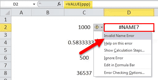
In this example, cell D2 has a VALUE formula in Excel associated with it. So, D2 is a result cell. Unfortunately, the argument of the VALUE function is ppp, which is the text in an inappropriate format, i.e., without double quotes (“). Hence, we cannot process the value.

As a result, #NAME! is returned, indicating the error is with the name provided. The same would be valid even if a valid text value is entered but not enclosed in the double quotes. E.g., VALUE (123) shall return #NAME! Error as a result.

Example #7 – Text with NEGATIVE VALUE

VALUE Example 7

In this example, cell D4 has a VALUE formula associated with it. So, D4 is a result cell. The argument of the VALUE function is “-1,” which is the text containing a negative value. As a result, the corresponding value -1 is returned by the VALUE function Excel.

Example #8 – Text with FRACTIONAL VALUE

VALUE Example 8

In this example, cell D6 has a VALUE formula in Excel associated with it. So, D6 is a result cell. The argument of the VALUE function in Excel is “0.89,” which is the text containing a fractional value. As a result, the corresponding value of 0.89 is returned by the VALUE function.

Things to Remember

  • The VALUE function converts the text into a numeric value.
  • It converts the formatted text such as date or time format into a numeric value.
  • However, Excel normally takes care of the text-to-number conversion by default. So, the VALUE function is not explicitly required.
  • It is more useful when the MS Excel data is to be made compatible with other similar spreadsheet applications.
  • It processes any numeric value less or greater than or equal to zero.
  • It processes any fractional values less or greater than or equal to zero.
  • The text entered as a parameter to be converted into the number must be enclosed within double-quotes. The #NAME! Error is returned if not done, indicating the error with the NAME entered.
  • Suppose a non-numeric text such as alphabets is entered as the parameter. In that case, the same cannot be processed by the VALUE function in Excel and returns #VALUE#VALUE! Error in Excel represents that the reference cell the user has either entered an incorrect formula or used a wrong data type (mostly numerical data). Sometimes, it is difficult to identify the kind of mistake behind this error.read more! as a result, indicating the error is with the VALUE generated.

Recommended Articles

This article has been a guide to VALUE Function in Excel. Here, we discuss the VALUE formula, how to use it, an Excel example, and a downloadable template. You may also look at these useful functions in Excel: –

  • Value Property in VBAIn VBA, the value property is usually used alongside the range method to assign a value to a range. It’s a VBA built-in expression that we can use with other functions.read more
  • Excel Shortcut Paste ValuePasting values is a common procedure that allows us to eliminate any formatting and formulas from the copied cell and paste them into the pasted cell. «Alt + E + S + V» is the shortcut key for pasting values.read more
  • NETWORKDAYS FunctionThe NETWORKDAYS function is a date and time function that determines the number of working days between two given dates  and is widely used in the fields of finance and accounting. When calculating the working days, NETWORKDAYS automatically excludes the weekend (Saturday and Sunday).read more
  • PERCENTILE Excel FunctionThe PERCENTILE function is responsible for returning the nth percentile from a supplied set of values. read more
  • Confidence Interval In ExcelConfidence Interval in excel is the range of population values that our true values lie in. read more

In this article, we will learn about how to use the VALUE function in Excel.

The VALUE function is an Excel conversion function. It converts text(date, time & currency) to a numeric value.
Syntax:

=VALUE (text)

Text: text could be date, time or currency

Note: It returns #value! error if any text (alphabets) occurs

Let’s understand this function using it an example.
Here we have different values and we will apply the same formula to the values to get the result.
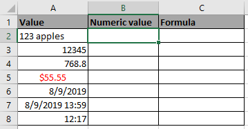
263
Use the formula

=VALUE(A2)

264
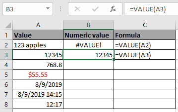
Here as you can see value function returns the #value! error where alphanumeric value occurs.
265
The VALUE function returns the numeric values corresponding to the text.

Hope you understood how to use VALUE function and referring cell in Excel. Explore more articles on Excel conversion function here. Please feel free to state your query or feedback for the above article.

Related Articles:

How to Use TEXT Function in Excel

The CHAR Function in Excel 

How to use CODE Function in Excel

Popular Articles:

How to use the VLOOKUP Function in Excel

How to use the COUNTIF function in Excel 2016

How to Use SUMIF Function in Excel

Понравилась статья? Поделить с друзьями:
  • Use two to five words to complete the second sentence using the word in bold
  • Use transform in a sentence for each word
  • Use tracking in word
  • Use too or enough and the appropriate word
  • Use too or enough and a word from the list below to complete the sentences