
Excel for Microsoft 365 Excel for Microsoft 365 for Mac Excel for the web Excel 2021 Excel 2021 for Mac Excel 2019 Excel 2019 for Mac Excel 2016 Excel 2016 for Mac Excel 2013 Excel 2010 Excel 2007 Excel for Mac 2011 Excel Starter 2010 More…Less
This article describes the formula syntax and usage of the TIME function in Microsoft Excel.
Description
Returns the decimal number for a particular time. If the cell format was General before the function was entered, the result is formatted as a date.
The decimal number returned by TIME is a value ranging from 0 (zero) to 0.99988426, representing the times from 0:00:00 (12:00:00 AM) to 23:59:59 (11:59:59 P.M.).
Syntax
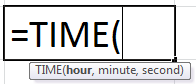
TIME(hour, minute, second)
The TIME function syntax has the following arguments:
-
Hour Required. A number from 0 (zero) to 32767 representing the hour. Any value greater than 23 will be divided by 24 and the remainder will be treated as the hour value. For example, TIME(27,0,0) = TIME(3,0,0) = .125 or 3:00 AM.
-
Minute Required. A number from 0 to 32767 representing the minute. Any value greater than 59 will be converted to hours and minutes. For example, TIME(0,750,0) = TIME(12,30,0) = .520833 or 12:30 PM.
-
Second Required. A number from 0 to 32767 representing the second. Any value greater than 59 will be converted to hours, minutes, and seconds. For example, TIME(0,0,2000) = TIME(0,33,22) = .023148 or 12:33:20 AM
Remark
Time values are a portion of a date value and represented by a decimal number (for example, 12:00 PM is represented as 0.5 because it is half of a day).
Example
Copy the example data in the following table, and paste it in cell A1 of a new Excel worksheet. For formulas to show results, select them, press F2, and then press Enter. If you need to, you can adjust the column widths to see all the data.
|
Hour |
Minute |
Second |
|---|---|---|
|
12 |
0 |
0 |
|
16 |
48 |
10 |
|
Formula |
Description |
Result |
|
=TIME(A2,B2,C2) |
Decimal part of a day, for the time specified in row 2 (12 hours, 0, minutes, 0 seconds) |
0.5 |
|
=TIME(A3,B3,C3) |
Decimal part of a day, for the time specified in row 3 (16 hours, 48 minutes, 10 seconds) |
0.7001157 |
See Also
Add or subtract time
Insert the current date and time in a cell
Date and time functions reference
Need more help?
TIME Formula in Excel
TIME is a time worksheet function in Excel that is used to make time from the arguments provided by the user. The arguments are in the following format: hours, minutes, and seconds. The range for the input for hours can be from 0-23, and for minutes it is 0-59 and similar for seconds. The method to use this function is as follows: =Time( Hours, Minutes, Seconds).
For example, TIME(0,0,3500) = 0.04050925 or 12:58:20 AM.
Table of contents
- TIME Formula in Excel
- Explanation
- Usage Notes
- How to Open the TIME Function in Excel?
- How to Use TIME in Excel Sheet?
- Example #1
- Example #2
- Example #3
- Example #4
- Example #5
- Example #6
- Example #7
- Example #8
- Excel TIME Function Errors
- Things to Remember
- TIME Function in Excel Video
- Recommended Articles
Explanation
The formula of TIME accepts the following parameters and arguments:
- hour – This can be any number between 0 and 32767, representing the hour. The point to be noted for this argument is that if the hour value is larger than 23, it will then be divided by 24. The remainder of the division will be used as the hour value. For better understanding, TIME(24,0,0) will be equal to TIME(0,0,0), TIME (25,0,0) means TIME(1,0,0) and TIME(26,0,0) will be equal to TIME(2,0,0) and so on.
- minute – This can be any number between 0 and 32767, representing the minute. For this argument, you should note that if the minute value is larger than 59, every 60 minutes will add up to 1 hour in the pre-existing hour value. For better understanding, TIME(0,60,0) will be equal to TIME(1,0,0) and TIME(0,120,0) will be equal to TIME(2,0,0) and so on.
- second – This can be any number between 0 and 32767, representing the second. For this argument, you should note that if the second value exceeds 59, then every 60 seconds will be added 1 minute to the pre-existing minute value. For better understanding, TIME(0,0,60) will be equal to TIME(0,1,0) and TIME(0,0,120) will be equal to TIME(0,2,0) and so on.
Return Value of TIME Formula:
The return value will be a numeric value between 0 and 0.999988426, which represents a particular timesheet.
Usage Notes
- The TIME in the Excel sheet is used for creating a date in serial number format from the hour, minute, and seconds components, which you specify.
- The TIME sheet creates a correct time if you have the values of the above components separately. For example, TIME(3,0,0,) is equal to 3 hours, TIME(0,3,0) is equal to 3 minutes, TIME (0,0,3) is equal to 3 seconds, and TIME(8,30,0) is equal to 8.5 hours.
- Once you get the right time, you can easily format it as per your requirements.
How to Open the TIME Function in Excel?
- You can enter the desired TIME formula in the required cell to attain a return value on the argument.
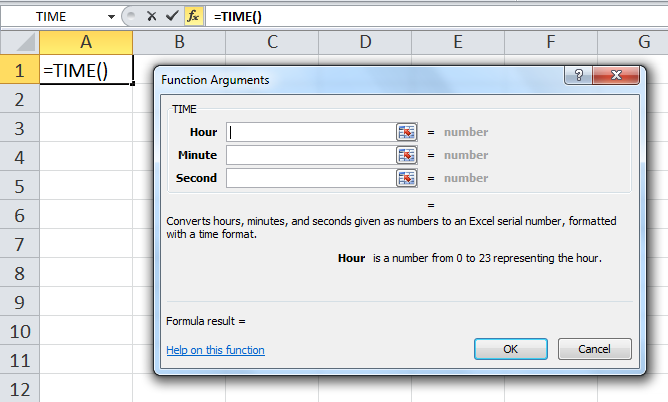
- You can manually open the TIME formula dialogue box in the spreadsheet and enter the logical values to attain a return value.
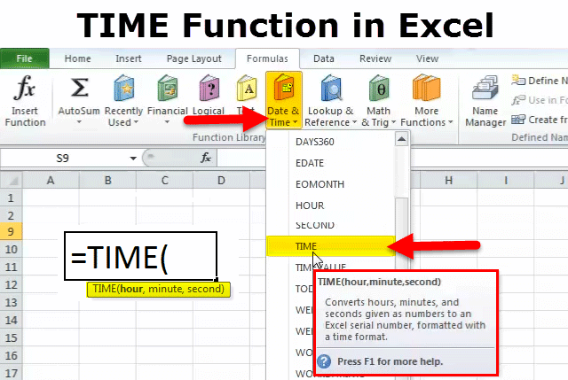
- Consider the screenshot below to see the formula of the TIME option under the DATE and TIME function in the Excel menu.

How to Use TIME in Excel Sheet?
Take a look at the below-given examples of TIME in the ExcelTo add time in Excel, the user can directly enter the time values in the hh:mm format into the cell. Remember that the time entered in the cell should not exceed 24 hours. For instance, 5.30 in the evening is written as 17:30.read more sheet. These TIME function examples will help you explore the use of the TIME function in Excel and clarify the concept of the TIME function.
You can download this TIME Function Excel Template here – TIME Function Excel Template
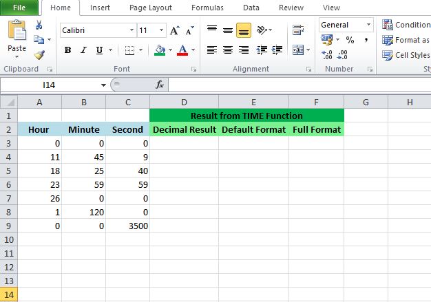
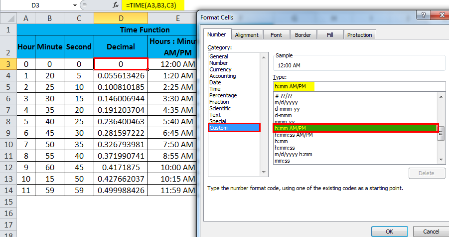
The above screenshot shows that three columns have been included: D, E, and F. These columns have different formats that offer the results generated from the TIME function. Consider the following points for better understanding.
- The column D cells are formatted with the “General” format to display the result from the TIME function in decimal values.
- The column E cells are formatted with the default h:mm AM/PM format. It is how Excel automatically formats the results once you enter the TIME formula.
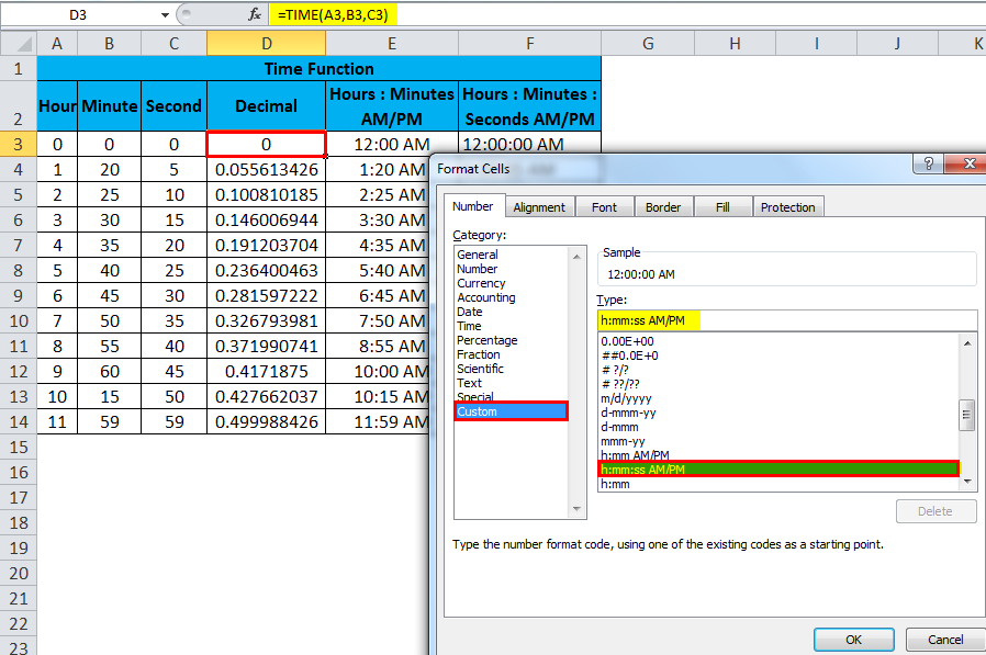
- The column F cells are formatted with h:mm:ss AM/PM custom format. It will help you see the full hours, minutes, and seconds.
Based on the above Excel spreadsheet, let us consider eight examples and see the TIME function return based on the syntax.
Note- To attain the result, you must enter the TIME formula in all three columns, D, E, and F cells.

Consider the screenshots of the above examples for a clear understanding.
Example #1

Example #2

Example #3

Example #4

Example #5

Example #6

Example #7

Example #8

Excel TIME Function Errors
If you get any error from the TIME function, it can be one of the following.
#NUM! – This kind of error occurs if the argument provided by you is evaluating a negative time; for example, if the supplied hour is less than 0.
#VALUE! – This kind of error occurs if any of the arguments are supplied by you in non-numeric.
Things to Remember
- The TIME function in Excel allows you to create time with individual hour, minute, and second components.
- The TIME in Excel is categorized under the DATE and TIME functions.
- The TIME function will return a decimal value between 0 and 0.999988426, giving an hour, minute, and second value.
- After using the TIME on Excel, once you get the right time, we can easily format it as per the requirements.
TIME Function in Excel Video
Recommended Articles
This article has been a guide to TIME Function in Excel. Here, we discuss the TIME formula in Excel and how to use the TIME function, along with Excel examples and downloadable Excel templates. You may also look at these useful functions in Excel: –
- Subtract Time in Excel FormulaFor subtraction of time values less than 24 hours, we can easily subtract using the ‘-’ operator. However, the time values that on subtraction exceed 24 hours/60 minutes/60 seconds are ignored by Excel. Therefore, we use a custom number format in such cases.read more
- Timeline ChartIn project management terms, an Excel timeline chart is also known as a Milestone chart. It is used to visually track all stages of a project and assists a project manager in delivering the project to the end-user as committed before the start of the project.read more
- DAY FunctionIn Excel, the DAY function calculates the day value from a given date. This function accepts a date as an argument and returns a two-digit numeric value as an integer value representing the given date’s day. The formula to use this function is =Edate(serial number).read more
- TODAY Excel FunctionToday function is a date and time function that is used to find out the current system date and time in excel. This function does not take any arguments and auto-updates anytime the worksheet is reopened. This function just reflects the current system date, not the time.read more
- Search For Text in ExcelExcel provides the functionality that helps you to search for text in the file. You can use Find and Search function to search for a specific text cell value and arrive at the result.read more
Reader Interactions
 Dates and times are two of the most common data types people work with in Excel, but they are also possibly the most frustrating to work with, especially if you are new to Excel and still learning. This is because Excel uses a serial number to represent the date instead of a proper month, day, or year, nevermind hours, minutes, or seconds. It’s made more complicated by the fact that dates are also days of the week, like Monday or Friday, even though Excel doesn’t explicitly store that information in the cells. Here is the definitive guide to working with dates and times in Excel…
How Excel Stores Dates
The source of most of the confusion around dates and times in Excel comes from the way that the program stores the information. You’d expect it to remember the month, the day, and the year for dates, but that’s not how it works…
Excel stores dates as a serial number that represents the number of days that have taken place since the beginning of the year 1900. This means that January 1, 1900 is really just a 1. January 2, 1900 is 2. By the time we get all the way to the present decade, the numbers have gotten pretty big… September 10, 2013 is stored as 41527.
Importantly, any date before January 1, 1900 is not recognized as a date in Excel. There are no “negative” date serial numbers on the number line.
It seems confusing, but it makes it a lot easier to add, subtract, and count days. A week from September 10, 2013 (September 17, 2013), is just 41527 + 7 days, or 41534.
How Excel Stores Times
Excel stores times using the exact same serial numbering format as with dates. Days start at midnight (12:00am or 0:00 hours). Since each hour is 1/24 of a day, it is represented as that decimal value: 0.041666…
That means that 9:00am (09:00 hours) on September 10, 2013 will be stored as 41527.375.
When a time is specified without a date, Excel stores it as if it occurred on January 0, 1900. In other words, 3:00pm (15:00 hours) is stored as 0.625. This can make doing math for time-only values (that have no date) challenging, since subtracting 6 hours (6:00) from 3:00am (03:00 hours) will become negative and count as an error: 0.125 – 0.25 = -0.125, which is displayed as #########.
Minutes and seconds in Excel work the same way as hours…
A minute is 1/60 of an hour, which is 1/24 of a day, or 1/1440 of a day in total, which calculates to 0.00069444…
A second is 1/60 of an minute, which is 1/60 of an hour, which is 1/24 of a day, or 1/86400 of a day in total, which calculates to 0.00001157407…
Working with Dates and Times
DATE() and TIME()
Serial numbers aren’t all that intuitive to use. Fortunately, Excel has a set of functions to make it easier to find and use dates and times, starting with DATE and TIME. The syntax is as follows:
=DATE(year, month, day)
=TIME(hours, minutes, seconds)
For both functions, specify the year, month, and day, or hours, minutes, and seconds as numbers. For example, September 10, 2013 can be entered as:
=DATE(2013,9,10)
It will be stored as 41527, which means that it is technically storing 12:00am on September 10, 2013.
For times, 6:00pm (18:00 hours) can be entered as:
=TIME(18,0,0)
It will be stored as 0.75, which means that it is technically storing 6:00pm on January 0, 1900.
If we want to represent a specific time and date, we can add the two functions together. For example, 6:00pm (18:00 hours) on September 10, 2013 can be entered as:
=DATE(2013,9,10)+TIME(18,0,0)
It will be calculate as 41527.75, which means Excel is storing exactly the date we want…
Additional Date and Time Setting Functions
Excel has a few additional functions to make declaring dates easier.
TODAY()
The TODAY function always returns the current date’s serial number. The TODAY function is just entered as:
=TODAY()
This article was written at 6:30pm (18:30 hours) on September 24, 2013, and the TODAY function calculated to 41541. That means that it is technically storing 12:00am on September 24, 2013.
NOW()
A similar function called NOW always returns the current date and time’s serial number. The NOW function is just entered as:
=NOW()
Again, at 6:30pm (18:30 hours) on September 24, 2013, the function calculated to 41541.77081333… NOW stores the exact time and date, down to the second.
EDATE() and EOMONTH()
The EDATE function gives the date the specified number of months away from the input date. The EOMONTH function gives the date of the last day of the month. It can do so for the current month or a number of months in the future or the past. The syntax for each is as follows:
=EDATE(start_date, months)
=EOMONTH(start_date, months)
The start_date can be any date-formatted cell reference or date serial number.
The months field can be any number, though only the integer value will be used (e.g. it treats 2.8 as 2).
The EDATE and EOMONTH functions strip the time value from the date. For example, For example, if cell A1 stores September 10, 2013, we can get the value 2 months ahead as follows:
=EDATE(A1,2)
Returns 12:00am (0:00 hours) on November 10, 2013, or 41588. This function works even though the months have different numbers of days (September and November have 30, October has 31).
=EOMONTH(A1,2)
Returns 12:00am (0:00 hours) on November 30, 2013, or 41588. Again, this function works even though the months have different numbers of days.
WORKDAY()
Occasionally, it may be useful to count ahead based on work-days (Monday-Friday) instead of all 7 days of the week… For that, Excel has provided WORKDAY. The syntax for WORKDAY is as follows:
=WORKDAY(start_date, days, [holidays])
The start_date is as above.
The days input is the number of workdays ahead (or behind) of the present day you would like to move.
The [holidays] input is optional, but lets you disqualify specific days (like Thanksgiving or Christmas, for example), which might otherwise fall during the work week. These are date serial numbers provided in an array bounded by brackets: { }. To specify multiple holidays, the dates must be held in cells – it is not possible to put multiple DATE functions in an array.
For example, let’s find the date 6 work days before 6:00pm (18:00 hours) on September 10, 2013 (stored in cell A1). Monday, September 2nd is Labor Day, so let’s include that as a holiday:
=WORKDAY(A1,-6,DATE(2013,9,2))
Returns 12:00am (0:00 hours) on August 30, 2013, or 41516. (Note that the function strips the time portion of the date.)
WORKDAY.INTL() (Excel 2010 and newer)
For newer versions of Excel (2010 and later), there is another version of WORKDAY called WORKDAY.INTL. WORKDAY.INTL works just like WORKDAY, but it adds the ability to customize the definition of the “weekend”. The syntax for WORKDAY.INTL is as follows:
=WORKDAY.INTL(start_date, days, [weekend], [holidays])
The start_date, days, and [holidays] inputs work just like the normal WORKDAY function.
The [weekend] input has the following options:
Retrieving Dates in Excel
DAY(), MONTH(), and YEAR()
Now we know how define dates, but we still need to be able to work with them. Serial numbers don’t make it easy to extract months, years, and days, nevermind hours, minutes, and seconds. That’s why Excel has specific functions for pulling out each of these values. For working with the calendar, there is DAY, MONTH, and YEAR. The syntax is simple:
=DAY(serial_number)
=MONTH(serial_number)
=YEAR(serial_number)
The serial_number in each can be any date-formatted cell reference. For example, if cell A1 stores September 10, 2013, we can use each of the formulas in turn:
=DAY(A1)
Returns 10 as a numeric value.
=MONTH(A1)
Returns 9 as a numeric value.
=YEAR(A1)
Returns 2013 as a numeric value.
We could have also given the direct serial number for September 10, 2013:
=DAY(41527)
Returns 10 as a numeric value.
Retrieving Times in Excel
HOUR(), MINUTE(), and SECOND()
For times, the process is very similar. Excel has function to retrieve the hours, minutes, and seconds from a time stamp, conveniently named HOUR, MINUTE, and SECOND. The syntax is identical:
=HOUR(serial_number)
=MINUTE(serial_number)
=SECOND(serial_number)
The serial_number in each can be any time/date-formatted cell reference. For example, if A1 stores 6:15:30pm (18:15 hours, 30 seconds) on September 10, 2013, we can use each of the formulas in turn:
=HOUR(A1)
Returns 18 as a numeric value.
=MINUTE(A1)
Returns 15 as a numeric value.
=SECOND(A1)
Returns 30 as a numeric value.
We could have also given the direct serial number for 6:15:30pm (18:15 hours, 30 seconds) on September 10, 2013:
=SECOND(41527.7607638889)
Returns 30 as a numeric value.
Additional Date Retrieving Functions
WEEKDAY() and WEEKNUM()
Dates don’t just have month and year information. They also encode indirect information… September 10, 2013 happens to also be a Tuesday. Excel has a few of functions to work with the week aspect of dates: WEEKDAY and WEEKNUM. The syntax is as follows:
=WEEKDAY(serial_number, [return_type])
=WEEKNUM(serial_number, [return_type])
The serial_number in each can be any date-formatted cell reference. Since [return_type] is optional, each function assumes that each week starts on Sunday. If cell A1 stores September 10, 2013 (a Tuesday), we can use each of the formulas in turn:
=WEEKDAY(A1)
Returns 3, since Tuesday is the 3rd day of a week that starts on Sunday.
=WEEKNUM(A1)
Returns 37, since September 10, 2013 is in the 37th week of 2013, when you start counting weeks from Sunday.
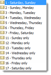
The [return_type] allows you to specify a different default week arrangement. You could let the week start on Monday and run until Sunday, or Saturday until Friday, for example. Excel is annoying, however, and makes the entry different for WEEKDAY and WEEKNUM. The full list of options for WEEKDAY is as follows:
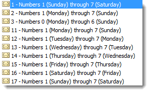
Options 2 and 11 are functionally the same – the first is just there for backwards compatibility with earlier versions of Excel.
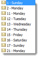
The full list of options for WEEKNUM is as follows:
Counting and Tracking Dates
Dates can be added and subtracted like normal numbers because they’re stored as serial numbers. That lets you count the days between two different dates. Sometimes, though, you need to count by a different metric.
NETWORKDAYS()
Above, we learned about WORKDAY, which lets you move back and forth a set number of workdays, ignoring weekends and holidays. But what if you need to measure the number of workdays between two dates? For that, Excel provides NETWORKDAYS. The formula syntax is as follows:
=NETWORKDAYS(start_date, end_date, [holidays])
The start_date and end_date can be any date-formatted cell reference.
The [holidays] input is optional, but lets you disqualify specific days (like Thanksgiving or Christmas, for example), which might otherwise fall during the work week. These are date serial numbers provided in an array bounded by brackets: { }. To specify multiple holidays, the dates must be held in cells – it is not possible to put multiple DATE functions in an array.
For example, if A1 contains 6:00pm (18:00 hours) on September 10, 2013 and B1 contains 9:00am (9:00 hours) on December 2, 2013, we can use NETWORKDAYS to find the number of workdays between the two dates.
Let’s exclude Columbus Day (October 14, 2013), Veterans Day (November 11, 2013), and Thanksgiving Day (November 28, 2013) as holidays. To do so, we have to store those dates in other cells. Let’s put them in C1, C2, and C3:
=DATE(2013,10,14)
=DATE(2013,11,11)
=DATE(2013,11,28)
Now, we can combine them in the function:
=NETWORKDAYS(A1,B1,C1:C3)
The function returns 57 as a numeric value.
NETWORKDAYS.INTL() (Excel 2010 and newer)
For newer versions of Excel (2010 and later), there is another version of NETWORKDAYS called NETWORKDAYS.INTL. NETWORKDAYS.INTL works just like NETWORKDAYS, but it adds the ability to customize the definition of the “weekend”. The syntax for NETWORKDAYS.INTL is as follows:
=NETWORKDAYS.INTL(start_date, end_date, [weekend], [holidays])
The start_date, end_date, and [holidays] inputs work just like the normal WORKDAY function.
The [weekend] input has the following options:
YEARFRAC()
Sometimes it’s useful to measure how much time has passed in years, but subtracting the YEAR function will only round down to the nearest full year. YEARFRAC takes two dates and provides the portion of the year between them. The syntax is as follows:
=YEARFRAC(start_date, end_date, [basis])
The start_date and end_date can be any date-formatted cell reference.
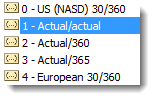
The [basis] input is optional, but lets you specify the “rules” for measuring the difference. Most of the time, you’ll want to use option 1, but here is the full list:
 For example, if A1 contains September 10, 2013 and B1 contains December 2, 2013, we can use YEARFRAC to find the decimal portion of a year between the two dates:
=YEARFRAC(A1,B1,1)
Returns 0.227397260273973.
DATEDIF() (Undocumented Function)
The YEARFRAC function gives you the difference between dates as a fraction of a year, but sometimes you need more control. There is a powerful hidden function in Excel called DATEDIF that can do much more. It can tell you the number of years, months, or days between two dates. It can also track based on only partial inputs, ignoring years or months when calculating days. The syntax for DATEDIF is as follows:
=DATEDIF(start_date, end_date, unit)
The start_date and end_date can be any date-formatted cell reference.
The unit input asks you to specify a string that represents the type of output you want. This is slightly cumbersome, since you must wrap the input in quotes (” “).
For example, if A1 contains September 10, 2012 and B1 contains December 2, 2013, we can use DATEDIF to find the number of full years between the two dates:
=DATEDIF(A1,B1,"Y")
Returns 1 as a numeric value.
Using the same start_date and end_date inputs, here are the output possibilities for DATEDIF using different unit parameters:
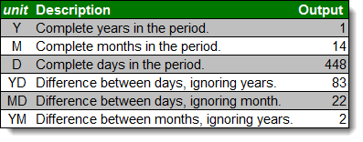
Every time, the unit must be put in quotes (e.g. “Y” or “MD”).
Converting Dates and Times from Text
DATEVALUE() and TIMEVALUE()
All of the above functions work perfectly with date-formatted serial numbers in Excel. Unfortunately, dates and times are often imported into worksheets as text. Most of the assorted functions like MONTH and HOUR are reasonably intelligent about converting on the fly. Occasionally it’s useful to build a date value through concatenation. The two functions Excel provides for this purpose are DATEVALUE and TIMEVALUE. The syntax for each is as follows:
=DATEVALUE(date_text)
=TIMEVALUE(time_text)
The date_text and time_text accept any text string that looks like a date or time.
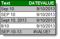
This is how DATEVALUE responds to various date_text inputs:
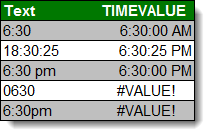
This is how TIMEVALUE responds to various time_text inputs:
Converting Dates and Times to Text
TEXT()
Getting data converted to dates and times is great, but you may also need to get it back out. Sometimes, you need a special format. Other times, you need to look for a date in a text string, and have to match using string tools like FIND and SEARCH. There is one master function for converting dates and times to text strings in Excel, called TEXT. The syntax for TEXT is as follows:
=TEXT(value, format_text)
The value can be any date or time-formatted cell reference.
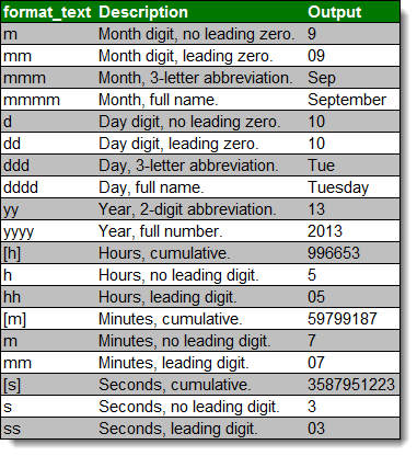
The format_text input has a large number of options, summarized here:
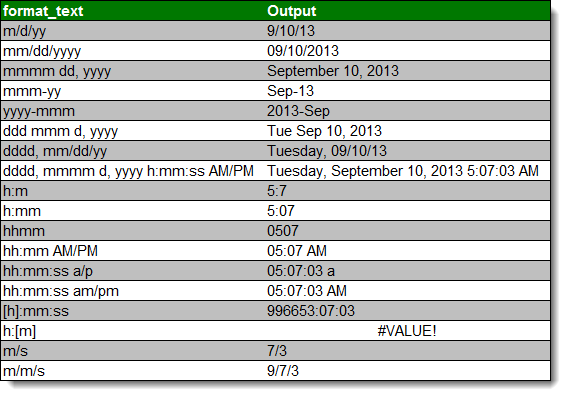
The outputs can be combined with simple formatting characters to produce standard date formats. Using the date 5:07:03am (05:07 hours, 3 seconds) on September 10, 2013, here are examples of possible outputs:
A Common Problem
One issue people frequently run into is that Excel occasionally misinterprets text fields as dates. An example is here:
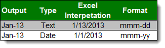
Be careful when entering dates, especially if you are importing from other data sources, to make sure that your “Jan-13” is being stored as January 1, 2013 and not January 13, 2013!
Get the latest Excel tips and tricks by joining the newsletter!
 Andrew Roberts has been solving business problems with Microsoft Excel for over a decade. Excel Tactics is dedicated to helping you master it.
Join the newsletter to stay on top of the latest articles. Sign up and you’ll get a free guide with 10 time-saving keyboard shortcuts!
Other posts in this series…
TIME in Excel (Table of Contents)
- TIME in Excel
- TIME Formula in Excel
- How to Use TIME Function in Excel?
TIME in Excel
Time function in excel is just another time function that returns HHMM AM/PM Format time. We just need to feed Hour, Minute and Second as per our requirement, and the time function will exactly return the same value in AM and PM details. One thing we need to note, that if the Hours’ range is less than and equal to 12, then the time which we get would be in AM and post 12; the time would be in PM till 11:59 in the clock.
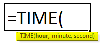
TIME Formula in Excel:
The Formula for the TIME Function in Excel is given below.
Arguments:
- Hour: If the hour value is greater than 23, it will be divided by 24, and the remainder will be used as the hour value. This means that TIME(24,0,0) is equal to TIME(0,0,0) and TIME(25,0,0) is equal to TIME(1,0,0).
- Minute: If the minute value is greater than 59, then every 60 minutes will add 1 hour to the hour value. This means that TIME(0,60,0) is equal to TIME(1,0,0) and TIME(0,120,0) is equal to TIME(2,0,0).
- Second: If the second value is greater than 59, then every 60 seconds will add 1 minute to the minute value. This means that TIME(0,0,60) is equal to TIME(0,1,0) and TIME(0,0,120) is equal to TIME(0,2,0)
Steps to Open TIME Function in Excel
We can enter the time in a normal time format so that Excel will take the default one by default. Please follow the below step by step procedure. Choose time format in the Format Cells dialog; you may have noticed that one of the formats begins with an asterisk (*). This is the default time format in your Excel.
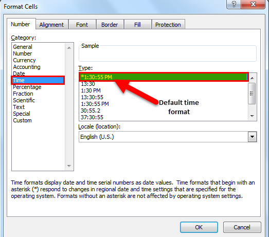
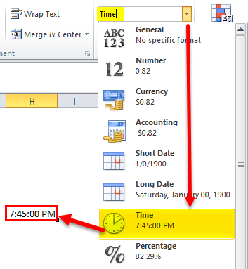
To quickly apply the default Excel time format to the selected cell or a range of cells, click the drop-down arrow in the Number group, on the Home tab, and select Time.
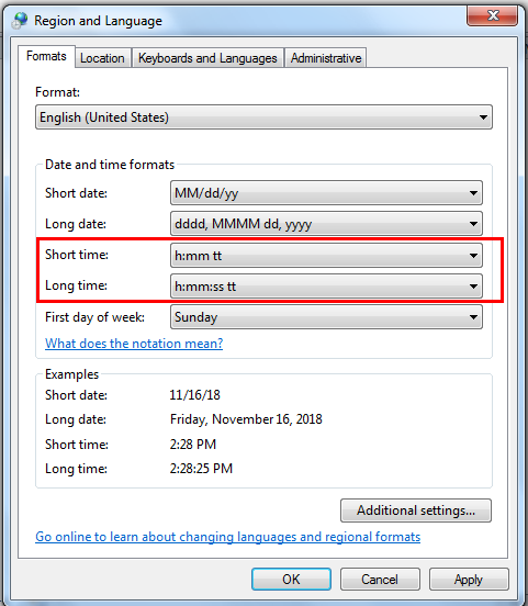
To change the default time format, go to the Control Panel and click Region and Language. If in your Control panel opens in Category view, click Clock, Language, and Region > Region and Language > Change the date, time, or number format.
NOTE: When creating a new Excel time format or modifying an existing one, please remember that regardless of how you’ve chosen to display time in a cell, Excel always internally stores times the same way – as decimal numbers.
How to Use TIME Function in Excel?
This TIME Function in Excel is very simple easy to use. Let us now see how to use the TIME Function in Excel with the help of some examples.
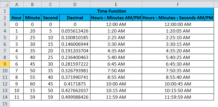
In the above example, we have three columns Decimal, Hours: Minutes, Hours: Minutes: Seconds with three different format which show the TIME function result.
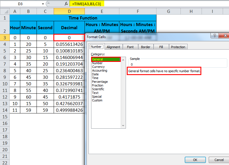
Decimal
We have used the same TIME Function in this format and displayed used General (Decimal) format. In order to convert into a decimal format, right-click and choose format cells and then choose general.
Hours: Minutes
The second format we have used is Hours & Minutes; in order to display in the above format, right-click and choose format cell there, we will find the custom option where we will get a variety of hours formats to choose the appropriate format for H:MM AM/PM.
Hours: Minutes: Seconds:
The third format is Hours: Minutes: Seconds, where we have used the same TIME function to display it. In order to create a right-click and choose format cell there, we will find the custom option where we will get a variety of hours formats to choose the appropriate format for H:M:SS AM/PM.
This time function can be useful in all productivity scenarios. Remember that the TIME function will “roll over” back to zero when values exceed 24 hours, wherein the advanced MOD function can be exactly used to differentiate AM/PM, and this MOD function will take care of the negative numbers problem. MOD will “flip” negative values to the required positive values.
For example, if the employee works for 9 hours and he extended his Overtime for another 5 hours. In this scenario, if we want to find the start time and end time, we can use the MOD function to calculate how many hours an employee has been worked.
What is MOD Function?
The MOD function is defined as “Returns the remainder after a number is divided by a divisor.”
The Formula for MOD Function:
=MOD(number, divisor)
To calculate the date and time difference in Excel is a common task. Unfortunately, depending on requirements, it is also not always a simple one.
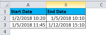
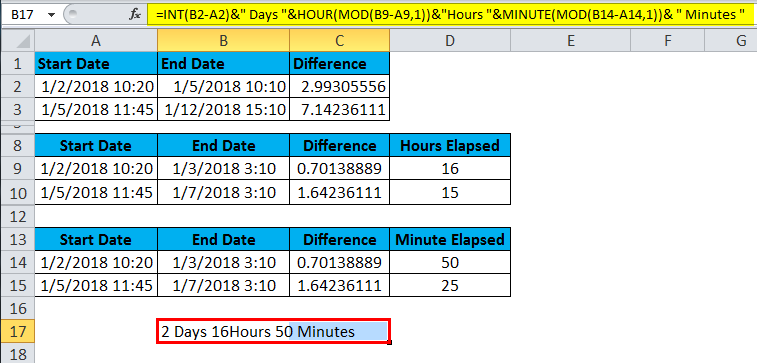
In the below example where column A contains a start date and time, and column B an end date and time. We wish to calculate the elapsed time in days, hours and minutes, e.g. 11 days 4 hours 9 minutes.
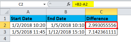
There are multiple ways of calculating the date and time difference in Excel. In this scenario, we will need to get a little clever. As you may well know, date and time values are stored as numbers in Excel. For example, the 05/01/2018 10:10 is stored as 2.993055556.
Therefore, if I write the formula as =B2-A2.
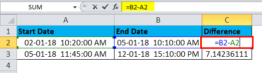
Then the result is returned as 2.993056.
To return a result that makes sense to us, we will tackle the date and time parts of the cell separately.
Calculating the Number of Days Difference
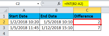
To work with just the date part of the cell, we will use the INT function. This function rounds a value down to the nearest integer. So if we write the function below, this will return only the integer part of the date difference, which is the number of days.
=INT (B2-A2)
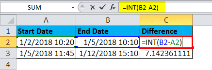
Then the result is returned as 2.
Calculating the Elapsed Hours and Minutes
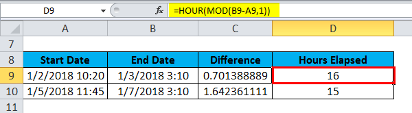
We now need to work on the number of hours and minutes, which is the decimal part. To return only the decimal part of the B9-A9 formula, we will use the MOD function. This function returns the remainder after a number is divided by a divisor.
We will use it to divide the B9-A9 formula by 1 so that it returns to the remainder as the decimal part. We will then use the HOUR and MINUTE functions to return the hours and minutes from this decimal value.
So the formula below returns the number of hours elapsed.
=HOUR(MOD(B9-A9,1))
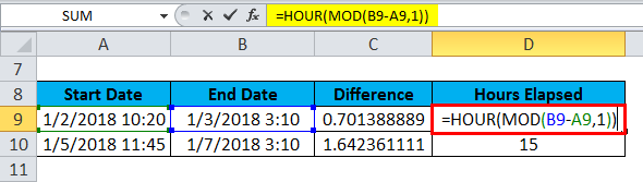
Then the result is returned as 16.
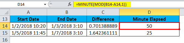
And this returns the number of minutes elapsed.
=MINUTE(MOD(B14-A14,1))
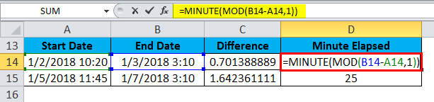
Then the result is returned as 50.
A formula for Elapsed Time in Days, Hours and Minutes
Finally, we need to put this all together as one Excel formula. We can use the ampersand (&) to concatenate the different parts of the formula. You can construct the result to look however you want. For example, the formula below would return the result as 2 days, 23 hours and 50 minutes.
=INT(B2-A2)&” Days “&HOUR(MOD(B9-A9,1))&” Hours “&MINUTE(MOD(B14-A14,1))& ” Minutes ”
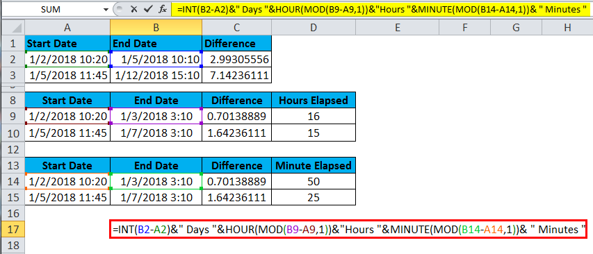
It will return the result as 2 days, 16 hours and 50 minutes.
Recommended Articles
This has been a guide to TIME in Excel. Here we discuss the TIME Formula in Excel and how to use TIME Function in Excel along with excel example and downloadable excel templates. You may also look at these useful functions in excel –
- MID Function in Excel
- Time Difference in Excel
- Excel Sum Time
- Excel Timesheet Template
Since dates and times are stored as numbers in the back end in Excel, you can easily use simple arithmetic operations and formulas on the date and time values.
For example, you can add two different time values or date values or you can calculate the time difference between two given dates/times.
In this tutorial, I will show you a couple of ways to perform calculations using time in Excel (such as calculating the time difference, adding or subtracting time, showing time in different formats, and doing a sum of time values)
How Excel Handles Date and Time?
As I mentioned, dates and times are stored as numbers in a cell in Excel. A whole number represents a complete day and the decimal part of a number would represent the part of the day (which can be converted into hours, minutes, and seconds values)
For example, the value 1 represents 01 Jan 1900 in Excel, which is the starting point from which Excel starts considering the dates.
So, 2 would mean 02 Jan 1990, 3 would mean 03 Jan 1900 and so on, and 44197 would mean 01 Jan 2021.
Note: Excel for Windows and Excel for Mac follow different starting dates. 1 in Excel for Windows would mean 1 Jan 1900 and 1 in Excel for Mac would mean 1 Jan 1904
If there are any digits after a decimal point in these numbers, Excel would consider those as part of the day and it can be converted into hours, minutes, and seconds.
For example, 44197.5 would mean 01 Jan 2021 12:00:00 PM.

So if you’re working with time values in Excel, you would essentially be working with the decimal portion of a number.
And Excel gives you the flexibility to convert that decimal portion into different formats such as hours only, minutes only, seconds only, or a combination of hours, minutes, and seconds
Now that you understand how time is stored in Excel, let’s have a look at some examples of how to calculate the time difference between two different dates or times in Excel
Formulas to Calculating Time Difference Between Two Times
In many cases, all you want to do is find out the total time that has elapsed between the two-time values (such as in the case of a timesheet that has the In-time and the Out-time).
The method you choose would depend on how the time is mentioned in a cell and in what format you want the result.
Let’s have a look at a couple of examples
Simple Subtraction of Calculate Time Difference in Excel
Since time is stored as a number in Excel, find the difference between 2 time values, you can easily subtract the start time from the end time.
End Time – Start Time
The result of the subtraction would also be a decimal value that would represent the time that has elapsed between the two time-values.
Below is an example where I have the start and the end time and I have calculated the time difference with a simple subtraction.

There is a possibility that your results are shown in the time format (instead of decimals or in hours/minutes values). In our above example, the result in cell C2 shows 09:30 AM instead of 9.5.
That’s perfectly fine as Excel tries to copy the format from the adjacent column.
To convert this into a decimal, change the format of the cells to General (the option is in the Home tab in the Numbers group)
Once you have the result, you can format it in different ways. For example, you can show the value in hours only or minutes only or a combination of hours, minutes, and seconds.
Below are the different formats you can use:
| Format | What it Does |
| h | Shows only the hours elapsed between the two dates |
| hh | Shows hours in double-digit (such as 04 or 12) |
| hh:mm | Shows hours and minutes elapsed between the two dates, such as 10:20 |
| hh:mm:ss | Shows hours, minutes, and seconds elapsed between the two dates, such as 10:20:36 |
And if you’re wondering where and how to apply these custom date formats, follow the below steps:
- Select the cells where you want to apply the date format
- Hold the Control key and press the 1 key (or Command + 1 if using Mac)
- In the Format Cells dialog box that opens, click on the Number tab (if not selected already)

- In the left pane, click on Custom
- Enter any of the desired format code in the Type field (in this example, I am using hh:mm:ss)
- Click OK


The above steps would change the formatting and show you the value based on the format.

Note that custom number formatting does not change the value in the cell. It only changes the way a value is being displayed. So, I can choose to only show the hour value in a cell, while it would still have the original value.
Pro tip: If the total number of hours exceeds 24 hours, use the following custom number format instead: [hh]:mm:ss
Calculate the Time Difference in Hours, Minutes, or Seconds
When you subtract the time values, Excel returns a decimal number that represents the resulting time difference.
Since every whole number represents one day, the decimal part of the number would represent that much part of the day which can easily be converted into hours or minutes, or seconds.
Calculating Time Difference in Hours
Suppose you have the dataset as shown below and you want to calculate the number of hours between the two-time values

Below is the formula that will give you the time difference in hours:
=(B2-A2)*24
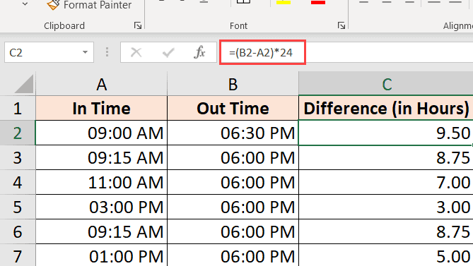
The above formula will give you the total number of hours elapsed between the two-time values.
Sometimes, Excel tries to be helpful and will give you the result in time format as well (as shown below).

You can easily convert this into Number format by clicking on the Home tab, and in the Number group, selecting Number as the format.

If you only want to return the total number of hours elapsed between the two times (without any decimal part), use the below formula:
=INT((B2-A2)*24)

Note: This formula only works when both the time values are of the same day. If the day changes (where one of the time values is of another date and the second one of another date), This formula will give wrong results. Have a look at the section where I cover the formula to calculate the time difference when the date changes later in this tutorial.
Calculating Time Difference in Minutes
To calculate the time difference in minutes, you need to multiply the resulting value by the total number of minutes in a day (which is 1440 or 24*60).
Suppose you have a data set as shown below and you want to calculate the total number of minutes elapsed between the start and the end date.
Below is the formula that will do that:
=(B2-A2)*24*60

Calculating Time Difference in Seconds
To calculate the time difference in seconds, you need to multiply the resulting value by the total number of seconds in a day (which is or 24*60*60 or 86400).
Suppose you have a data set as shown below and you want to calculate the total number of seconds that have elapsed between the start and end date.
Below is the formula that will do that:
=(B2-A2)*24*60*60

Calculating time difference with the TEXT function
Another easy way to quickly get the time difference without worrying about changing the format is to use the TEXT function.
The TEXT function allows you to specify the format right within the formula.
=TEXT(End Date - Start Date, Format)
The first argument is the calculation you want to do, and the second argument is the format in which you want to show the result of the calculation.
Suppose you have a dataset as shown below and you want to calculate the time difference between the two times.
Here are some formulas that will give you the result with different formats
Show only the number of hours:
=TEXT(B2-A2,"hh")

The above formula will only give you the result that shows the numbers of hours elapsed between the two-time values. If your result is 9 hours and 30 minutes, it will still show you 9 only.
Show the number of total minutes
=TEXT(B2-A2,"[mm]")

Show the number of total seconds
=TEXT(B2-A2,"[ss]")

Show Hours and Minutes
=TEXT(B2-A2,"[hh]:mm")

Show Hours, Minutes, and Seconds
=TEXT(B2-A2,"hh:mm:ss")

If you’re wondering what’s the difference between hh and [hh] in the format (or mm and [mm]), when you use the square brackets, it would give you the total number of hours between the two dates, even if the hour value is higher than 24. So if you subtract two date values where the difference is more than24 hours, using [hh] will give you the total number of hours and hh will only give you the hours elapsed on the day of the end date.
Get the Time Difference in One-Unit (Hours/Minutes) and Ignore Others
If you want to calculate the time difference between the two time-values in only the number of hours or minutes or seconds, then you can use the dedicated HOUR, MINUTE, or SECOND function.
Each of these functions takes one single argument, which is the time value, and returns the specified time unit.
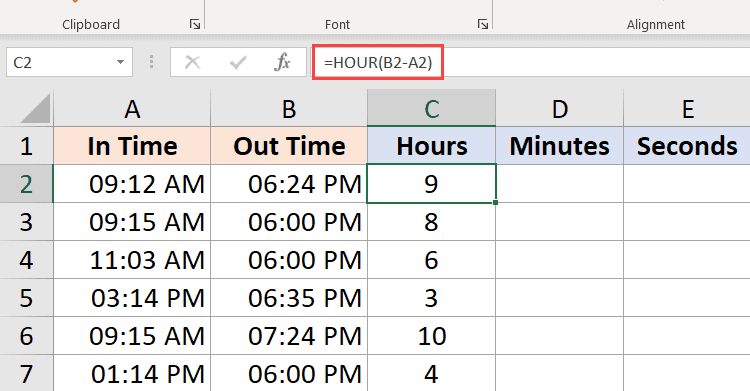
Suppose you have a data set as shown below, and you want to calculate the total number of hours minutes, and seconds that have elapsed between these two times.

Below are the formulas to do this:
Calculating Hours Elapsed Between two times
=HOUR(B2-A2)
Calculating Minutes from the time value result (excluding the completed hours)
=MINUTE(B2-A2)

Calculating Seconds from the time value result (excluding the completed hours and minutes)
=SECOND(B2-A2)

A couple of things that you need to know when working with these HOURS, MINUTE, and SECOND formulas:
- The difference between the end time and the start time cannot be negative (which is often the case when the date changes). In such cases, these formulas would return a #NUM! error
- These formulas only use the time portion of the resulting time value (and ignore the day portion). So if the difference in the end time and the start time is 2 Days, 10 Hours, 32 Minutes, and 44 Seconds, the HOUR formula will give 10, the MINUTE formula will give 32, and the SECOND formula will give 44
Calculate elapsed time Till Now (from the start time)
If you want to calculate the total time that has elapsed between the start time and the current time, you can use the NOW formula instead of the End time.
NOW function returns the current date and the time in the cell in which it is used. It’s one of those functions that does not take any input argument.
So, if you want to calculate the total time that has elapsed between the start time and the current time, you can use the below formula:
=NOW() - Start Time
Below is an example where I have the start times in column A, and the time elapsed till now in column B.

If the difference in time between the start date and time and the current time is more than 24 hours, then you can format the result to show the day as well as the time portion.
You can do that by using the below TEXT formula:
=TEXT(NOW()-A2,"dd hh:ss:mm")
You can also achieve the same thing by changing the custom formatting of the cell (as covered earlier in this tutorial) so that it shows the day as well as the time portion.
In case your start time only has the time portion, then Excel would consider it as the time on 1st January 1990.
In this case, if you use the NOW function to calculate the time elapsed till now, it is going to give you the wrong result (as the resulting value would also have the total days that have elapsed since 1st Jan 1990).
In such a case, you can use the below formula:
=NOW()- INT(NOW())-A2
The above formula uses the INT function to remove the day portion from the value returned by the now function, and this is then used to calculate the time difference.
Note that NOW is a volatile function that updates whenever there is a change in the worksheet, but it does not update in real-time
Calculate Time When Date Changes (calculate and display negative times in Excel)
The methods covered so far work well if your end time is later than the start time.
But the problem arises when your end time is lower than the start time. This often happens when you are filling timesheets where you only enter the time and not the entire date and time.
In such cases, if you’re working in a one night shift and the date changes, there is a possibility that your end time would be earlier than your start time.
For example, if you start your work at 6:00 PM in the evening, and complete your work & time out at 9:00 AM in the morning.
If you only working with time values, then subtracting the start time from the end time is going to give you a negative value of 9 hours (9 – 18).
And Excel cannot handle negative time values (and for that matter nor can humans, unless you can time travel)
In such cases, you need a way to figure out that the day has changed and the calculation should be done accordingly.
Thankfully, there is a really easy fix for this.
Suppose you have a dataset as shown below, where I have the start time and the end time.

As you would notice that sometimes the start time is in the evening and the end time is in the morning (which indicates that this was an overnight shift and the day has changed).
If I use the below formula to calculate the time difference, it will show me the hash signs in the cells where the result is a negative value (highlighted in yellow in the below image).
=B2-A2

Here is an IF formula that whether the time difference value is negative or not, and in case it is negative then it returns the right result
=IF((B2-A2)<0,1-(A2-B2),(B2-A2))

While this works well in most cases, it still falls short in case the start time and the end time is more than 24 hours apart. For example, someone signs in at 9:00 AM on day 1 and sign-out at 11:00 AM on day 2.
Since this is more than 24 hours, there is no way to know whether the person has signed out after 2 hours or after 26 hours.
While the best way to tackle this would be to make sure that the entries include the date as well as the time, but if it’s just the time that you’re working with, then the above formula should take care of most of the issues (considering it’s unlikely for anyone to work for more than 24 hours)
Adding/ Subtracting Time in Excel
So far, we have seen examples where we had the start and the end time, and we needed to find the time difference.
Excel also allows you to easily add or subtract a fixed time value from the existing date and time value.
For example, let’s say you have a list of queued tasks where each task takes the specified time, and you want to know when each task will end.
In such a case, you can easily add the time that each task is going to take to the start time to know at what time is the task expected to be completed.
Since Excel stores date and time values as numbers, you have to ensure that the time you are trying to add abides by the format that Excel already follows.
For example, if you add 1 to a date in Excel, it is going to give you the next date. This is because 1 represents an entire day in Excel (which is equal to 24 hours).
So if you want to add 1 hour to an existing time value, you cannot go ahead and simply add 1 to it. you have to make sure that you convert that hour value into the decimal portion that represents one hour. and the same goes for adding minutes and seconds.
Using the TIME Function
Time function in Excel takes the hour value, the minute value, and the seconds value and converts it into a decimal number that represents this time.
For example, if I want to add 4 hours to an existing time, I can use the below formula:
=Start Time + TIME(4,0,0)

This is useful if you know how many hours, minutes, and seconds you want to add to an existing time and simply use the TIME function without worrying about the correct conversion of the time into a decimal value.
Also, note that the TIME function will only consider the integer part of the hour, minute, and seconds value that you input. For example, if I use 5.5 hours in the TIME function it would only add five hours and ignore the decimal part.
Also, note that the TIME function can only add values that are less than 24 hours. If your hour value is more than 24, this would give you an incorrect result.
And the same goes with the minutes and the second’s part where the function will only consider values that are less than 60 minutes and 60 seconds
Just like I have added time using the TIME function, you can also subtract time. Just change the + sign to a negative sign in the above formulas
Using Basic Arithmetic
When the time function is easy and convenient to use, it does come with a few restrictions (as covered above).
If you want more control, you can use the arithmetic method that I’ll cover here.
The concept is simple – convert the time value into a decimal value that represents the portion of the day, and then you can add it to any time value in Excel.
For example, if you want to add 24 hours to an existing time value, you can use the below formula:
=Start_time + 24/24
This just means that I’m adding one day to the existing time value.
Now taking the same concept forward let’s say you want to add 30 hours to a time value, you can use the below formula:
=Start_time + 30/24
The above formula does the same thing, where the integer part of the (30/24) would represent the total number of days in the time that you want to add, and the decimal part would represent the hours/minutes/seconds
Similarly, if you have a specific number of minutes that you want to add to a time value then you can use the below formula:
=Start_time + (Minutes to Add)/24*60
And if you have the number of seconds that you want to add, then you can use the below formula:
=Start_time + (Minutes to Add)/24*60*60
While this method is not as easy as using the time function, I find it a lot better because it works in all situations and follows the same concept. unlike the time function, you don’t have to worry about whether the time that you want to add is less than 24 hours or more than 24 hours
You can follow the same concept while subtracting time as well. Just change the + to a negative sign in the formulas above
How to SUM time in Excel
Sometimes you may want to quickly add up all the time values in Excel. Adding multiple time values in Excel is quite straightforward (all it takes is a simple SUM formula)
But there are a few things you need to know when you add time in Excel, specifically the cell format that is going to show you the result.
Let’s have a look at an example.
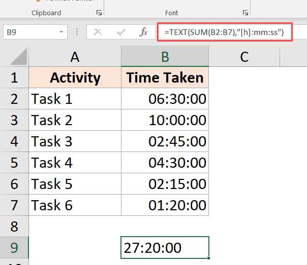
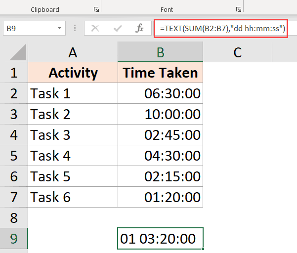
Below I have a list of tasks along with the time each task will take in column B, and I want to quickly add these times and know the total time it is going to take for all these tasks.

In cell B9, I have used a simple SUM formula to calculate the total time all these tasks are going to take, and it gives me the value as 18:30 (which means that it is going to take 18 hours and 20 minutes to complete all these tasks)

All good so far!
How to SUM over 24 hours in Excel
Now see what happens when I change at the time it is going to take Task 2 to complete from 1 hour to 10 hours.

The result now says 03:20, which means that it should take 3 hours and 20 minutes to complete all these tasks.
This is incorrect (obviously)
The problem here is not Excel messing up. The problem here is that the cell is formatted in such a way that it will only show you the time portion of the resulting value.
And since the resulting value here is more than 24 hours, Excel decided to convert the 24 hours part into a day remove it from the value that is shown to the user, and only display the remaining hours, minutes, and seconds.
This, thankfully, has an easy fix.
All you need to do is change the cell format to force it to show hours even if it exceeds 24 hours.
Below are some formats that you can use:
| Format | Expected Result |
| [h]:mm | 28:30 |
| [m]:ss | 1710:00 |
| d “D” hh:mm | 1 D 04:30 |
| d “D” hh “Min” ss “Sec” | 1 D 04 Min 00 Sec |
| d “Day” hh “Minute” ss “Seconds” | 1 Day 04 Minute 00 Seconds |
You can change the format by going to the format cells dialog box and applying the custom format, or use the TEXT function and use any of the above formats in the formula itself
You can use the below the TEXT formula to show the time, even when it’s more than 24 hours:
=TEXT(SUM(B2:B7),"[h]:mm:ss")
or the below formula if you want to convert the hours exceeding 24 hours to days:
=TEXT(SUM(B2:B7),"dd hh:mm:ss")
Results Showing Hash (###) Instead of Date/Time (Reasons + Fix)
In some cases, you may find that instead of showing you the time value, Excel is displaying the hash symbols in the cell.
Here are some possible reasons and the ways to fix these:
The column is not wide enough
When a cell doesn’t have enough space to show the complete date, it may show the hash symbols.
It has an easy fix – change the column width and make it wider.
Negative Date Value
A date or time value cannot be negative in Excel. in case you are calculating the time difference and it turns out to be negative, Excel will show you hash symbols.
The way to fixes to change the formula to give you the right result. For example, if you are calculating the time difference between the two times, and the date changes, you need to adjust the formula to account for it.
In other cases, you may use the ABS function to convert the negative time value into a positive number so that it’s displayed correctly. Alternatively, you can also an IF formula to check if the result is a negative value and return something more meaningful.
In this tutorial, I covered topics about calculating time in Excel (where you can calculate the time difference, add or subtract time, show time in different formats, and sum time values)
I hope you found this tutorial useful.
Other Excel tutorials you may also like:
- Convert Time to Decimal Number in Excel (Hours, Minutes, Seconds)
- How to Remove Time from Date/Timestamp in Excel
- How to Calculate the Number of Days Between Two Dates in Excel
- Combine Date and Time in Excel
- How to Calculate Years of Service in Excel
- How to Convert Seconds to Minutes in Excel