Use search in excel

Функция ПОИСК (SEARCH) в Excel используется для определения расположения текста внутри какого-либо текста и указания его точной позиции.

Что возвращает функция

Функция возвращает числовое значение, обозначающее стартовую позицию искомого текста внутри другого текста. Позиция обозначает порядковый номер символа, с которого начинается искомый текст.

Синтаксис

=SEARCH(find_text, within_text, [start_num]) — английская версия

=ПОИСК(искомый_текст;просматриваемый_текст;[начальная_позиция]) — русская версия

Аргументы функции

• find_text (искомый_текст) — текст или текстовая строка которую вы хотите найти;
• within_text (просматриваемый_текст) — текст, внутри которого вы осуществляете поиск;
• [start_num] ([начальная_позиция]) — числовое значение, обозначающее позицию, с которой вы хотите начать поиск. Если не указать этот аргумент, то функция начнет поиск с начала текста.

Дополнительная информация

• Если стартовая позиция поиска не указана, то поиск текста осуществляется сначала текста;
• Функция не чувствительна к регистру. Если вам нужна чувствительность к регистру, то используйте функцию НАЙТИ;
• Функция может обрабатывать подстановочные знаки. В Excel существует три подстановочных знака — ?, *, ~.
  • знак «?» — сопоставляет любой одиночный символ;
  • знак «*» — сопоставляет любые дополнительные символы;
  • знак «~» — используется, если нужно найти сам вопросительный знак или звездочку.
• Функция возвращает ошибку, в случае если искомый текст не найден.

Примеры использования функции ПОИСК в Excel

Пример 1. Ищем слово внутри текстовой строки (с начала)

На примере выше видно, что когда мы ищем слово «доброе» в тексте «Доброе утро», функция возвращает значение «1», что соответствует позиции слова «доброе» в тексте «Доброе утро».

Так как функция не чувствительна к регистру, нет разницы каким образом мы указываем искомое слово «доброе», будь то «ДОБРОЕ», «Доброе», «дОброе» и.т.д. функция вернет одно и то же значение.

Если вам необходимо осуществить поиск чувствительный к регистру — используйте функцию НАЙТИ в Excel.

Пример 2. Ищем слово внутри текстовой строки (с указанием стартовой позиции поиска)

Третий аргумент функции указывает на порядковый номер позиции внутри текста, с которой будет осуществлен поиск. На примере выше, функция возвращает значение «1» при поиске слова «доброе» в тексте «Доброе утро», начиная свой поиск с первой позиции.

Вместе с тем, если мы указываем функции, что поиск следует начинать со второго символа текста «Доброе утро», то есть функция в этом случае видит текст как «оброе утро» и ищет слово «доброе», то результатом будет ошибка.

Если вы не указываете в качестве аргумента стартовую позицию для поиска, функция автоматически начнет поиск  с начала текста.

Пример 3. Поиск слова при наличии нескольких совпадений в тексте

Функция начинает искать текст со стартовой позиции которую мы можем указать в качестве аргумента, или она начнет поиск с начала текста автоматически. На примере выше, мы ищем слово «доброе » в тексте «Доброе доброе утро» со стартовой позицией для поиска «1». В этом случае функция возвращает «1», так как первое найденное слово «Доброе» начинается с первого символа текста.

Если мы укажем функции начало поиска, например, со второго символа, то результатом вычисления функции будет «8».

Пример 4. Используем подстановочные знаки при работе функции ПОИСК в Excel

При поиске функция учитывает подстановочные знаки. На примере выше мы ищем текст «c*l». Наличие подстановочного знака «*» в данном запросе обозначает что мы ищем любо слово, которое начинается с буквы «c» и заканчивается буквой «l», а что между этими двумя буквами неважно. Как результат, функция возвращает значение «3», так как в слове «Excel», расположенном в ячейке А2 буква «c» находится на третьей позиции.

The SEARCH function returns the position (as a number) of one text string inside another. If there is more than one occurrence of the search string, SEARCH returns the position of the first occurrence. SEARCH is not case-sensitive but does support wildcards. Use the FIND function to perform a case-sensitive find. When SEARCH does not find anything, it returns a #VALUE! error. Note that when find_text is empty, SEARCH will return 1. This can cause a false positive when find_text is an empty cell.

Basic Example

The SEARCH function is designed to look inside a text string for a specific substring. If SEARCH finds the substring, it returns a position of the substring in the text as a number. If the substring is not found, SEARCH returns a #VALUE error. For example:

=SEARCH("p","apple") // returns 2
=SEARCH("z","apple") // returns #VALUE!

Note that text values entered directly into SEARCH must be enclosed in double-quotes («»).

TRUE or FALSE result

To force a TRUE or FALSE result, nest SEARCH inside the ISNUMBER function. ISNUMBER returns TRUE for numbers and FALSE for anything else. If SEARCH finds the substring, it returns the position as a number, and ISNUMBER returns TRUE:

=ISNUMBER(SEARCH("p","apple")) // returns TRUE
=ISNUMBER(SEARCH("z","apple")) // returns FALSE

If SEARCH doesn’t find the substring, it returns an error, and ISNUMBER returns FALSE. 

Start number

The SEARCH function has an optional argument called start_num, that controls where SEARCH should begin looking for a substring. To find the first match of «the», you can omit start_num, which defaults to 1:

=SEARCH("the","The cat in the hat") // returns 1

To start searching at character 4, enter 4 for start_num:

=SEARCH("the","The cat in the hat",4) // returns 12

Wildcards

Although SEARCH is not case-sensitive, it does support wildcards (*?~). For example, the question mark (?) wildcard matches any one character. The formula below looks for a 3-character substring beginning with «x» and ending in «y»:

=ISNUMBER(SEARCH("x?z","xyz")) // TRUE
=ISNUMBER(SEARCH("x?z","xbz")) // TRUE
=ISNUMBER(SEARCH("x?z","xyy")) // FALSE

The asterisk (*) wildcard is not as useful in the SEARCH function because SEARCH already looks for a substring. For example, it might seem like the following formula will test for a value that ends with «z»:

=SEARCH("*z",text)

However, because SEARCH automatically looks for a substring, the following formulas all return 1 as a result, even though the text in the first formula is the only text that ends with «z»:

=SEARCH("*z","XYZ") // returns 1
=SEARCH("*z","XYZXY") // returns 1
=SEARCH("*z","XYZXY123") // returns 1
=SEARCH("x*z","XYZXY123") // returns 1

However, it is possible to use the asterisk (*) wildcard like this: 

=SEARCH("x*2*b","AAAXYZ123ABCZZZ") // returns 4
=SEARCH("x*2*b","NXYZ12563JKLB") // returns 2

Here we are looking for «x», «2», and «b» in that order, with any number of characters in between. Finally, use the tilde (~) as an escape character to indicate that the next character is a literal like this:

=SEARCH("~*","apple*") // returns 6
=SEARCH("~?","apple?") // returns 6
=SEARCH("~~","apple~") // returns 6

The above formulas use SEARCH to find a literal asterisk (*), question mark (?) , and tilde (~) in that order.

If cell contains

To return a custom result with the SEARCH function, use the IF function like this:

=IF(ISNUMBER(SEARCH(substring,A1)), "Yes", "No")

Instead of returning TRUE or FALSE, the formula above will return «Yes» if substring is found and «No» if not.

Notes

• SEARCH returns the position of the first find_text in within_text.
• Start_num is optional and defaults to 1.
• Use the FIND function for a case-sensitive search.
• SEARCH allows the wildcard characters question mark (?) and asterisk (*), in find_text.
  • ? matches any single character and
  • * matches any sequence of characters.
  • To find a literal ? or *, use a tilde (~) before the character, i.e. ~* and ~?.

In this article, we will learn how to use SEARCH function in Microsoft Excel.

The MS-Excel SEARCH function returns the position of the first character of sub-string or search_text in a string. The function does not discriminate between uppercase and lowercase letters while searching. Unlike FIND, SEARCH allows wildcard characters, like question mark (?) and asterisk (*). The question mark (?) matches any single character and the asterisk (*) matches any sequence of character. However, in case we want to find an actual question mark (?) or asterisk (*), we type a tide (~) before the character. If the sub-string is not found within the string, then the function will return #VALUE error. SEARCH function can be used as powerful string method function when combined with MID function.

The function arguments / syntax are: 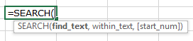  We have dummy data in column A. Column B contains the text which we will search for. And column C has the starting position of the search. And, here in column D, we will enter the SEARCH function.   1^st Example:- In the first example, we will search “AGE” in cell A7.   Follow the steps given below:-

• Enter the function in cell C7
• =SEARCH(«AGE»,A7,1)
• Press Enter

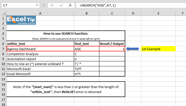  It returns to 1 because “SEARCH” is looking from the first character, and it found AGE beginning from the 1^st character. So it gives us 1 here. 2^nd Example:- In this example, we will search for “C” and we give the starting number as zero or negative number as the starting position.  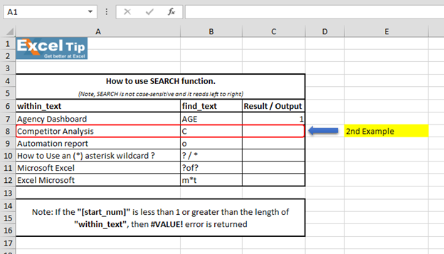 Follow the steps given below:-

• Enter the function in cell C8
• =SEARCH(«c»,A8,-1), Press Enter

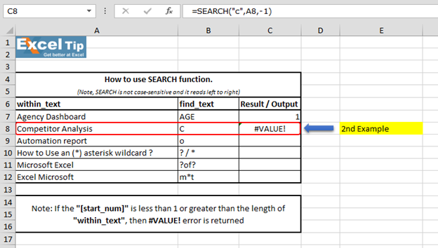  The Function has returned #VALUE error because neither negative nor 0 can be the starting position. 3^rd Example:- In this example, we will show you what if we have to find the text which is there multiple times in the string.  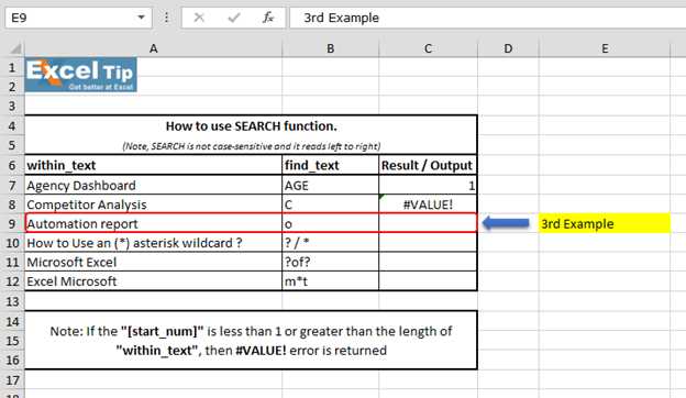 Follow the steps given below:-

• Enter the function in cell C9
• =SEARCH(«o»,A9,5), Press Enter

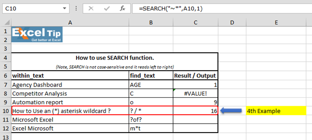
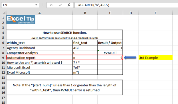  The function has ignored the “o” which is at 4^th position and the function returns to 9 as the position. Because it ignored the first “o” and started looking from 5^th character onwards. However, it returns the overall position of the string. 4^th Example:- In this example, we’ll search for wildcard characters’ position within cell A10.  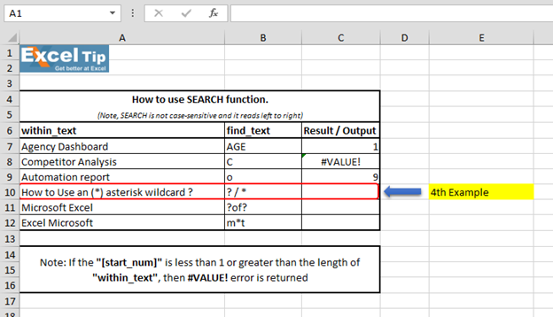 Follow the steps given below:-

• First we’ll look for (*) asterisk sign, enter the function in cell C10
• =SEARCH(«*»,A10,1), Press Enter

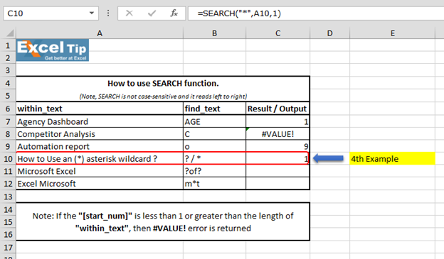  The function has returned 1, because we cannot find any wildcard without using tilde. As we use tilde (~) as a marker to indicate that the next character is a literal, we will insert (~) tilde before (*) asterisk.

• Enter this function =SEARCH(«~*»,A10,1)
• Now it returns 16 as the position

  We can also look for question mark:-

• Enter the function in same cell C10
• =SEARCH(«~?»,A10,1), Press Enter

  We can see that function gave us “37” as the position of (?) question mark. 5^th Example:- In this example, we’ll learn how to enter SEARCH function to search “?of?”.  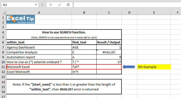 Follow the steps given below:-

• Enter the function in cell C11
• =SEARCH(«?of?»,A11,1)
• Press Enter

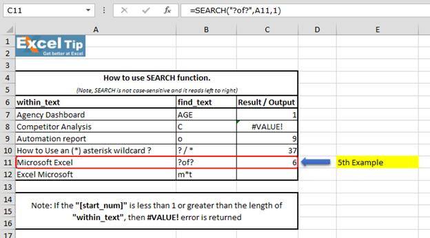  We scan to see that function has returned 6 because it matches “soft” which is present in the mid of “Microsoft Excel” string and hence the value is 6. Note:- (?) question mark wildcard denotes any single character. 6^th Example:- In this example, we’ll learn another use of wildcard in SEARCH function.   Follow the steps given below:-

• Enter the function in cell C12
• =SEARCH(«m*t»,A12,1)

Note: — In first argument, we tell the function to look for the string which starts with “m” and ends with “t”, and we will put asterisk (*) in between.

• Press Enter

  “Microsoft Excel” and it finds there is a string which starts with “M” and ends with “L”. No matter how many characters are there in between and hence it returns 1. Because (*) asterisk wild character matches any sequence of character. So, this is how SEARCH function works in different situation.  

Video: How to use SEARCH function in Microsoft Excel

Click on the video link for quick reference to the use of SEARCH function. Subscribe to our new channel and keep learning with us! https://www.youtube.com/watch?v=HW0QP1JxeuU

If you liked our blogs, share it with your friends on Facebook. And also you can follow us on Twitter and Facebook. We would love to hear from you, do let us know how we can improve, complement or innovate our work and make it better for you. Write us at info@exceltip.com