Use rank in excel

This article describes the formula syntax and usage of the RANK function in Microsoft Excel.

Description

Returns the rank of a number in a list of numbers. The rank of a number is its size relative to other values in a list. (If you were to sort the list, the rank of the number would be its position.)

Important: This function has been replaced with one or more new functions that may provide improved accuracy and whose names better reflect their usage. Although this function is still available for backward compatibility, you should consider using the new functions from now on, because this function may not be available in future versions of Excel.

For more information about the new functions, see RANK.AVG function and RANK.EQ function.

Syntax

RANK(number,ref,[order])

The RANK function syntax has the following arguments:

• Number     Required. The number whose rank you want to find.

• Ref     Required. An array of, or a reference to, a list of numbers. Nonnumeric values in ref are ignored.

• Order     Optional. A number specifying how to rank number.

  If order is 0 (zero) or omitted, Microsoft Excel ranks number as if ref were a list sorted in descending order.

  If order is any nonzero value, Microsoft Excel ranks number as if ref were a list sorted in ascending order.

Remarks

• RANK gives duplicate numbers the same rank. However, the presence of duplicate numbers affects the ranks of subsequent numbers. For example, in a list of integers sorted in ascending order, if the number 10 appears twice and has a rank of 5, then 11 would have a rank of 7 (no number would have a rank of 6).

• For some purposes one might want to use a definition of rank that takes ties into account. In the previous example, one would want a revised rank of 5.5 for the number 10. This can be done by adding the following correction factor to the value returned by RANK. This correction factor is appropriate both for the case where rank is computed in descending order (order = 0 or omitted) or ascending order (order = nonzero value).

  Correction factor for tied ranks=[COUNT(ref) + 1 – RANK(number, ref, 0) – RANK(number, ref, 1)]/2.

  In the following example, RANK(A2,A1:A5,1) equals 3. The correction factor is (5 + 1 – 2 – 3)/2 = 0.5 and the revised rank that takes ties into account is 3 + 0.5 = 3.5. If number occurs only once in ref, the correction factor will be 0, since RANK would not have to be adjusted for a tie.

Example

Copy the example data in the following table, and paste it in cell A1 of a new Excel worksheet. For formulas to show results, select them, press F2, and then press Enter. If you need to, you can adjust the column widths to see all the data.

Data
7
3.5
3.5
1
2
Formula	Description (Result)	Result
=RANK(A3,A2:A6,1)	Rank of 3.5 in the list above (3)	3
=RANK(A2,A2:A6,1)	Rank of 7 in the list above (5)	5

This tutorial demonstrates how to use the Excel RANK Function in Excel to rank a number within a series.

RANK Function Overview

The RANK Function Rank of a number within a series.

To use the RANK Excel Worksheet Function, select a cell and type:

(Notice how the formula inputs appear)

RANK function Syntax and inputs:

=RANK(number,ref,order)

number – The number that you wish to determine the rank of.

ref – An array of numbers.

order – OPTIONAL. A number indicating whether to rank descendingly (0 or Ommitted) or ascendingly (non-zero number)

What Is the RANK Function?

The Excel RANK Function tells you the rank of a particular value taken from a data range. That is, how far the value is from the top, or the bottom, when the data is put into order.

RANK Is a “Compatibility” Function

As of Excel 2010, Microsoft replaced RANK with two variations: RANK.EQ and RANK.AVG.

The older RANK Function still works, so any older spreadsheets using it will continue to function. However, you should use one of the newer functions whenever you don’t need to remain compatible with older spreadsheets.

How to Use the RANK Function

Use RANK like this:

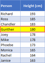
=RANK(C8,C4:C13,0)

Above is a table of data listing the heights of a group of friends. We want to know where Gunther ranks in the list.

RANK takes three arguments:

• The first is the value you want to rank (we’ve set this to C10, Gunther’s height, but we could also put the value in directly as 180)
• The second is range of data – C4:C13
• The third is the order of the rank
  • If you set this to FALSE, 0, or leave it blank, the highest value will be ranked as #1 (descending order)
  • If you set this to TRUE or any non-zero number, the lowest value will be ranked as #1 (ascending order)

RANK determines that Gunther is the 4^th tallest of the group, and if we put the data in order, we see that this is true:

A few key points about the RANK Function:

• When determining the order, text strings will result in a #VALUE! error
• As you’ve just seen, you don’t need to sort the data for RANK to work correctly

How RANK Handles Ties

In the below table I’ve added a column to the table that returns the rank of each member of the group. I used the following formula:

=RANK(C4,$C$4:$C$13,0)

Note that I’ve locked the data range $C$4:$C$13 by select “C4:C13” in the formula bar, and then pressing F4. This keeps this part of the formula the same so that you can copy it down the table without it changing.

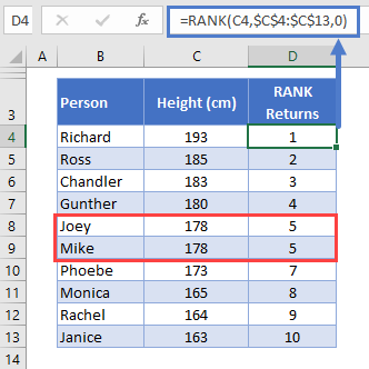
We have a tie! Both Joey and Mike are 178cm tall.

In such cases, RANK assigns both values the highest rank – so both Joey and Mike are ranked 5^th. Because of the tie, there is no 6^th place, so the next tallest friend, Phoebe, is in 7^th place.

How to Use RANK.EQ

RANK.EQ works in the same way as RANK. You use it like this:

=RANK.EQ(C10,C4:C13,0)

As you can see here, with RANK.EQ you define exactly the same arguments as with RANK, namely, the number you want to rank, the data range, and the order. We’re looking for Gunther’s rank again, and RANK.EQ returns the same result: 4.

RANK.EQ also handles ties in the same way as RANK, as shown below:

Again, Joey and Mike are tied at 5th place.

How to Use RANK.AVG

RANK.AVG is very similar to RANK.EQ and RANK. It only differs in the way it handles ties. So if you’re just looking for the rank of a single value, all three functions will return the same result:

=RANK.AVG(C6,C4:C13,TRUE)

Once again, the same result – 4^th place for Gunther.

Now let’s look at how RANK.AVG differs in terms of ties. So this time I’ve used this function:

=RANK.AVG(C5,$C$4:$C$13,0)

And here are the results:

Now we see something different!

RANK.AVG gives Joey and Mike the same rank, but this time they are assigned the average rank that they would have received had their heights not been equal.

So, they would have been ranked 5^th and 6^th, but RANK.AVG has returned the average of 5 and 6: 5.5.

If more than two values are tied, the same logic applies. Let’s pretend Phoebe has a sudden growth spurt, and her height increases to 178cm overnight. Now RANK.AVG returns the following:

All three friends how rank 6^th: (5 + 6 + 7) / 3 = 6.

RANK IF Formula

Excel doesn’t have a built-in formula that enables you to rank values based on a given criteria, but you can achieve the same result with COUNTIFS.

Say the friends want to create two separate rank orders, one for males and one for females.

Here’s the formula we’d use:

=COUNTIFS($C$4:$C$13,C4,$D$4:$D$13,">"&D4) + 1

COUNTIFS counts the number of values in a given data range that meet criteria you specify. The formula looks a little intimidating, but it makes more sense if we break it down line-by-line:

=COUNTIFS(
$C$4:$C$13,C4,
$D$4:$D$13,">"&D4
) + 1

So the first criteria we’ve set is that the range in C4:C13 (again, locked with the dollar signs so that we can drag the formula down the table without that range changing) must match the value in C4.

So for this row, we’re looking at Richard, and his value is C4 is “Male”. So we’re only going to count people who also have “Male” in this column.

The second criteria is that D4:D13 must be higher than D4. Effectively, this returns the number of people in the table who’s value in the D column is greater than Richard’s.

Then we add 1 to the result. We need to do this because no one is taller than Richard, so the formula would return 0 otherwise.

Note that this formula handles ties in the same way as RANK.EQ.

Learn more on the main page for the Excel COUNTIF Function.

RANK Function in Google Sheets

The RANK Function works exactly the same in Google Sheets as in Excel:

RANK Examples in VBA

You can also use the RANK function in VBA. Type:

application.worksheetfunction.rank(number,ref,order)

Executing the following VBA statements

Range("D2")=Application.WorksheetFunction.Rank(Range("B2"),Range("A2:A7"))
Range("D3")=Application.WorksheetFunction.Rank(Range("B3"),Range("A2:A7"))
Range("D4")=Application.WorksheetFunction.Rank(Range("B4"),Range("A2:A7"))
Range("D5")=Application.WorksheetFunction.Rank(Range("B5"),Range("A2:A7"),Range("C5"))
Range("D6")=Application.WorksheetFunction.Rank(Range("B6"),Range("A2:A7"),Range("C6"))
Range("D7")=Application.WorksheetFunction.Rank(Range("B7"),Range("A2:A7"),Range("C7"))

will produce the following results

For the function arguments (number, etc.), you can either enter them directly into the function, or define variables to use instead.

Return to the List of all Functions in Excel

Функция

РАНГ(

)

, английский вариант RANK(),

возвращает

ранг числа в списке чисел. Ранг числа — это его величина относительно других значений в списке. Например, в массиве {10;20;5} число 5 будет иметь ранг 1, т.к. это наименьшее число, число 10 — ранг 2, а 20 — ранг 3 (это ранг по возрастанию, когда наименьшему значению присваивается ранг 1). Если список отсортировать, то ранг числа будет его позицией (если нет повторов).

Синтаксис

РАНГ

(

число

;

ссылка

;порядок)

Число

— число, для которого определяется ранг.

Ссылка

— ссылка на список чисел (диапазон ячеек с числами). Напрямую массив задать нельзя, формула =РАНГ(10;{10:50:30:40:50}) работать не будет. Но, если ввести формулу

=РАНГ(B7;$A$7:$A$11)

, то она будет работать (хотя ячейка

B7

— вне списка с числами). Если в

B7

содержится число вне списка с числами, то формула вернет ошибку #Н/Д.

Нечисловые значения в ссылке игнорируются. Числам, сохраненным в текстовом формате, ранг также не присваивается, функция воспринимает их как текст.

Порядок

— число, определяющее способ упорядочения.

• Если порядок равен 0 (нулю) или опущен, то MS EXCEL присваивает ранг=1 максимальному числу, меньшим значениям присваиваются б
  
  о
  
  льшие ранги.
• Если порядок — любое ненулевое число, то то MS EXCEL присваивает ранг=1 минимальному числу, б
  
  о
  
  льшим значениям присваиваются б
  
  о
  
  льшие ранги.

Примечание

: Начиная с MS EXCEL 2010 для вычисления ранга также используются функции

РАНГ.СР()

и

РАНГ.РВ()

. Последняя функция аналогична

РАНГ()

.

Определяем ранг в списке без повторов

Если список чисел находится в диапазоне

A7:A11

, то формула

=РАНГ(A7;$A$7:$A$11)

определит ранг числа из ячейки

А7

(см.

файл примера

).

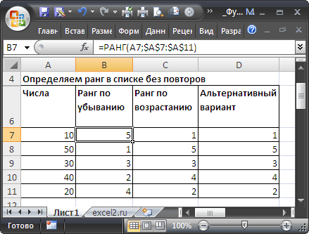
Т.к. аргумент

порядок

опущен, то MS EXCEL присвоил ранг=1 максимальному числу (50), а максимальный ранг (5 = количеству значений в списке) — минимальному (10).

Альтернативный вариант:

=СЧЁТЕСЛИ($A$7:$A$11;»>»&A7)+1

В столбце

С

приведена формула

=РАНГ(A7;$A$7:$A$11;1)

с рангом по возрастанию, ранг=1 присвоен минимальному числу. Альтернативный вариант:

=СЧЁТЕСЛИ($A$7:$A$11;»<«&A7)+1

Если исходный список

отсортировать

, то ранг числа будет его позицией в списке.

Ранг по условию

Если список состоит из значений, относящихся к разным группам (например, к разным маркам машин), то ранг можно вычислить не только относительно всей совокупности данных, но и относительно данных каждой отдельной группы.

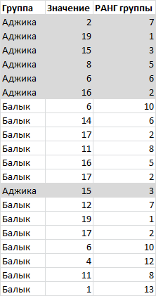
В

файле примера

ранг по условию (условием является принадлежность значения к групп) вычислен с помощью формулы:

=СЧЁТЕСЛИМН($A$3:$A$22;A3;$B$3:$B$22;»>»&B3)+1

В столбце А содержатся названия группы, в столбце В — значения.

Связь функций

НАИБОЛЬШИЙ()

/

НАИМЕНЬШИЙ()

и

РАНГ()

Функции

НАИБОЛЬШИЙ()

и

РАНГ()

являются взаимодополняющими в том смысле, что записав формулу

=НАИБОЛЬШИЙ($A$7:$A$11;РАНГ(A7;$A$7:$A$11))

мы получим тот же исходный массив

A7:A11

.

Определяем ранг в списке с повторами

Если список содержит

повторы

, то повторяющимся значениям (выделено цветом) будет присвоен одинаковый ранг (максимальный, если использована функция

РАНГ()

или

РАНГ.РВ()

) или среднее значение, если

РАНГ.СР()

). Наличие повторяющихся чисел влияет на ранги последующих чисел. Например, если в списке целых чисел, отсортированных по возрастанию, дважды встречается число 10, имеющее ранг 5, число 11 будет иметь ранг 7 (ни одно из чисел не будет иметь ранга 6).

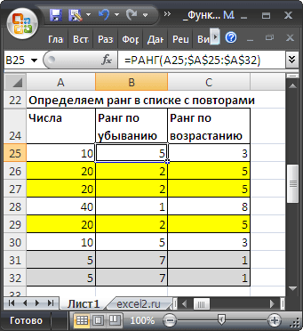
Иногда это не удобно и требуется, чтобы ранги не повторялись (например, при определении призовых мест, когда нельзя занимать нескольким людям одно место).

В этом нам поможет формула

=РАНГ(A37;A$37:A$44)+СЧЁТЕСЛИ(A$37:A37;A37)-1

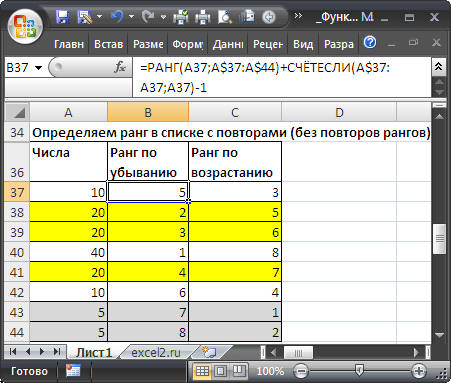
Предполагается, что исходный список с числами находится в диапазоне

А37:А44

.

Примечание

. В

MS EXCEL 2010

добавилась функция

РАНГ.РВ(число;ссылка;[порядок])

Если несколько значений имеют одинаковый ранг, возвращается наивысший ранг этого набора значений (присваивает повторяющимся числам одинаковые значения ранга). В

файле примера

дается пояснение работы этой функции. Также добавилась функция

РАНГ.СР(число;ссылка;[порядок])

Если несколько значений имеют одинаковый ранг, возвращается среднее.

Массив рангов

Для построения некоторых сложных

формул массива

может потребоваться

массив

рангов, т.е. тот же набор рангов, но в одной ячейке.

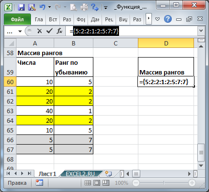
Как видно из картинки выше, значения из диапазона

В60:В67

и в ячейке

D60

совпадают. Такой массив можно получить с помощью формулы

=РАНГ(A60:A67;A60:A67)

или с помощью формулы

=СЧЁТЕСЛИ(A60:A67;»>»&A60:A67)+1

Ранги по возрастанию можно получить с помощью формулы

=РАНГ(A60:A67;A60:A67;1)

или

=СЧЁТЕСЛИ(A60:A67;»<«&A60:A67)+1

.

Такой подход использется в статьях

Отбор уникальных значений с сортировкой в MS EXCEL

и

Динамическая сортировка таблицы в MS EXCEL

.