Use or in sumifs excel - Word и Excel - помощь в работе с программами

Of all the functions introduced in Excel 2007, 2010, and 2013, my personal favorite is SUMIFS. The SUMIFS function performs multiple condition summing. The function is designed with AND logic, but, there are several techniques that allow us to use OR logic instead. This post explores a few of them.

Note: if your version of Excel has the FILTER function, check out this post as well.

Objective

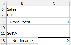
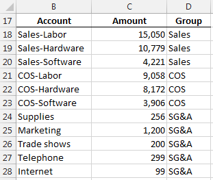
Let’s be clear about our objective by taking a look at a worksheet. Let’s assume we are trying to generate a little report based on data exported from an accounting system. We would like to write formulas to populate the report shown below.

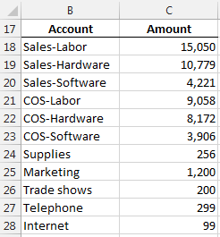
We want to populate the report by aggregating the values from the exported accounting data, shown below.

Since the SUMIFS function is designed with AND logic, the following formula wouldn’t work to populate the report’s sales value:

=SUMIFS($C$18:$C$28,
$B$18:$B$28,"Sales-Labor",
$B$18:$B$28,"Sales-Hardware",
$B$18:$B$28,"Sales-Software")

The formula wouldn’t work because there are no rows where the account is equal to Sales-Labor AND equal to Sales-Hardware AND equal to Sales-Software. As a result, the formula above returns zero.

Now that we have a clear idea of the situation, let’s work through several approaches.

SUMIFS and Wildcard

If we are lucky, there is a uniform pattern in the labels that we can use with wildcards. For example, in the data above, all of the sales accounts happen to start with “Sales-” and that makes us really lucky. We can simply use a wildcard to tell the SUMIFS function to add up any rows where the account begins with Sales- as shown in the formula below:

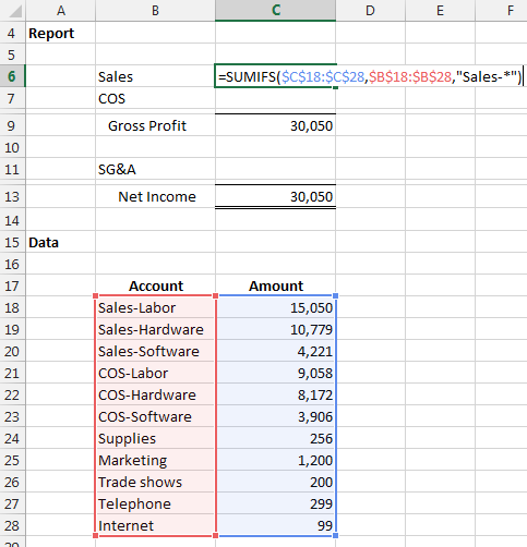
=SUMIFS($C$18:$C$28,$B$18:$B$28,"Sales-*")

Here it is in the report:

Note: Alternatively, we could reference the report label in the cell, and update the third argument to B6&”*”

A similar function could populate the COS report value, as follows:

=SUMIFS($C$18:$C$28,$B$18:$B$28,"COS-*")

And then we could populate the SG&A report value by adding up all of the accounts that do not have a dash, as follows:

=SUMIFS($C$18:$C$28,$B$18:$B$28,"<>*-*")

However, in practice, we are not often lucky enough to have such a pattern. So, let’s explore other options.

SUMIFS+SUMIFS

Another option is to simply string together a series of SUMIFS functions, each one designed to aggregate a specific label. For example, we could use SUMIFS to add up all rows where the account is equal to Sales-Labor, and then add to its result a SUMIFS function designed to add up all rows where account is equal to Sales-Hardware, and so on. This idea can be illustrated as follows:

=SUMIFS()+SUMIFS()+SUMIFS()

The corresponding formula to populate the sales report value is shown below.

=SUMIFS($C$18:$C$28,$B$18:$B$28,"Sales-Labor")+
SUMIFS($C$18:$C$28,$B$18:$B$28,"Sales-Hardware")+
SUMIFS($C$18:$C$28,$B$18:$B$28,"Sales-Software")

When there are only a couple of criteria values, this approach may get the job done. When there are several criteria values, we can simplify the formula and remove the redundancy by using an array criteria value argument. Let’s examine this approach now.

SUM(SUMIFS({}))

We can create a list of criteria values and include them in a single SUMIFS argument. To create a list like this, technically called an array, we simply surround it with {curly brackets}. There is one little trick to get this approach to work, but, let’s take it one step at a time.

First, let’s take a look at a formula that includes the account list in an array argument:

=SUMIFS($C$18:$C$28,$B$18:$B$28,{"Sales-Labor","Sales-Hardware","Sales-Software"})

You’ll notice that we used a SUMIFS function with a single criteria value argument. The criteria value argument is a comma-separated list surrounded by {curly braces}. This essentially tell’s the function to return the amounts for each of the listed accounts.

However, when we hit Enter, we notice that the formula only returns the sum of the first account, Sales-Labor. This brings us to our little trick. The array argument causes the formula to return three results, and since we wrote the formula in a single cell, we only see the first result. To have our cell show the sum of all three results, we simply enclose the SUMIFS function in a SUM function, as follows:

=SUM(SUMIFS($C$18:$C$28,
$B$18:$B$28,{"Sales-Labor","Sales-Hardware","Sales-Software"}))

Note: if you are familiar with array formulas, you can select three cells, then hit Ctrl+Enter to view the three results in three cells.

While each of the approaches above may achieve our objective, there is another approach that may work better for recurring-use workbooks. The concern with all of the options above is that they store the criteria values, the account names, in the cells as text strings. This prevents us from using consistent formulas within the report range. Whenever possible, we try to write consistent formulas within a range that can be filled down. We are unable to fill the above formulas because the criteria values are embedded in them. Since this makes the worksheet more difficult to maintain over time, it is often preferred to store the criteria values in cells and then reference the cells in the SUMIFS function. We can accomplish this by using a simple report group lookup table.

Report Group Lookup

Before we dig into the mechanics, let’s take a step back for a moment. Essentially, we are trying to group transaction values for reporting purposes, but, the group labels do not appear in the data. Had the accounting system exported the report group labels, our job would have been easy. The good news is that even though it didn’t, we can easily define the report groups with a simple lookup table.

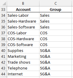
Consider the following lookup table which defines the desired report groups.

We can easily add a helper column to the data table that retrieves the proper report group. We can use our favorite lookup function to accomplish this task. For example, the following formula retrieves the report group with a VLOOKUP function:

=VLOOKUP(B18,$B$34:$C$44,2,0)

When we fill the formula down, the updated data table includes the report group, as shown below.

Now, we can populate the report’s sales value with a simple formula.

=SUMIFS($C$18:$C$28,$D$18:$D$28,B6)

We can fill this formula down throughout the report as shown below.

The consistent formulas make us very happy and the report group column makes it clear how the values flow into the report.

If you have any other techniques for using OR logic with SUMIFS, please share by posting a comment below…thanks!

Additional Resources

Download sample file: SUMIFS with OR
The SUMPRODUCT function can also be used to perform conditional summing with OR logic
If you needed to use OR logic for numerous column, instead of within a single column as discussed above, be careful not to double-count rows that meet both criteria
Excel University Volume 2 explores the SUMIFS and VLOOKUP functions in detail

Источник

17 авг. 2022 г.
читать 2 мин

Вы можете использовать следующие формулы для объединения функции СУММЕСЛИ с функцией ИЛИ в Excel:

Метод 1: СУММЕСЛИ с ИЛИ (один столбец)

=SUM(SUMIFS( B2:B13 , A2:A13 ,{"Value1","Value2", "Value3"}))

Эта конкретная формула находит сумму значений в B2:B13 , где соответствующее значение в A2:A13 содержит «Value1», «Value2» или «Value3».

Метод 2: СУММЕСЛИ с ИЛИ (несколько столбцов)

=SUMIF( A2:A13 ,"Value1", C2:C13 )+SUMIF( B2:B13 ,"Value2", C2:C13 )

Эта конкретная формула находит сумму значений в C2:C13 , где соответствующее значение в A2:A13 содержит «Value1» или соответствующее значение в B2:B13 содержит «Value2».

В следующем примере показано, как использовать каждый метод на практике со следующим набором данных в Excel:

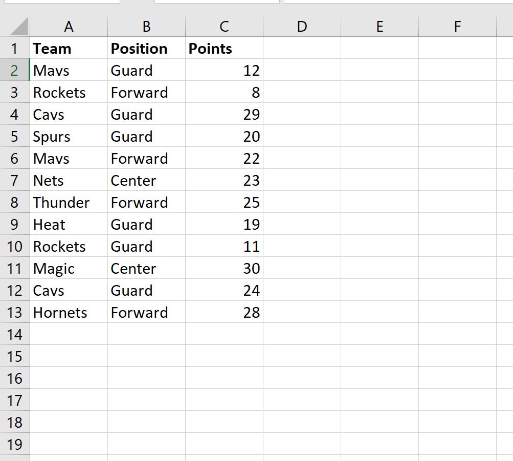
Пример 1: СУММЕСЛИ с ИЛИ (один столбец)

Мы можем использовать следующую формулу для суммирования значений в столбце Points , где значение в столбце Team равно «Mavs» или «Rockets»:

=SUM(SUMIFS( C2:C13 , A2:A13 ,{"Mavs","Rockets"}))

На следующем снимке экрана показано, как использовать эту формулу на практике:

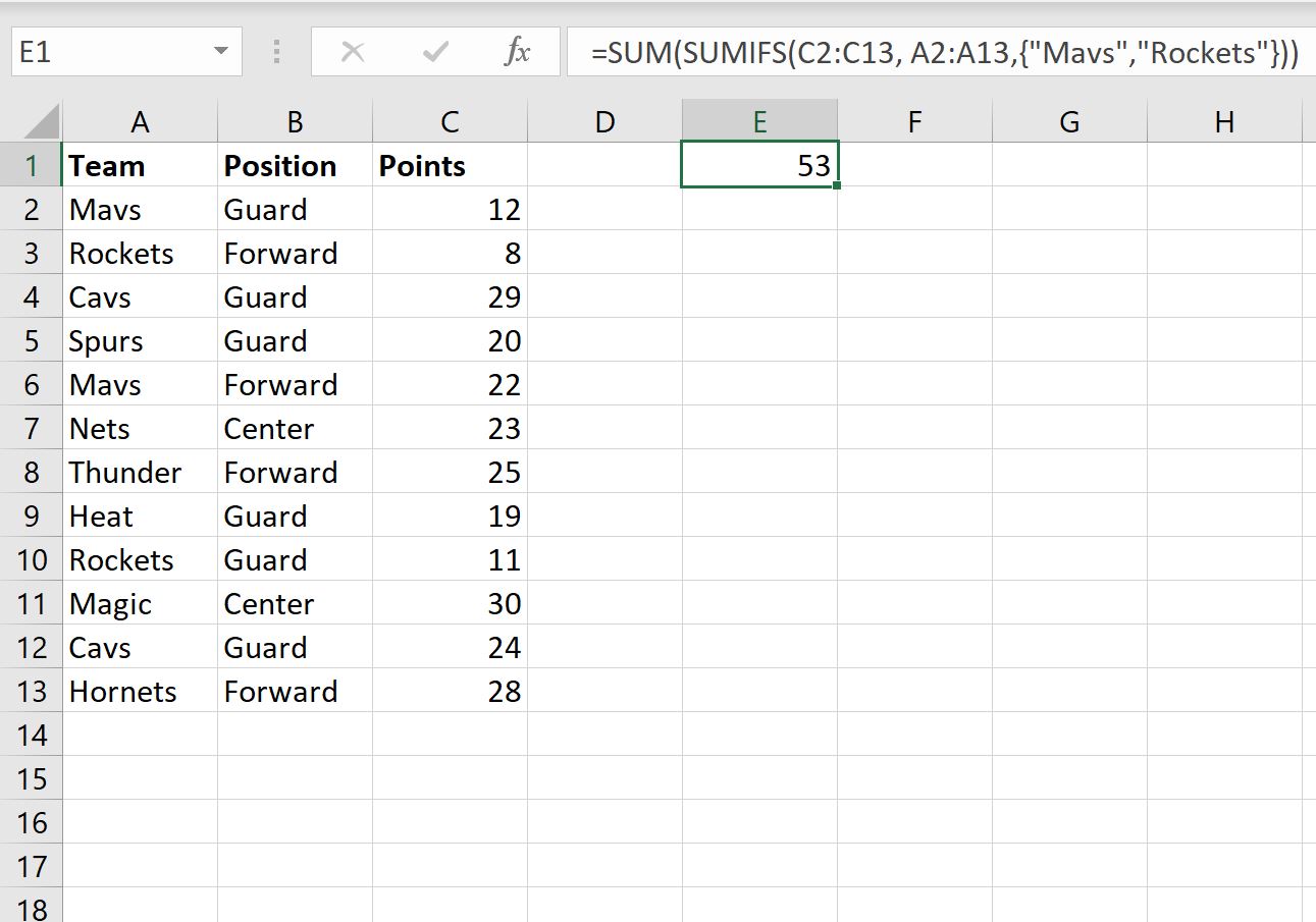
Сумма значений в столбце « Очки », где значение в столбце « Команда » равно «Mavs» или «Rockets», составляет 53 .

Пример 2: СУММЕСЛИ с ИЛИ (несколько столбцов)

Мы можем использовать следующую формулу для суммирования значений в столбце Points , где значение в столбце Team равно «Mavs» или значение в столбце Position равно «Center»:

=SUMIF( A2:A13 ,"Mavs", C2:C13 )+SUMIF( B2:B13 ,"Center", C2:C13 )

На следующем снимке экрана показано, как использовать эту формулу на практике:

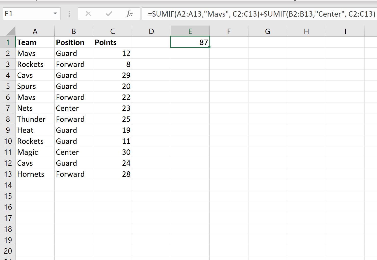
Сумма значений в столбце « Очки », где значение в столбце « Команда » равно «Mavs» или значение в столбце « Позиция » равно «Центру», составляет 87 .

Дополнительные ресурсы

В следующих руководствах объясняется, как выполнять другие распространенные операции СУММЕСЛИ в Excel:

Как использовать СУММЕСЛИМН с диапазоном дат в Excel
Как суммировать, если ячейки содержат текст в Excel

Источник

Sometimes we need to make small amendments to formulas to make them effective.

Just like that, SUMIF OR. It’s an advanced formula that helps you to increase the flexibility of SUMIF. Yes, you can also do SUMIFS as well. But before we use it let me tell you one thing about SUMIF.

In SUMIF, you can only use one criterion and in SUMIFS, you can use more than one criterion to get a sum.

Just a thing like this. Let’s say, in SUMIFS, if you specify two different criteria, it will sum only those cells which meet both of the criteria.

Because it works with AND logic, all the criteria should meet to get a cell included. When you combine OR logic with SUMIF/SUMIFS you can sum values using two different criteria at the same time.

Without any further ado let’s learn this amazing formula.

Do We Really Need OR Logic? Any Example?

Let me show you an example where we need to add an OR logic in SUMIFS or SUMIF.

Take a look at below data table where you have a list of products with their quantity and the current status of the shipment.

data table to use or logic to use in sumifs sumif

In this data, you have two types of products (Faulty and Damaged) that you need to return to our vendor.

But before that, you want to calculate the total quantity of both types of products. If you go with the normal method, you have to apply SUMIF twice to get this total.

But if you use an OR condition in SUMIF then you can get the total of both of the products with just one formula.

OK, Let’s Apply OR with SUMIFS

Before we start, please download this sample file from here to follow along.

In any other cell in your worksheet where you want to calculate the total, insert the below formula and hit enter.

=SUM(SUMIFS(C2:C21,B2:B21,{"Damage","Faulty"}))

In the above formula, you have used SUMIFS but if you want to use SUMIF you can insert the below formula in the cell.

=SUM(SUMIF(B2:B21,{"Damage","Faulty"},C2:C21))

By using both of the above formulas you will get 540 in the result. To cross-verify, just check the total manually.

verify the total of damage and faulty using sumif or

How this formula Works

As I said, the SUMIFS function uses AND logic to sum values. But, the formula which you have used above includes an OR logic in it.

To understand this formula you have to split it into three different parts.

three parts of formula to use or logic in sumifs sumif

The first thing is to understand that, you have used two different criteria in this formula by using the array concept. Learn more about the array from here.
The second thing is when you specify two different values using an array, SUMIFS has to look for both of the values separately.
The third thing is even after using an array formula, SUMIFS is not able to return the sum of both of the values in a single cell. So, that’s why you have to enclose it with the SUM function.

With the above concept, you are able to get a total for both types of products in a single cell.

It will work the same with SUMIF and SUMIFS.

And, you can also further expand your formula by specifying the product name in the second criteria in SUMIFS to get the total for a single product.

sample-file

Using Dynamic Criteria Range

In the comment section, Shay asked me about using a cell reference to add multiple criteria instead of inserting them directly into the formula.

Well, that’s a super valid question and you can do this by using a dynamic named range instead of hardcore values.

And for this, you need to do just two little amendments to your formula.

The first is that instead of using curly brackets you need to use a named range (the best way is to use a table) of your value.
And after that, you need to enter this formula by using Ctrl + Shift + Enter as a proper array formula.

So, now your formula will be:

Let me take you to next level of this formula. Just look at the below data table.

sumifs sumif or with multiple column data

In this table, you have two different columns with two different kinds of statuses. Now, from this data table, you need to sum the quantity where the product is damaged return status is “No”.

That means only those Damage and Faulty products which are not been returned yet. And, the formula for this will be.

=SUM(SUMIFS(D2:D21,B2:B21,{"Damage","Faulty"},C2:C21,"No"))

sumifs sumif or with multiple different column criteria formula

sample-file

Conclusion

The best part about using the OR technique is you can add as many criteria to it. If you want to use only OR logic then it’s fine to use SUMIF. And if you want to create an OR condition and AND condition in a single formula then you can use SUMIFS for that.

You know, this is one of my favorite formula tips and I hope you found it useful.

Now tell me one thing. Have you ever used this kind of formula before? Share your views with me in the comment section, I’d love to hear from you, and please don’t forget to share this tip with your friends.

Источник

In this article, we will learn how to use AND — OR logic in SUMIFS function in Excel.

AND logic is used when all conditions stated need to be satisfied.
OR logic is used when any condition stated satisfies.

In simple words, Excel lets you perform these both logic in SUMIFS function.

SUMIFS with Or

OR logic with SUMIFS is used when we need to find the sum if value1 or value2 condition satisfy
Syntax of SUMIFS with OR logic

=SUM(SUMIFS ( sum_range, criteria_range, { «value1«, «value2» }))

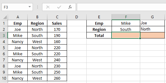
Here we need to find the sum of Sales range If “Mike” or “Joe” occurs in Emp range
Use

=SUM(SUMIFS(C2:C10,A2:A10,{«Mike»,»Joe»}))

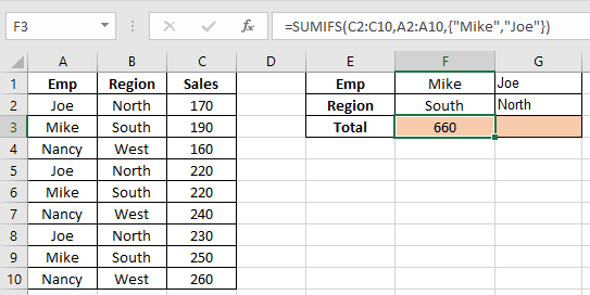
As you can see we got the sum of combined Joe’s and Mike’s sales.

SUMIFS with AND

AND logic with SUMIFS function is used when we need to find the sum if value1 and value2 both condition satisfy
Syntax of SUMIFS with AND logic

=SUMIFS ( sum_range, criteria_range1, value1, [criteria_range2, value2],.. )

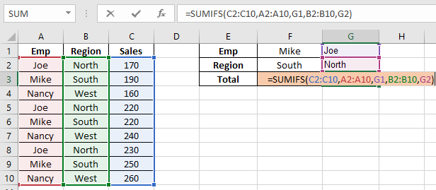
Here we need to find the sum of Sales range If “Joe” occurs in Emp range and “North” occurs in the Region range
Use

=SUMIFS ( C2:C10, A2:A10, G1, B2:B10, G2)

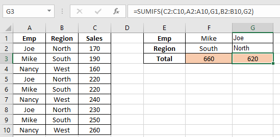
As you can see we got the sum of just Joe’ North region.

Hope you understood how to use SUMIFS function with AND-OR logic in Excel. Explore more Mathematical functions with logic_test articles on Excel TEXT function here. Please feel free to state your query or feedback for the above article.

Related Articles:

3 SUMIF examples with Or Formula in Excel

How to Use SUMIF Function in Excel

How to Use SUMIFS Function in Excel

How to Sum if cells contain specific text in Excel

How to Sum If Greater Than 0 in Excel

SUMIFS with dates in Excel

Popular Articles:

50 Excel Shortcuts to Increase Your Productivity

How to use the VLOOKUP Function in Excel

How to use the COUNTIF function in Excel

How to use the SUMIF Function in Excel

Источник

In this example, the goal is to sum the value of orders that have a status of «Complete» or «Pending». This is a slightly tricky problem in Excel because the SUMIFS function is designed for conditional sums based on multiple criteria, but all criteria must be TRUE in order for a value to be included in the sum. In other words, criteria used in the SUMIFS function is joined with AND logic, not OR logic. In simple scenarios, a simple solution is to use the SUMIFS function with an array constant.

SUMIFS function

The SUMIFS function sums the values in a range that meet multiple criteria. It is similar to the SUMIF function, which only allows a single condition, but SUMIFS allows multiple criteria, using AND logic. This can be illustrated with the following formulas:

=SUMIFS(E5:E16,D5:D16,"complete") // returns 150
=SUMIFS(E5:E16,D5:D16,"pending") // returns 50
=SUMIFS(E5:E16,D5:D16,"complete",D5:D16,"pending") // returns 0

Notice the first two formulas correctly return the total of complete and pending orders, but the last formula returns zero because an order cannot be «Complete» and «Pending» at the same time. This is because the SUMIFS function only allows AND logic – all conditions must be TRUE in order for a value to be included in the sum.

SUMIFS + SUMIFS

One simple solution is to use SUMIFS twice in a formula like this:

=SUMIFS(E5:E16,D5:D16,"complete")+SUMIFS(E5:E16,D5:D16,"pending")

This formula returns a correct result of $200, but it is redundant and doesn’t scale well.

SUMIFS + array constant

Another option is to supply SUMIFS with an array constant that holds more than one criteria like this:

=SUMIFS(E5:E16,D5:D16,{"complete","pending"}) // returns {150,50}

Through a formula behavior called «lifting», this will cause SUMIFS to be evaluated twice, once for «complete» and once for «pending», and SUMIFS will return two results in an array like this:

{150,50}

If you enter the formula above in the latest version of Excel, which supports dynamic array formulas, you will see both results spill into a range that contains two cells. Because we want a single result, we nest the SUMIFS function in the SUM function like this:

=SUM(SUMIFS(E5:E16,D5:D16,{"complete","pending"}))

This is the formula used in the worksheet shown. The formula evaluates like this:

=SUM(SUMIFS(E5:E16,D5:D16,{"complete","pending"}))
=SUM({150,50})
=200

With wildcards

You can use wildcards in the criteria if needed. For example, to sum items that contain «red» or «blue» anywhere in the criteria_range, you can use:

=SUM(SUMIFS(sum_range,criteria_range,{"*red*","*blue*"}))

Adding another OR criteria

You can add one more OR-type criteria to this formula, but you’ll need to use a horizontal array for one criteria and a vertical array for the other. So, for example, to sum orders that are «Complete» or «Pending», when the customer is «Andy Garcia» or «Bob Jones», you can use a formula like this:

=SUM(SUMIFS(E4:E16,D4:D16,{"complete","pending"},C4:C16,{"Bob Jones";"Andy Garcia"}))

Note the semi-colons in the second array constant, which represents a vertical array. This works because Excel «pairs» elements in the two array constants, and returns a two dimensional array of results. To apply additional criteria, you will want to move to a formula based on SUMPRODUCT.

Cell references for criteria

You can’t use cell references inside an array constant, you must use a proper range. When you switch from array constants to ranges, the formula becomes an array formula in older versions of Excel and must be entered with control + shift + enter:

={SUM(SUMIFS(range1,range2,range3))}

Where range1 is the sum range, range2 is the criteria range, and range3 contains multiple criteria on the worksheet. With two OR criteria, you’ll need to use horizontal and vertical arrays as explained above.

Note: this is an array formula and must be entered with control + shift + enter.

Источник

The SUMIF function in Excel is used to sum values based on a single condition or criteria. However, if we want to sum values based on multiple criteria where at least one of the conditions are met, we use the SUMIF with OR logic. There are different methods to do this.

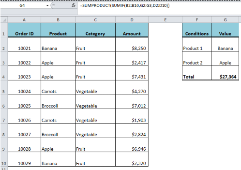
Figure 1. Final result

Adding Multiple SUMIF Functions

We sum the results of multiple SUMIF functions in one cell where each SUMIF function handles one condition or criteria. In our dataset, we have a table of products’ orders and their values. We need to add up the orders’ values of two products “Banana” and “Apple”, whichever is available using SUMIF with OR criteria in the following formula;

=SUMIF(B2:B10,"Banana",D2:D10)+SUMIF(B2:B10,"Apple",D2:D10)

=SUMIF(B2:B10,G2,D2:D10)+SUMIF(B2:B10,G3,D2:D10)

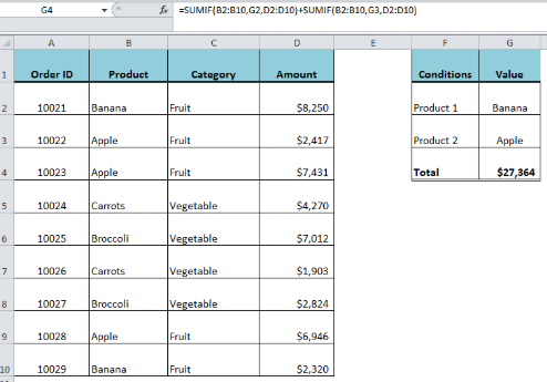Figure 2. Adding multiple SUMIF functions

Using SUM and SUMIF with an Array Constant

Here, we supply more than one value of the criteria using an array constant in criteria argument of the SUMIF function. An Array constant is a list of criteria values, separated by commas, and this list of values is enclosed in curly brackets. As we have more than one value as criteria in the array constant, so the SUMIF function will return one result for each value of criteria in the array. Therefore, we finally wrap the SUMIF function in the SUM function to add up the results of each criterion based on the SUMIF with OR criteria.

=SUM(SUMIF(B2:B10,{"Banana","Apple"},D2:D10))

Note that the criteria values in the array constant are supplied directly and not as a cell reference. The text values are supplied in double quotation marks, and numeric values are supplied without double quotation marks.

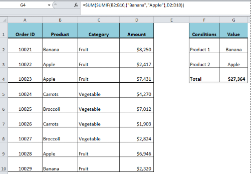Figure 3. Using SUM and SUMIF function with an array constant

Using SUMIF with SUMPRODUCT Function

If we want to list the criteria values in cell references rather than supplying them directly in the formula, we wrap the SUMIF function in the SUMPRODUCT function. The criteria values are listed in the range of cells and then we supply this range in the criteria argument of the SUMIF function. The SUMIF function returns the result for each criteria value as an array of values and the SUMPRODUCT returns the sum of those resulting values based on the SUMIF with OR criteria. In this example, the values of the products are listed in range G2:G3 as criteria argument in the SUMIF function in the following formula.

=SUMPRODUCT(SUMIF(B2:B10,G2:G3,D2:D10))

Figure 4. Using SUMIF with SUMPRODUCT function

Instant Connection to an Expert through our Excelchat Service:

Most of the time, the problem you will need to solve will be more complex than a simple application of a formula or function. If you want to save hours of research and frustration, try our live Excelchat service! Our Excel Experts are available 24/7 to answer any Excel question you may have. We guarantee a connection within 30 seconds and a customized solution within 20 minutes.

Источник

SUMIF with OR (Table of Contents)

SUMIF with OR in Excel
How to Use SUMIF with OR in Excel?

SUMIF with OR Function in Excel

SUMIF is one of the functions which is very much useful to find the totals of similar values. It reduces the time when we are working with a large amount of data and need to calculate the sum of values of similar nature data. SUMIF is a combination of SUM and IF functions. SUMIF function will perform SUM(addition) when the IF condition satisfies. It is very easy to apply.

Syntax of the SUMIF function

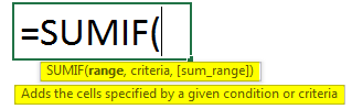
Range – A range of cells on which the criteria or condition is to be applied. The range can include a number, cell references, and names as well.
Criteria – It is the condition in the form of number, expression, or text that defines which cells will be added.
Sum_range – These are actual cells to sum. If omitted, cells specified in a range are used.

How to Use SUMIF with OR Criteria in Excel?

Let’s understand how to use SUMIF with OR Function in Excel using some examples.

You can download this SUMIF with OR Excel Template here – SUMIF with OR Excel Template

SUMIF with OR – Example #1

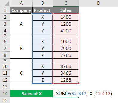
Consider a table having the sales data of companies A, B, and C for products X, Y, and Z.

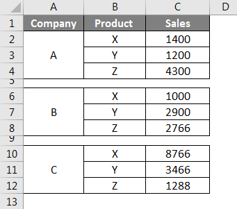
In the above screenshot, we can observe the sales of products X, Y, and Z. Now, we need to calculate the sum of sales of X in all three companies A, B, and C.

First, select a cell where we want the results of the sum of ‘X’ sales, then apply the function and select the range.

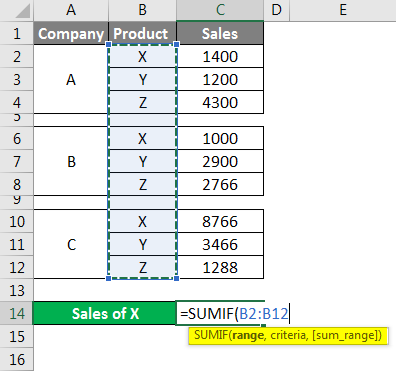
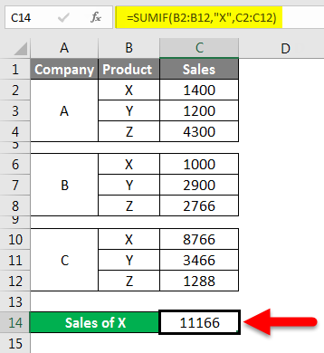
Here the range is from B2 to B12, so select that range then the function will automatically pick B2:B12 as shown in the above screenshot. Once the range is picked, give the comma as per syntax. Later give the “Criteria” here. Criteria are “X” as we want to find the SUM of X product sales, so give X and again comma.

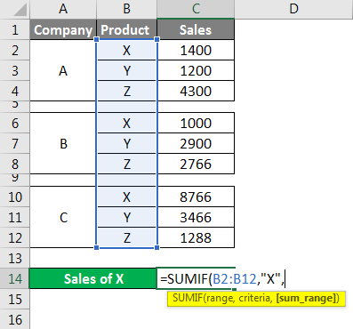
Last, we need to select the sum_range; here, sales is the range which we need to add whenever the product is X; hence select the sales range from C2:C12 as shown in the below screenshot.

The sum of sales of X across all the three companies is 11166.

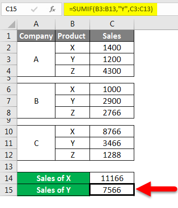
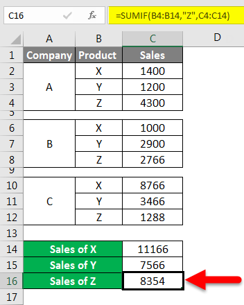
Similarly, we can find the sales of Y and Z also.

Make sure you are using the commas and a double column for criteria; otherwise, the formula will throw an error. Normally SUMIF will work on the logic, AND hence that is the reason where ever the criteria match, it will perform the addition and return the results.

By using normal SUMIF, we will be able to perform SUM operation for only single criteria. If we are using OR logic, then we can perform SUM calculation for dual criteria.

For using OR logic, we should use SUMIFS instead of SUMIF because SUMIF can perform with single criteria, but SUMIFS can perform on multiple criteria as per our requirement.

SUMIF with OR – Example #2

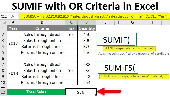
We will now consider a small table with data of sales and revenue through online and direct as below.

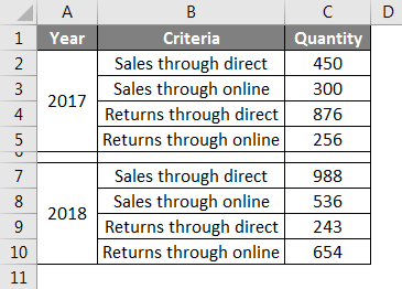
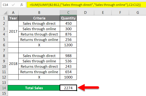
Our task is calculating the total value of sales, whether it is through direct or online. Now we will apply the SUMIFS formula to find the total sales.

It is a bit different from the SUMIF as in this first; we will select the sum range. Here sum range means the column where the values are available to perform addition or sum.

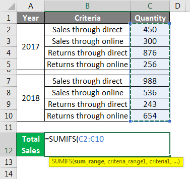
Observe the above screenshot the quantity is the column we need to add; hence select the cells from C2 to C10 as sum_range. The next step is the selection of criteria_range1.

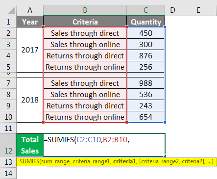
Here Criteria is “Sales through direct” and “Sales through online”; hence we need to select the column B data from B2 to B10.

Later we need to give the Criteria1 and then criteria _range2, criteria 2, but here we will do a small change. We will give criteria1 and criteria2 in a curly bracket like an array.

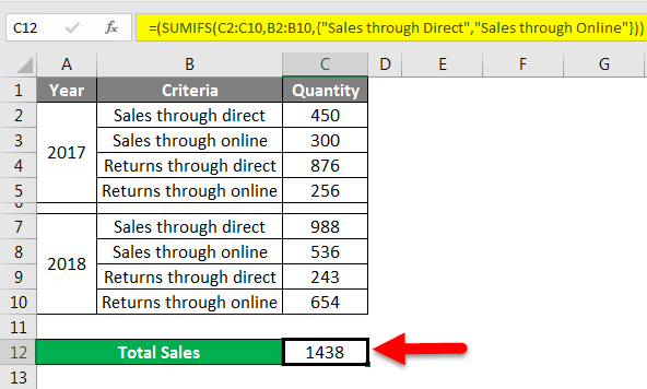
See, we got the result as 1438; let’s check whether it picked the total correctly or not. Apply a filter and filter only sales through direct and sales through online and select the entire quantity and observe the total at the bottom of the screen. Observe the below screenshot; I have highlighted the count and sum of the values.

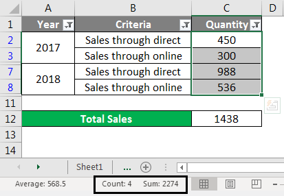
So, the total should be 2274, but we got the result of 1438. Then how this 1438 comes and what sum is this.

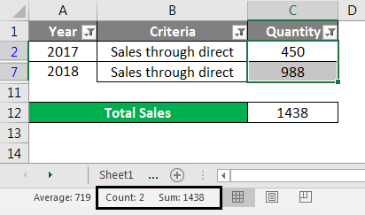
Observe the above screenshot that 1438 is the total sales for sales through direct. The formula did not pick the sales through online because we gave the formula in a different format that is like an array. Hence, if we add one more SUM formula to SUMIFS, it will perform both criteria.

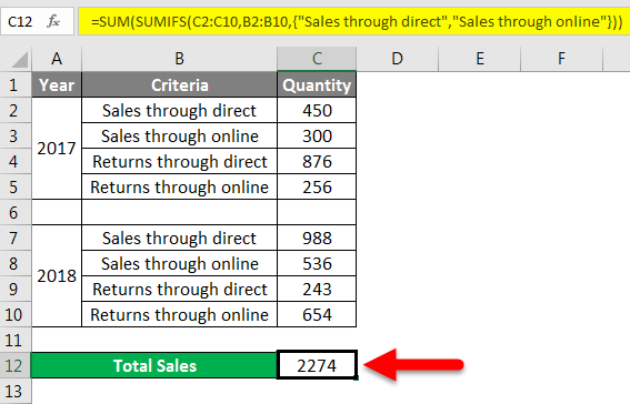
Observe the formula in the above screenshot one more SUM added to the SUMIF, and the result is 2274.

I will explain why we used another SUM function and how it works. When we gave SUMIFS function with two criteria as in the form of an array, it will calculate the sum of sales through directly and online separately. To get the sum of both, we have used another SUM function which will add the sum of two sales. If we want to add one more criteria, we can add it in the same formula.

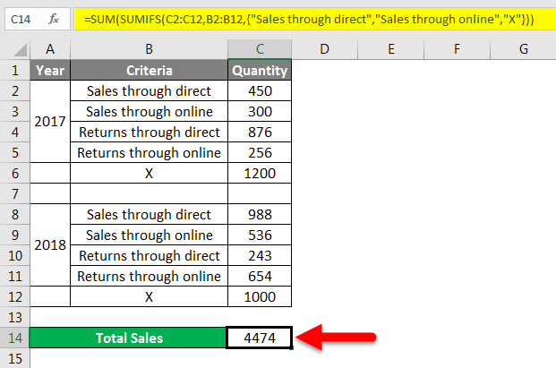
Observe the formula; we added the criteria X in the curly brackets of an array, adding the quantity X to the existing sum quantity.

In case if you want to use only SUMIF and do not want to use SUMIFS, then apply the formula in below way.

Observe the formula in the above screenshot. In this case, first, we gave the criteria range and then criteria1 and criteria2 and the last sum_range.

If we want to perform a sum based on two columns of data, consider the same data we used up to now. We need to add one more column, which is called “Tax”, as below. There is a comment ‘yes’ under the TAX column.

Now the task is to calculate the sum of quantity for the sales through direct and sales through online, which has “Yes” under the tax column.

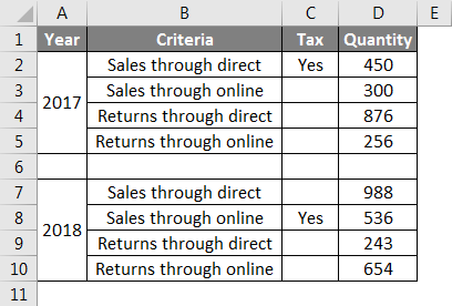
Apply the formula as shown in the below screenshot to get the sum of sales which has “Yes” under the Tax column.

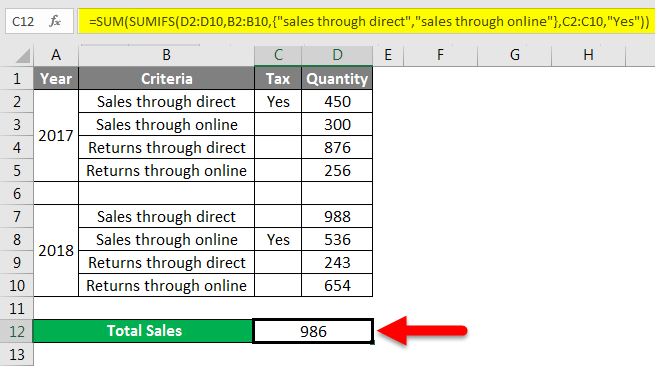
After the normal SUMIFS formula, just adds another criteria range: tax column range C2 to C10, and give criteria “Yes” in double-quotes.

Now the formula will check for criteria 1 with yes and criteria 2 with yes and add both.

Things to Remember About SUMIF with OR

SUMIF follows the AND logic that means it will perform an addition operation when if the criteria match.
SUMIFS will follow the OR and logic; that is why we can perform multiple criteria at a time.

SUMIFS with OR

Note: if your version of Excel has the FILTER function, check out this post as well.

Objective

We want to populate the report by aggregating the values from the exported accounting data, shown below.

Since the SUMIFS function is designed with AND logic, the following formula wouldn’t work to populate the report’s sales value:

The formula wouldn’t work because there are no rows where the account is equal to Sales-Labor AND equal to Sales-Hardware AND equal to Sales-Software. As a result, the formula above returns zero.

Now that we have a clear idea of the situation, let’s work through several approaches.

SUMIFS and Wildcard

Here it is in the report:

Note: Alternatively, we could reference the report label in the cell, and update the third argument to B6&”*”

A similar function could populate the COS report value, as follows:

And then we could populate the SG&A report value by adding up all of the accounts that do not have a dash, as follows:

However, in practice, we are not often lucky enough to have such a pattern. So, let’s explore other options.

SUMIFS+SUMIFS

The corresponding formula to populate the sales report value is shown below.

SUM(SUMIFS(<>))

We can create a list of criteria values and include them in a single SUMIFS argument. To create a list like this, technically called an array, we simply surround it with . There is one little trick to get this approach to work, but, let’s take it one step at a time.

First, let’s take a look at a formula that includes the account list in an array argument:

You’ll notice that we used a SUMIFS function with a single criteria value argument. The criteria value argument is a comma-separated list surrounded by . This essentially tell’s the function to return the amounts for each of the listed accounts.

Note: if you are familiar with array formulas, you can select three cells, then hit Ctrl+Enter to view the three results in three cells.

Report Group Lookup

Consider the following lookup table which defines the desired report groups.

When we fill the formula down, the updated data table includes the report group, as shown below.

Now, we can populate the report’s sales value with a simple formula.

We can fill this formula down throughout the report as shown below.

The consistent formulas make us very happy and the report group column makes it clear how the values flow into the report.

If you have any other techniques for using OR logic with SUMIFS, please share by posting a comment below…thanks!

Источник

Excel SUMIF with OR

SUMIF with OR (Table of Contents)

SUMIF with OR Function in Excel

Excel functions, formula, charts, formatting creating excel dashboard & others

Syntax of the SUMIF function

Range – A range of cells on which the criteria or condition is to be applied. The range can include a number, cell references, and names as well.
Criteria – It is the condition in the form of number, expression, or text that defines which cells will be added.
Sum_range – These are actual cells to sum. If omitted, cells specified in a range are used.