Use of or statement in if statement in excel

IF function is undoubtedly one of the most important functions in excel. In general, IF statements give the desired intelligence to a program so that it can make decisions based on given criteria and, most importantly, decide the program flow.

In Microsoft Excel terminology, IF statements are also called «Excel IF-Then statements». IF function evaluates a boolean/logical expression and returns one value if the expression evaluates to ‘TRUE’ and another value if the expression evaluates to ‘FALSE’.

Definition of Excel IF Function

According to Microsoft Excel, IF function is defined as a formula which «checks whether a condition is met, returns one value if true and another value if false».

Syntax

Syntax of IF function in Excel is as follows:

=IF(logic_test, [value_if_true], [value_if_false])

'logic_test' (required argument) – Refers to the boolean expression or logical expression that needs to be evaluated.
'value_if_true' (optional argument) – Refers to the value that will be returned by the IF function if the 'logic_test' evaluates to TRUE.
'value_if_false' (optional argument) – Refers to the value that will be returned by the IF function if the 'logic_test' evaluates to FALSE.

Important Characteristics of IF Function in Excel

• To use the IF function, you need to provide the 'logic_test' or conditional statement mandatorily.
• The arguments 'value_if_true'and 'value_if_false' are optional, but you need to provide at least one of them.
• The result of the IF statement can only be any one of the two given values (either it will be 'value_if_true' or 'value_if_false'). Both values cannot be returned at the same time.
• IF function throws a ‘#Name?’ error if the'logic_test' or boolean expression you are trying to evaluate is invalid.
•  Nesting of IF statements is possible, but Excel only allows this to 64 levels. Nesting of IF statement means using one if statement within another.

Comparison Operators That Can Be Used With IF Statements

Following comparison operators can be used within the 'logic_test' argument of the IF function:

• = (equal to)
• <> (not equal to)
• < (less than)
• > (greater than)
• >= (greater than or equal to)
• <= (less than or equal to)
• Apart from these, you can also use any other function that returns a boolean result (either ‘true’ or ‘false’). For example – ISBLANK, ISERROR, ISEVEN, ISODD, etc

Now, let’s see some simple examples to use these comparison operators within the IF Function:

Simple Examples of Excel IF Statement

Now, let’s try to see a simple example of the Excel IF function:

Example 1: Using ‘equal to’ comparison operator within the IF function

In this example, we have a list of colors, and we aim to find the ‘Blue’ color. If we are able to find the ‘Blue’ color, then in the adjacent cell, we need to assign a ‘Yes’; otherwise, assign a ‘No’.

So, the formula would be:

=IF(A2="Blue", "No", "Yes")

This suggests that if the value present in cell A2 is ‘Blue’, then return a ‘Yes’; otherwise, return a ‘No’.

If we drag this formula down to all the rows, we will find that it returns ‘Yes’ for the cells with the value ‘Blue’ for all others; it would result in ‘No’.

Example 2: Using ‘not equal to’ comparison operator within the IF function.

Let’s take example 1, and understand how we can reverse the logic and use a ‘not equal to’ operator to construct the formula so that it still results in ‘Yes’ for ‘Blue’ color and ‘No’ for any other text.

So the formula would be:

=IF(A2<>"Blue", "No", "Yes")

This suggests that if the value at A2 is not equal to ‘Blue’, then return a ‘No’; otherwise, return a ‘Yes’.

When dragged down to all the below rows, this formula would find all the cells (from A2 to A8) where the value is not ‘Blue’ and marks a ‘No’ against them. Otherwise, it marks a ‘Yes’ in the adjacent cells.

Example 3: Using ‘less than’ operator within the IF function.

In this example, we have scores of some students, along with their names. We want to assign either «Pass» or «Fail» against each student in the result column.

Based on our criteria, the passing score is 50 or more.

For this, we can use the IF function as:

=IF(B2<50,"Fail","Pass")

This suggests that if the value at B2, i.e., 37, is less than 50, then return «Fail»; otherwise, return «Pass».

As 37 is less than 50 so the result will be «Fail».

We can drag the above-given formula for the rest of the cells below and the result would be correct.

Example 4: Using ‘greater than or equal to’ operator within the IF statement.

Let’s take example 3 and see how we can reverse the logic and use a ‘greater than or equal to’ operator to construct the formula so that it still results in ‘Pass’ for scores of 50 or more and ‘Fail’ for all the other scores.

For this, we can use the Excel IF function as:

=IF(B2>=50,"Pass","Fail")

This suggests that if the value at B2, i.e., 37 is greater than or equal to 50, then return «Pass»; otherwise, return «Fail».

As 37 not greater than or equal to 50 so the result will be «Fail».

When dragged down for the rest of the cells below, this formula would assign the correct result in the adjacent rows.

Example 5: Using ‘greater than’ operator within the IF statement.

In this example, we have a small online store that gives a discount to its customers based on the amount they spend. If a customer spends $50 or more, he is applicable for a 5% discount; otherwise, no discounts are offered.

To find whether a discount is offered or not, we can use the following excel formula:

=IF(B2>50,"5% Discount","No Discount")

This translates to – If the value at B2 cell is greater than 50, assign a text «5% Discount» otherwise, assign a text «No Discount» against the customer.

In the first case, as 23 is not greater than 50, the output will be «No Discount».

We can drag the above-given formula for the rest of the cells below are the result would be correct.

Example 6: Using ‘less than or equal to’ operator within the IF statement.

Let’s take example 5 and see how we can reverse the logic and use a ‘less than or equal to’ operator to construct the formula so that it still results in a ‘5% Discount’ for all customers whose total spend exceeds $50 and ‘No Discount’ for all the other customers.

For this, we can use the IF-then statement as:

=IF(B2<=50,"No Discount","5% Discount")

This means that if the value at B2, i.e., 23, is less than or equal to 50, then return «No Discount»; otherwise, return «5% Discount».

As 23 is less than or equal to 50 so the result will be «No Discount».

When dragged down for the rest of the cells below, this formula would assign the correct result in the adjacent rows.

Example 7: Using an Excel Logical Function within the IF formula in Excel.

In this example, let’s suppose we have a list of numbers, and we have to mark Even and Odd numbers. We can do this using the IF condition and the ISEVEN or ISODD inbuilt functions provided by Microsoft Excel.

ISEVEN function returns ‘true’ if the number passed to it is even; otherwise, it returns a ‘false’. Similarly, ISODD function return ‘true’ if the number passed to it is odd; otherwise, it returns a ‘false’.

For this, we can use the IF-then statement as:

=IF(ISEVEN(A2),"Even","Odd")

This means that – If the value at A2 cell is an even number, then the result would be «Even»; otherwise, the result would be «Odd».

Alternatively, the above logic can also be written using the ISODD function along with the IF statement as:

=IF(ISODD(A2),"Odd","Even")

This means that – If the value at A2 cell is an odd number, then the result would be «Odd»; otherwise, the result would be «Even».

Example 8: Using the Excel IF function to return another formula a result.

In this example, we have Employee Data from a company. The company comes up with a simple way to reward its loyal employees. They decide to give the employees an annual bonus based on the years spent by the employee within the organization.

Employees with experience of more than 5 years are given 10% of annual salary as a bonus whereas everyone else gets a 5% of annual salary as a bonus.

For this, the excel formula would be:

=IF(B2>5,C2*10%,C2*5%)

This means that – if the value at B2 (experience column) is greater than 5, then return a result by calculating 10% of C2 (annual salary column). However, if the logic test is evaluated to false, then return the result by calculating 5% of C2 (annual salary column)

Use Of AND & OR Functions or Logical Operators with Excel IF Statement

Excel IF Statement can also be used along with the other functions like AND, OR, NOT for analyzing complex logic. These functions (AND, OR & NOT) are called logical operators as they are used for connecting two or more logical expressions.

AND Function– AND function returns true when all the conditions inside the AND function evaluate to true. The syntax of AND Function in Excel is:

=AND(Logic1, Logic2, logic_n)

OR Function– OR function returns true when any one of the conditions inside the OR function evaluates to true. The syntax of OR Function in Excel is:

=OR(Logic1, Logic2, logic_n)

Example 9: Using the IF function along with AND Function.

In this example, we have Math and science test scores of some students, and we want to assign a ‘Pass’ or ‘Fail’ value against the students based on their scores.

Passing criteria: Students have to get more than 50 marks in Math and more than 70 marks in science to pass the test.

Based on the above conditions, the formula would be:

=IF(AND(B2>50,C2>70),"Pass","Fail")

The formula translates to – if the value at B2 (Math score) is greater than 50 and the value at C2 (Science Score) is greater than 70, then assign the value «Pass»; otherwise, assign the value «Fail».

Example 10: Using the IF function along with OR Function.

In this example, we have two test scores of some students, and we want to assign a ‘Pass’ or ‘Fail’ value against the students based on their scores.

Passing criteria: Students have to clear either one of the two tests with more than 50 marks.

Based on the above conditions, the formula would be:

=IF(OR(B2>50,C2>50),"Pass","Fail")

The formula translates to – if either the value at B2 (Test 1 score) is greater than 50, OR the value at C2 (Test 2 Score) is greater than 50, then assign the value «Pass»; otherwise, assign the value «Fail».

Recommended Reading: Excel NOT Function

Nested IF Statements

When used alone, IF formula can only result in two outcomes, i.e., True or False. But there are many cases when we want to test multiple outcomes with IF statement.

In such cases, nesting two or more IF Then statements one inside another can be convenient in writing formulas.

Syntax:

The syntax of the Nested IF Then statements is as follows:

=IF(condition_1,value_if_true_1,IF(condition_2,value_if_true_2,value_if_false_2))

'condition_1' – Refers to the first logical test or conditional expression that needs to be evaluated by the outer IF function.
'value_if_true_1' – Refers to the value that will be returned by the outer IF function if the 'condition_1' evaluates to TRUE.
'condition_2' – Refers to the second logical test or conditional expression that needs to be evaluated by the inner IF function.
'value_if_true_2' – Refers to the value that will be returned by the inner IF function if the 'condition_2' evaluates to TRUE.
'value_if_false_2' – Refers to the value that will be returned by the inner IF function if the 'condition_2' evaluates to FALSE.

The above syntax translates to this:

IF Condition1 = true THEN value_if_true1 'If Condition1 is true
ELSE IF Condition2 = true THEN value_if_true2 'Elseif Clause Condition2 is true
ELSE value_if_false2 'If both conditions are false
END IF 'End of IF Statement

As we can see, Nested formulas can quickly become complicated so, let’s try to understand how nesting of the IF statement works with an example.

Recommended Reading: VBA Select Case Statement

Example 11: Nested IF Statements

In this example, we have a list of countries and their average temperatures in degree Celsius for the month of January. Our goal is to categorize the country based on the temperature range as follows:

Criteria: Temperatures below 20 °C should be marked as «Below Room Temperature», temperatures between 20°C to 25°C should be classified as «Normal Room Temperature», whereas any temperature over 25°C should be marked as «Above Room Temperature».

Based on the above conditions, the formula would be:

=IF(B2<20,"Below Room Temperature",IF(AND(B2>=20,B2<=25),"Normal Room Temperature", "Above Room Temperature"))

The formula translates to – if the value at B2 is less than 20, then the text «Below Room Temperature» is returned from the outer IF block. However, if the value at B2 is greater than or equal to 20, then the inner IF block is evaluated.

Inside the inner IF block, the value at B2 is checked. If the value at B2 is greater than or equal to 20 and less than or equal to 25. Then the inner IF block returns the text «Normal Room Temperature».

However, if the condition inside the inner IF block also evaluates to ‘false’ that means the value at B2 is greater than 25, so the result will be «Above Room Temperature».

Recommended Reading: SWITCH Function in Excel

Partial Matching or Wildcards with IF Function

Although IF function itself doesn’t accept any wildcard characters like (* or ?) while performing the logic test, thankfully, there are ways to perform partial matching and wildcard searches with the IF function.

To perform partial matching inside the IF function, we can use the FIND (case sensitive) or SEARCH (case insensitive) functions.

Let’s have a look at this with some examples.

Example 12: Using FIND and SEARCH functions inside the IF statement

In this example, we have a list of customers, and we need to find all the customers whose last name is «Flynn». If the customer name contains the text «Flynn», then we need to assign a text «Found» against their names. Otherwise, we need to assign a text «Not Found».

For this, we can make use of the FIND function within the IF function as:

=IF(ISNUMBER(FIND("Flynn",A2)),"Found","Not Found")

Using the FIND function, we perform a case-sensitive search of the text «Flynn» within the customer name column. If the FIND function is able to find the text «Flynn», it returns a number signifying the position where it found the text.

If the number returned by the FIND function is valid, the ISNUMBER Function returns a value true. Else, it returns false. Based on the ISNUMBER function’s output, the logic test is performed and the appropriate value «Found» or «Not Found» is assigned.

Note: It should be noted that the FIND function performs a case-sensitive search.

This means in the above example if the customer name is entered in lower case (like «sean flynn» then the above function would return not found against them.

To perform a case-insensitive search, we can replace the find function with the search function, and the rest of the formula would be the same.

=IF(ISNUMBER(SEARCH("Flynn",A2)),"Found","Not Found")

Example 13: Using SEARCH function inside the Excel IF formula with wildcard operators

In this example, we have the same customer list from example 12, and we need to find all the customers whose name contains «M». If the customer name contains the alphabet «M», we need to assign a text «M Found» against their names. Otherwise, we need to assign a text «M Not Found».

For this, we can use the SEARCH function with a wildcard ‘*’ operator inside the IF function as:

=IF(ISNUMBER(SEARCH("M*",A2)),"M Found","M Not Found")

For more details on Search Function and wildcard, operators check out this article – Search Function In Excel

Some Practical Examples of using the IF function

Now, let’s have a look at some more practical examples of the Excel IF Function.

Example 14: Using Excel IF function with dates.

In this example, we have a task list along with the task due dates. Our goal is to show results based on the task due date.

If the task due date was in the past, we need to show «Was due {1,2,3..} day(s) back», if the task due date is today’s date, we need to show «Today» and similarly, if the task due date is in the future then we need to show «Due in {1,2,3..} day(s)»

In Microsoft Excel, we can do this with the help of the IF-then statement and TODAY function, as shown below:

=IF(B2=TODAY(),"Today", IF(B2>TODAY(),CONCAT("Due in ",B2-TODAY()," day(s)"), CONCAT("Was due ",TODAY()-B2," day(s) back")))

This means that – compare the date present in cell B2 if the date is equal to today’s date show the text «Today». If the date in cell B2 is not equal to today’s date, then the inner IF block checks if the date in B2 is greater than today’s date. If the date in cell B2 is greater than today’s date, that means the date is in the future, so show the text «Due in {1,2,3…} days».

However, if the date in cell B2 is not greater than today’s date, that means the date was in the past; in such a case, show the text «Was due {1,2,3..} day(s) back».

You can also go a step further and apply conditional formatting on the range and highlight all the cells with the text «Today!». This will help you to clearly see

Example 15: Use an IF function-based formula to find blank cells in excel.

In this example, we will use the IF function to find the blank cells in Microsoft Excel. We have a list of customers, and in between the list, some of the cells are blank. We aim to find the blank cells and add the text «blank call found!» against them.

We can do this with the help of the IF function along with the ISBLANK function. The ISBLANK function returns a true if the cell reference passed to it is blank. Otherwise, the ISBLANK function returns false.

Let’s see the formula –

=IF(ISBLANK(A2), "Blank cell found!"," ")

This means that – If the cell at A2 is blank, then the resultant text should be «Blank cell found!», however, if the cell at A2 is not blank, then don’t show any text.

Example 16: Use the Excel IF statement to show symbolic results (instead of textual results).

In this example, we have a list of sales employees of a company along with the number of products sold by the employees in the current month. We want to show an upward arrow symbol (↑) if the employee has done more than 50 sales and a downward arrow symbol (↓) if the employee has made less than 50 sales.

To do this, we can use the formula:

=IF(B2>50,$G$6,$G$8)

This implies – If the value at B2 is greater than 50, then, as a result, show the content in cell G6 (cell containing upward arrow) and otherwise show the content at G8 (cell containing downward arrow)

If you wonder about the ‘$’ signs used in the formula, you can check out this post – Excel Absolute References. These ‘$’ symbols are used for making excel cell references absolute.

Recommended Reading: CHOOSE Function in Excel

IFS Function In Excel:

IFS Function in Microsoft Excel is a great alternative to nested IF Statements. It is very similar to a switch statement. The IFS function evaluates multiple conditions passed to it and returns the value corresponding to the first condition that evaluates to true.

IFS function is a lot simple to write and read than nested IF statements. IFS function is available in Office 2019 and higher versions.

Syntax for IFS function:

=IFS (test1, value1, [test2, value2], ...)

'test1' (required argument) – Refers to the first logical test that needs to be evaluated.

'value1' (required argument) – Refers to the result to be returned when 'test1'evaluates to TRUE.

'test2' (optional argument) – Refers to the second logical test that needs to be evaluated

'value2' (optional argument) – Refers to the result to be returned when 'test2'evaluates to TRUE.

Example 17: Using IFS function in Excel

In this example, we have a list of students, along with their scores, and we need to assign a grade to the students based on the scores.

The grading criteria is as follows – Grade A for a score of 90 or more, Grade B for a score between 80 to 89.99, Grade C for a score between 70 to 79.99, Grade D for a score between 60 to 69.99, Grade E for a score between 60 to 59.99, Grade F for a score lower than 50.

Let’s see how easily write such a complicated formula with the IFS function:

=IFS(B2 >= 90,"A",B2 >= 80,"B",B2 >= 70,"C",B2 >= 60,"D",B2 >= 50,"E",B2 < 50,"F")

This implies that – If B2 is greater than or equal to 90, return A. Else if B2 is greater than or equal to 80, return B. Else if B2 is greater than or equal to 70, return C. Else if B2 is greater than or equal to 60, return D. Else if B2 is greater than or equal to 50, return E. Else if B2 is less than 50, return F.

If you would try to write the same formula using nested IF statements, see how long and complicated it becomes:

=IF(B2 >= 90,"A",IF(B2 >= 80, "B",IF(B2 >= 70, "C",IF(B2 >= 60, "D",IF(B2 >= 50, "E",IF(B2 < 50, "F"))))))

So, this was all about the IF function in excel. If you want to learn more about IF function, I would recommend you to go through this article – VBA IF Statement With Examples

A fruit seller is selling apples. You will buy apples only if they are Red or Juicy. If an apple is not Red nor Juicy, you will not buy it.

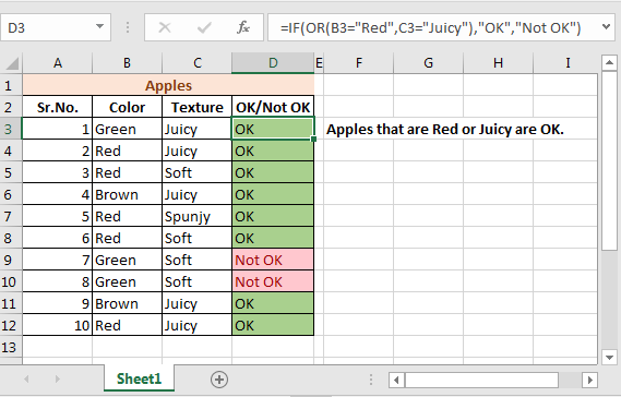
Here we have two conditions and at least one of them need to be true to make you happy. Let’s write an IF OR formula for this in Excel 2016.
Implementation of IF with OR
Generic Formula

=IF(OR(condition1, condition2,…),value if true, value if false)

Example
Let’s consider the example we discussed in the beginning.
We have this table of apple’s colour and type.
If the colour is “Red” or type is “Juicy” then write OK in column D. If the color is not “Red”, nor the type is “Juicy” then type Not OK.

Write this IF OR formula in D2 column and drag it down.

=IF(OR(B3=»Red»,C3=»Juicy»),»OK»,»Not OK»)

And you can see now that only apples that are Red or Juicy are marked OK.

How It Works
IF Statement : You know how IF function in Excel works. It takes a boolean expression as first argument and returns one expression if TRUE and another if FALSE. Learn more about The Excel  IF function.

=IF(TRUE or FALSE, statement if True, statement if false)

OR Function: Checks multiple conditions. Returns TRUE only if at least one of the conditions is TRUE else returns FALSE.

=OR(condition1, condition2,….) ==> TRUE/FALSE

In the end, OR function provides IF function TRUE or FALSE argument and based on that IF prints the result.
Alternate Solution:
Another way to do this is to use nested IFs for Multiple Conditions.

=IF(B3=»Red», “OK”, IF(C3=»Juicy»,”OK”,”Not OK”),”Not OK”)

Nested IF is good when we want different results but not when only one result. It will work but for multiple conditions, it will make your excel formula too long.

So here we learned about how to use IF with OR to check multiple conditions and show results if at least one of all conditions is TRUE. But what if you want to show results only if all condition is true. We will use AND function with IF in excel to do so.

Related Articles:

Excel OR function

Excel AND Function

IF with AND Function in Excel

Excel TRUE Function

Excel NOT function

IF not this or that in Microsoft Excel

IF with AND and OR function in Excel

Popular Articles:

The VLOOKUP Function in Excel

COUNTIF in Excel 2016

How to Use SUMIF Function in Excel

To perform complicated and powerful data analysis, you need to test various conditions at a single point in time. The data analysis might require logical tests also within these multiple conditions.

For this, you need to perform Excel if statement with multiple conditions or ranges that include various If functions in a single formula.

Those who use Excel daily are well versed with Excel If statement as it is one of the most-used formula. Here you can check various Excel If or statement, Nested If, AND function, Excel IF statements, and how to use them. We have also provided a VIDEO TUTORIAL for different If Statements.

There are various If statements available in Excel. You have to know which of the Excel If you will work at what condition. Here you can check multiple conditions where you can use Excel If statement.

1) Excel If Statement

If you want to test a condition to get two outcomes then you can use this Excel If statement.

=If(Marks>=40, “Pass”)

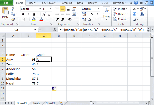
2) Nested If Statement

Let’s take an example that met the below-mentioned condition

• If the score is between 0 to 60, then Grade F
• If the score is between 61 to 70, then Grade D
• If the score is between 71 to 80, then Grade C
• If the score is between 81 to 90, then Grade B
• If the score is between 91 to 100, then Grade A

Then to test the condition the syntax of the formula becomes,

=If(B5<60, “F”,If(B5<71, “D”, If(B5<81,”C”,If(B5<91,”B”,”A”)

3) Excel If with Logical Test

There are 2 different types of conditions AND and OR. You can use the IF statement in excel between two values in both these conditions to perform the logical test.

AND Function: If you are performing the logical test based on AND function, then excel will give you TRUE as an outcome in every condition else it will return false.

OR Function: If you are using OR condition for the logical test, then excel will give you an outcome as TRUE if any of the situations match else it returns false.

For this, multiple testing is to be done using AND and OR function, you should gain expertise in using either or both of these with IF statement. Here we have used if the function with 3 conditions.

How to apply IF & AND function in Excel

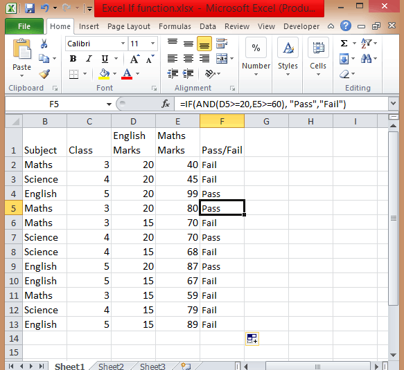
• To perform this multiple if and statements in excel, we will take the data set for the student’s marks that contain fields such as English and Math’s Marks.
• The score of the English subject is stored in the D column whereas the Maths score is stored in column E.
• Let say a student passes the class if his or her score in English is greater than or equal to 20 and he or she scores more than 60 in Maths.
• To create a report in matters of seconds, if formula combined with AND can suffice.
• Type =IF( Excel will display the logical hint just below the cell F2. The parameters of this function are logical_test, value_if_true, value_if_false.
• The first parameter contains the condition to be matched. You can use multiple If and AND conditions combined in this logical test.
• In the second parameter, type the value that you want Excel to display if the condition is true. Similarly, in the third parameter type the value that will be displayed if your condition is false.

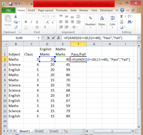
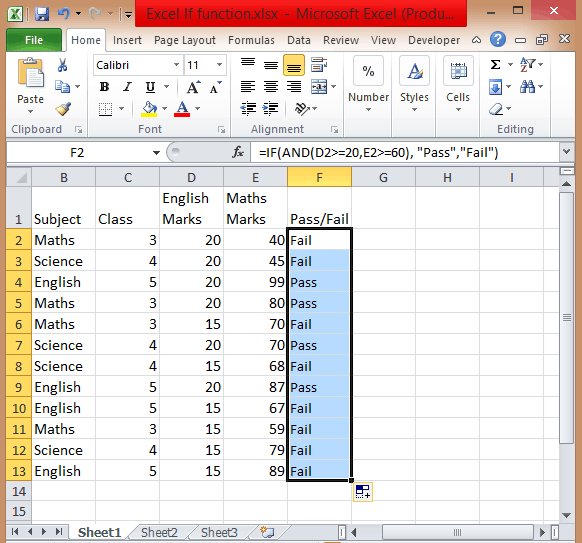
• Apply If & And formula, you will get =IF(AND(D2>=20,E2>=60),”Pass”,”Fail”).

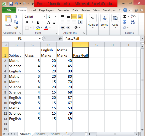
• Add Pass/Fail column in the current table.

• After you have applied this formula, you will find the result in the column.
• Copy the formula from cell F2 and paste in all other cells from F3 to F13.

How to use If with Or function in Excel

To use If and Or statement excel, you need to apply a similar formula as you have applied for If & And with the only difference is that if any of the condition is true then it will show you True.

To apply the formula, you have to follow the above process. The formula is =IF((OR(D2>=20, E2>=60)), “Pass”, “Fail”). If the score is equal or greater than 20 for column D or the second score is equal or greater than 60 then the person is the pass.

How to Use If with And & Or function

If you want to test data based on several multiple conditions then you have to apply both And & Or functions at a single point in time. For example,

Situation 1: If column D>=20 and column E>=60

Situation 2: If column D>=15 and column E>=60

If any of the situations met, then the candidate is passed, else failed. The formula is

=IF(OR(AND(D2>=20, E2>=60), AND(D2>=20, E2>=60)), “Pass”, “Fail”).

4) Excel If Statement with other functions

Above we have learned how to use excel if statement multiple conditions range with And/Or functions. Now we will be going to learn Excel If Statement with other excel functions.

• Excel If with Sum, Average, Min, and Max functions

Let’s take an example where we want to calculate the performance of any student with Poor, Satisfactory, and Good.

If the data set has a predefined structure that will not allow any of the modifications. Then you can add values with this If formula:

=If((A2+B2)>=50, “Good”, If((A2+B2)=>30, “Satisfactory”, “Poor”))

Using the Sum function,

=If(Sum(A2:B2)>=120, “Good”, If(Sum(A2:B2)>=100, “Satisfactory”, “Poor”))

Using the Average function,

=If(Average(A2:B2)>=40, “Good”, If(Average(A2:B2)>=25, “Satisfactory”, “Poor”))

Using Max/Min,

If you want to find out the highest scores, using the Max function. You can also find the lowest scores using the Min function.

=If(C2=Max($C$2:$C$10), “Best result”, “ “)

You can also find the lowest scores using the Min function.

=If(C2=Min($C$2:$C$10), “Worst result”, “ “)

If we combine both these formulas together, then we get

=If(C2=Max($C$2:$C$10), “Best result”, If(C2=Min($C$2:$C$10), “Worst result”, “ “))

You can also call it as nested if functions with other excel functions. To get a result, you can use these if functions with various different functions that are used in excel.

So there are four different ways and types of excel if statements, that you can use according to the situation or condition. Start using it today.

So this is all about Excel If statement multiple conditions ranges, you can also check how to add bullets in excel in our next post.

I hope you found this tutorial useful

You may also like the following Excel tutorials:

• Multiple If Statements in Excel
• Excel Logical test
• How to Compare Two Columns in Excel (using VLOOKUP & IF)
• Using IF Function with Dates in Excel (Easy Examples)