
The IF function allows you to make a logical comparison between a value and what you expect by testing for a condition and returning a result if that condition is True or False.
-
=IF(Something is True, then do something, otherwise do something else)
But what if you need to test multiple conditions, where let’s say all conditions need to be True or False (AND), or only one condition needs to be True or False (OR), or if you want to check if a condition does NOT meet your criteria? All 3 functions can be used on their own, but it’s much more common to see them paired with IF functions.
Use the IF function along with AND, OR and NOT to perform multiple evaluations if conditions are True or False.
Syntax
-
IF(AND()) — IF(AND(logical1, [logical2], …), value_if_true, [value_if_false]))
-
IF(OR()) — IF(OR(logical1, [logical2], …), value_if_true, [value_if_false]))
-
IF(NOT()) — IF(NOT(logical1), value_if_true, [value_if_false]))
|
Argument name |
Description |
|
|
logical_test (required) |
The condition you want to test. |
|
|
value_if_true (required) |
The value that you want returned if the result of logical_test is TRUE. |
|
|
value_if_false (optional) |
The value that you want returned if the result of logical_test is FALSE. |
|
Here are overviews of how to structure AND, OR and NOT functions individually. When you combine each one of them with an IF statement, they read like this:
-
AND – =IF(AND(Something is True, Something else is True), Value if True, Value if False)
-
OR – =IF(OR(Something is True, Something else is True), Value if True, Value if False)
-
NOT – =IF(NOT(Something is True), Value if True, Value if False)
Examples
Following are examples of some common nested IF(AND()), IF(OR()) and IF(NOT()) statements. The AND and OR functions can support up to 255 individual conditions, but it’s not good practice to use more than a few because complex, nested formulas can get very difficult to build, test and maintain. The NOT function only takes one condition.

Here are the formulas spelled out according to their logic:
|
Formula |
Description |
|---|---|
|
=IF(AND(A2>0,B2<100),TRUE, FALSE) |
IF A2 (25) is greater than 0, AND B2 (75) is less than 100, then return TRUE, otherwise return FALSE. In this case both conditions are true, so TRUE is returned. |
|
=IF(AND(A3=»Red»,B3=»Green»),TRUE,FALSE) |
If A3 (“Blue”) = “Red”, AND B3 (“Green”) equals “Green” then return TRUE, otherwise return FALSE. In this case only the first condition is true, so FALSE is returned. |
|
=IF(OR(A4>0,B4<50),TRUE, FALSE) |
IF A4 (25) is greater than 0, OR B4 (75) is less than 50, then return TRUE, otherwise return FALSE. In this case, only the first condition is TRUE, but since OR only requires one argument to be true the formula returns TRUE. |
|
=IF(OR(A5=»Red»,B5=»Green»),TRUE,FALSE) |
IF A5 (“Blue”) equals “Red”, OR B5 (“Green”) equals “Green” then return TRUE, otherwise return FALSE. In this case, the second argument is True, so the formula returns TRUE. |
|
=IF(NOT(A6>50),TRUE,FALSE) |
IF A6 (25) is NOT greater than 50, then return TRUE, otherwise return FALSE. In this case 25 is not greater than 50, so the formula returns TRUE. |
|
=IF(NOT(A7=»Red»),TRUE,FALSE) |
IF A7 (“Blue”) is NOT equal to “Red”, then return TRUE, otherwise return FALSE. |
Note that all of the examples have a closing parenthesis after their respective conditions are entered. The remaining True/False arguments are then left as part of the outer IF statement. You can also substitute Text or Numeric values for the TRUE/FALSE values to be returned in the examples.
Here are some examples of using AND, OR and NOT to evaluate dates.

Here are the formulas spelled out according to their logic:
|
Formula |
Description |
|---|---|
|
=IF(A2>B2,TRUE,FALSE) |
IF A2 is greater than B2, return TRUE, otherwise return FALSE. 03/12/14 is greater than 01/01/14, so the formula returns TRUE. |
|
=IF(AND(A3>B2,A3<C2),TRUE,FALSE) |
IF A3 is greater than B2 AND A3 is less than C2, return TRUE, otherwise return FALSE. In this case both arguments are true, so the formula returns TRUE. |
|
=IF(OR(A4>B2,A4<B2+60),TRUE,FALSE) |
IF A4 is greater than B2 OR A4 is less than B2 + 60, return TRUE, otherwise return FALSE. In this case the first argument is true, but the second is false. Since OR only needs one of the arguments to be true, the formula returns TRUE. If you use the Evaluate Formula Wizard from the Formula tab you’ll see how Excel evaluates the formula. |
|
=IF(NOT(A5>B2),TRUE,FALSE) |
IF A5 is not greater than B2, then return TRUE, otherwise return FALSE. In this case, A5 is greater than B2, so the formula returns FALSE. |

Using AND, OR and NOT with Conditional Formatting
You can also use AND, OR and NOT to set Conditional Formatting criteria with the formula option. When you do this you can omit the IF function and use AND, OR and NOT on their own.
From the Home tab, click Conditional Formatting > New Rule. Next, select the “Use a formula to determine which cells to format” option, enter your formula and apply the format of your choice.

Using the earlier Dates example, here is what the formulas would be.

|
Formula |
Description |
|---|---|
|
=A2>B2 |
If A2 is greater than B2, format the cell, otherwise do nothing. |
|
=AND(A3>B2,A3<C2) |
If A3 is greater than B2 AND A3 is less than C2, format the cell, otherwise do nothing. |
|
=OR(A4>B2,A4<B2+60) |
If A4 is greater than B2 OR A4 is less than B2 plus 60 (days), then format the cell, otherwise do nothing. |
|
=NOT(A5>B2) |
If A5 is NOT greater than B2, format the cell, otherwise do nothing. In this case A5 is greater than B2, so the result will return FALSE. If you were to change the formula to =NOT(B2>A5) it would return TRUE and the cell would be formatted. |
Note: A common error is to enter your formula into Conditional Formatting without the equals sign (=). If you do this you’ll see that the Conditional Formatting dialog will add the equals sign and quotes to the formula — =»OR(A4>B2,A4<B2+60)», so you’ll need to remove the quotes before the formula will respond properly.
Need more help?

See also
You can always ask an expert in the Excel Tech Community or get support in the Answers community.
Learn how to use nested functions in a formula
IF function
AND function
OR function
NOT function
Overview of formulas in Excel
How to avoid broken formulas
Detect errors in formulas
Keyboard shortcuts in Excel
Logical functions (reference)
Excel functions (alphabetical)
Excel functions (by category)
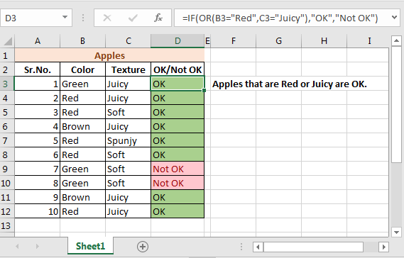
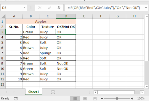
A fruit seller is selling apples. You will buy apples only if they are Red or Juicy. If an apple is not Red nor Juicy, you will not buy it.
Here we have two conditions and at least one of them need to be true to make you happy. Let’s write an IF OR formula for this in Excel 2016.
Implementation of IF with OR
Generic Formula
=IF(OR(condition1, condition2,…),value if true, value if false)
Example
Let’s consider the example we discussed in the beginning.
We have this table of apple’s colour and type.
If the colour is “Red” or type is “Juicy” then write OK in column D. If the color is not “Red”, nor the type is “Juicy” then type Not OK.

Write this IF OR formula in D2 column and drag it down.
=IF(OR(B3=»Red»,C3=»Juicy»),»OK»,»Not OK»)
And you can see now that only apples that are Red or Juicy are marked OK.
How It Works
IF Statement : You know how IF function in Excel works. It takes a boolean expression as first argument and returns one expression if TRUE and another if FALSE. Learn more about The Excel IF function.
=IF(TRUE or FALSE, statement if True, statement if false)
OR Function: Checks multiple conditions. Returns TRUE only if at least one of the conditions is TRUE else returns FALSE.
=OR(condition1, condition2,….) ==> TRUE/FALSE
In the end, OR function provides IF function TRUE or FALSE argument and based on that IF prints the result.
Alternate Solution:
Another way to do this is to use nested IFs for Multiple Conditions.
=IF(B3=»Red», “OK”, IF(C3=»Juicy»,”OK”,”Not OK”),”Not OK”)
Nested IF is good when we want different results but not when only one result. It will work but for multiple conditions, it will make your excel formula too long.
So here we learned about how to use IF with OR to check multiple conditions and show results if at least one of all conditions is TRUE. But what if you want to show results only if all condition is true. We will use AND function with IF in excel to do so.
Related Articles:
Excel OR function
Excel AND Function
IF with AND Function in Excel
Excel TRUE Function
Excel NOT function
IF not this or that in Microsoft Excel
IF with AND and OR function in Excel
Popular Articles:
The VLOOKUP Function in Excel
COUNTIF in Excel 2016
How to Use SUMIF Function in Excel
In this tutorial, we will learn about the IF function in Excel. Along with IF, the AND and OR functions are important formulas too. A nested IF simply means multiple IF functions in a single syntax.
Introducing IF Function in Excel
Let’s get started with this easy guide to using the IF function and all its related functions in Microsoft Excel, step-by-step with supporting images and examples.
1. IF Function
To learn to use the IF function, we will take an example of a mark list of students below.

Our goal is to find out which student has passed or failed and what are their grades. Of course, it would be a tedious task to find out pass or fail results and grades for each student in this list.
To ease our task, we have IF functions for that matter. The IF function will automatically identify if a student has passed or failed based on the criteria you provide to it.
It will automatically mark a student as “Pass” if he/she has scored above the minimum pass mark and mark a student as “Fail” if he/she has scored below the minimum pass mark.
The IF function automatically assigns the appropriate grades to students based on their marks if you command it.
Here is a glimpse of how the IF function helps you out with assigning grades and marking “Pass” or “Fail”.

Steps to use IF function in Excel
We have allotted certain grades and marked them as Pass or Fail to students based on the percentages they have secured in their exams, with the help of the IF function.
1. Using the IF function in Excel to identify passed/failed students
Let’s learn how we can use the IF formula to achieve this. We will use the same example. We take the minimum passing percentage as 34%.

- Find out the percentage of total marks of every student.
- Create a new column named “Pass/Fail”.
- In the blank cell below the title, type the IF formula as follows next.
- Type =IF( and select the first student’s percentage and type >=34.
- Put a comma and move to the next argument named [value_if_true]. This means you’re being asked to put a value to be displayed if the above condition is true. Remember these arguments are case sensitive.
- Once you have put a comma, type “Pass”.
- Put a comma and move to the next argument named [value_if_false] to display a value when the above condition is false. This field is optional in most cases but we need a false value because it is a mark list.
- Close the bracket and hit ENTER.

You can see that the formula is displaying “Pass” for the first student because she has secured above 34%.
- Double-click or drag the cell from the right corner below to autofill the formula to all the students below.

Recommended read: How to Autofill in Excel?
2. Nested IF Function
Now, let us start assigning grades to all students.
We are going to be using multiple IF functions in a single syntax this time to provide multiple criteria to the IF function. This is called Nested IF in Excel.
However, there is no specific function named “Nested IF” in Excel, it is simply that this behavior has been given a name i.e., Nested IF.
Before we proceed further, we need to first make a table that displays a grading class for each grade. Here is an example below.

- Create a new column named “Grade”.
- Type the IF function in a blank cell below the title as follows.
- Type =IF( and now type AE118>=85,”A”,IF(AE118>=70,”B”,IF(AE118>=55,”C”,IF(AE118>=34,”D”,IF(AE118<=33,”Fail”.

- Note that AE118 is our cell address for the first student’s percentage. It will be different in your case. Refer to the image above to make sense of the formula.
- The formula simply states- if percentage marks are above and equal to 85 then give “A”, if percentage marks are above and equal to 70 then give “B”, and so on and so forth. For the last condition, we have applied the condition- if the marks are less than or equal to 33 then give “Fail”.
- For the last IF statement, you can either put the result as “Fail” or “E” as you like.
- Now, note that we will close the formula with 5 brackets for this example as we have used a total of 5 IF formulas.

- Hit ENTER to complete the formula.

You can now see that the formula has been applied to the first entry and the result is B because the student has secured 72.5% which is less than 75%. This means the nested Ifs are working correctly.
- Now drag the cell from the lower right corner to autofill the formula to the rest of the entries.

You can see that we now have grades and pass/fail markings for every student on the list successfully.
3. IF with AND in Excel
Let us learn the IF formula with the AND function in a single syntax with a minor example.

When you have two or more distinct conditions to be used together, you can use the IF function with AND in Excel.
While nested IFs will also work, using AND function will save your time as it is shorter to type. So, let’s get started.
Our goal is to identify currencies with revenues greater than 20,000 and less than 50,000 and mark them as “Good”.
- Type =IF(AND( because we are using the IF with AND function.
- Select the first cell under Revenue, and type >20000.
- Put a comma and select the first cell under Revenue again and type <50000.
- Now, close the bracket to complete the AND function. We’re still working on the IF function so do not put two brackets.
- We come back to the IF function as soon as we close the AND function. Now put the values to be displayed if the condition is true or false.
- Put a comma to move to the argument [value_if_true] and type “Good”.
- You can provide a result in the [value_if_false] argument, but it is completely optional. If nothing is provided then the cells will display FALSE if the condition is false. But if you want the cells to remain blank simply put “” (two double quotation marks) in this argument.
- Close the bracket to complete the IF function as well.

This is how the syntax should look like before pressing ENTER.
- Hit ENTER to view results and drag the cell down to autofill the formula to the rest of the cells.

There are only two such cells for which the condition is true and the result is being displayed as “Good” for them and the rest of the cells are blank. This means the formula is working correctly.
4. IF with OR in Excel
Using the OR function with the IF function will give results for either of the conditions that are true.
- Type =IF(OR(.
- Select the first cell under Revenue and type >=20000.
- Put a comma and select the first cell under Revenue again and type <=50000.
- Now, close the bracket to complete the OR function. We’re still working on the IF function so do not put two brackets.
- Coming back to the IF function, we now put the values to be displayed if the condition is true or false.
- Put a comma to move to the argument [value_if_true] and type “Flag”.
- Put a comma to move to the argument [value_if_false] and type “”.

This is how the syntax should look like before pressing ENTER.
- Close the bracket to complete the OR function and hit ENTER.
- Drag the cell below to get the results for the rest.

The formula is true for all entries and so it is displaying “Flag” for all of them. This is because all the values are either lower than 50,000 or greater than 20,000.
Conclusion
This was all about IF functions and other related functions to the IF function that are AND and OR functions.
Reference: ExcelJet
Nesting functions in Excel refers to placing one function inside another. The nested function acts as one of the main function’s arguments. The AND, OR, and IF functions are some of Excel’s better known logical functions that are commonly used together.
Instructions in this article apply to Excel 2019, 2016, 2013, 2010, 2007; Excel for Microsoft 365, Excel Online, and Excel for Mac.
Build the Excel IF Statement
When using the IF, AND, and OR functions, one or all of the conditions must be true for the function to return a TRUE response. If not, the function returns FALSE as a value.
For the OR function (see row 2 in the image below), if one of these conditions is true, the function returns a value of TRUE. For the AND function (see row 3), all three conditions must be true for the function to returns a value of TRUE.
In the image below, rows 4 to 6 contain formulas where the AND and OR functions are nested inside the IF function.
When the AND and OR functions are combined with the IF function, the resulting formula has much greater capabilities.
In this example, three conditions are tested by the formulas in rows 2 and 3:
- Is the value in cell A2 less than 50?
- Is the value in cell A3 not equal to 75?
- Is the value in cell A4 greater than or equal to 100?
Also, in all of the examples, the nested function acts as the IF function’s first argument. This first element is known as the Logical_test argument.
=IF(OR(A2<50,A3<>75,A4>=100),"Data Correct","Data Error")
=IF(AND(A2<50,A3<>75,A4>=100),1000,TODAY())
Change the Formula’s Output
In all formulas in rows 4 to 6, the AND and OR functions are identical to their counterparts in rows 2 and 3 in that they test the data in cells A2 to A4 to see if it meets the required condition.
The IF function is used to control the formula’s output based on what is entered for the function’s second and third arguments. Examples of this output can be text as seen in row 4, a number as seen in row 5, the output from the formula, or a blank cell.
In the case of the IF/AND formula in cell B5, since not all three cells in the range A2 to A4 are true — the value in cell A4 is not greater than or equal to 100 — the AND function returns a FALSE value. The IF function uses this value and returns its Value_if_false argument — the current date supplied by the TODAY function.
On the other hand, the IF/OR formula in row four returns the text statement Data Correct for one of two reasons:
-
The OR value has returned a TRUE value — the value in cell A3 does not equal 75.
-
The IF function then used this result to return its Value_if_false argument: Data Correct.
Use the IF Statement in Excel
The next steps cover how to enter the IF/OR formula located in cell B4 from the example. These same steps can be used to enter any of the IF formulas in these examples.
There are two ways to enter formulas in Excel. Either type the formula in the Formula Bar or use the Function Arguments dialog box. The dialog box takes care of the syntax such as placing comma separators between arguments and surrounding text entries in quotation marks.
The steps used to enter the IF/OR formula in cell B4 are as follows:
-
Select cell B4 to make it the active cell.
-
On the ribbon, go to Formulas.
-
Select Logical to open the function dropdown list.
-
Choose IF in the list to open the Function Arguments dialog box.
-
Place the cursor in the Logical_test text box.
-
Enter the complete OR function:
OR(A2<50,A3<>75,A4>=100)
-
Place the cursor in the Value_if_true text box.
-
Type Data Correct.
-
Place the cursor in the Value_if_false text box.
-
Type Data Error.
-
Select OK to complete the function.
-
The formula displays the Value_if_true argument of Data Correct.
-
Select cell B4 to see the complete function in the formula bar above the worksheet.
Thanks for letting us know!
Get the Latest Tech News Delivered Every Day
Subscribe