
The IF function allows you to make a logical comparison between a value and what you expect by testing for a condition and returning a result if that condition is True or False.
-
=IF(Something is True, then do something, otherwise do something else)
But what if you need to test multiple conditions, where let’s say all conditions need to be True or False (AND), or only one condition needs to be True or False (OR), or if you want to check if a condition does NOT meet your criteria? All 3 functions can be used on their own, but it’s much more common to see them paired with IF functions.
Use the IF function along with AND, OR and NOT to perform multiple evaluations if conditions are True or False.
Syntax
-
IF(AND()) — IF(AND(logical1, [logical2], …), value_if_true, [value_if_false]))
-
IF(OR()) — IF(OR(logical1, [logical2], …), value_if_true, [value_if_false]))
-
IF(NOT()) — IF(NOT(logical1), value_if_true, [value_if_false]))
|
Argument name |
Description |
|
|
logical_test (required) |
The condition you want to test. |
|
|
value_if_true (required) |
The value that you want returned if the result of logical_test is TRUE. |
|
|
value_if_false (optional) |
The value that you want returned if the result of logical_test is FALSE. |
|
Here are overviews of how to structure AND, OR and NOT functions individually. When you combine each one of them with an IF statement, they read like this:
-
AND – =IF(AND(Something is True, Something else is True), Value if True, Value if False)
-
OR – =IF(OR(Something is True, Something else is True), Value if True, Value if False)
-
NOT – =IF(NOT(Something is True), Value if True, Value if False)
Examples
Following are examples of some common nested IF(AND()), IF(OR()) and IF(NOT()) statements. The AND and OR functions can support up to 255 individual conditions, but it’s not good practice to use more than a few because complex, nested formulas can get very difficult to build, test and maintain. The NOT function only takes one condition.

Here are the formulas spelled out according to their logic:
|
Formula |
Description |
|---|---|
|
=IF(AND(A2>0,B2<100),TRUE, FALSE) |
IF A2 (25) is greater than 0, AND B2 (75) is less than 100, then return TRUE, otherwise return FALSE. In this case both conditions are true, so TRUE is returned. |
|
=IF(AND(A3=»Red»,B3=»Green»),TRUE,FALSE) |
If A3 (“Blue”) = “Red”, AND B3 (“Green”) equals “Green” then return TRUE, otherwise return FALSE. In this case only the first condition is true, so FALSE is returned. |
|
=IF(OR(A4>0,B4<50),TRUE, FALSE) |
IF A4 (25) is greater than 0, OR B4 (75) is less than 50, then return TRUE, otherwise return FALSE. In this case, only the first condition is TRUE, but since OR only requires one argument to be true the formula returns TRUE. |
|
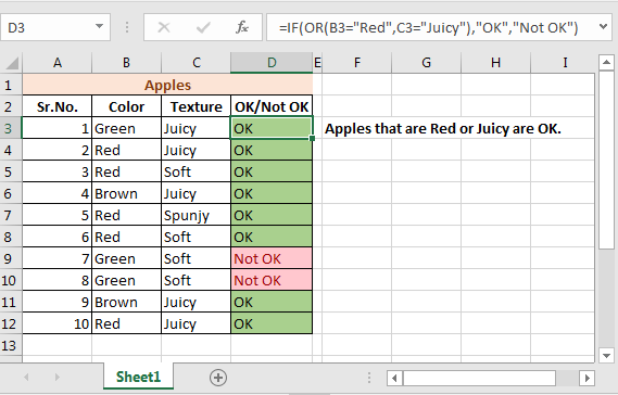
=IF(OR(A5=»Red»,B5=»Green»),TRUE,FALSE) |
IF A5 (“Blue”) equals “Red”, OR B5 (“Green”) equals “Green” then return TRUE, otherwise return FALSE. In this case, the second argument is True, so the formula returns TRUE. |
|
=IF(NOT(A6>50),TRUE,FALSE) |
IF A6 (25) is NOT greater than 50, then return TRUE, otherwise return FALSE. In this case 25 is not greater than 50, so the formula returns TRUE. |
|
=IF(NOT(A7=»Red»),TRUE,FALSE) |
IF A7 (“Blue”) is NOT equal to “Red”, then return TRUE, otherwise return FALSE. |
Note that all of the examples have a closing parenthesis after their respective conditions are entered. The remaining True/False arguments are then left as part of the outer IF statement. You can also substitute Text or Numeric values for the TRUE/FALSE values to be returned in the examples.
Here are some examples of using AND, OR and NOT to evaluate dates.

Here are the formulas spelled out according to their logic:
|
Formula |
Description |
|---|---|
|
=IF(A2>B2,TRUE,FALSE) |
IF A2 is greater than B2, return TRUE, otherwise return FALSE. 03/12/14 is greater than 01/01/14, so the formula returns TRUE. |
|
=IF(AND(A3>B2,A3<C2),TRUE,FALSE) |
IF A3 is greater than B2 AND A3 is less than C2, return TRUE, otherwise return FALSE. In this case both arguments are true, so the formula returns TRUE. |
|
=IF(OR(A4>B2,A4<B2+60),TRUE,FALSE) |
IF A4 is greater than B2 OR A4 is less than B2 + 60, return TRUE, otherwise return FALSE. In this case the first argument is true, but the second is false. Since OR only needs one of the arguments to be true, the formula returns TRUE. If you use the Evaluate Formula Wizard from the Formula tab you’ll see how Excel evaluates the formula. |
|
=IF(NOT(A5>B2),TRUE,FALSE) |
IF A5 is not greater than B2, then return TRUE, otherwise return FALSE. In this case, A5 is greater than B2, so the formula returns FALSE. |

Using AND, OR and NOT with Conditional Formatting
You can also use AND, OR and NOT to set Conditional Formatting criteria with the formula option. When you do this you can omit the IF function and use AND, OR and NOT on their own.
From the Home tab, click Conditional Formatting > New Rule. Next, select the “Use a formula to determine which cells to format” option, enter your formula and apply the format of your choice.

Using the earlier Dates example, here is what the formulas would be.

|
Formula |
Description |
|---|---|
|
=A2>B2 |
If A2 is greater than B2, format the cell, otherwise do nothing. |
|
=AND(A3>B2,A3<C2) |
If A3 is greater than B2 AND A3 is less than C2, format the cell, otherwise do nothing. |
|
=OR(A4>B2,A4<B2+60) |
If A4 is greater than B2 OR A4 is less than B2 plus 60 (days), then format the cell, otherwise do nothing. |
|
=NOT(A5>B2) |
If A5 is NOT greater than B2, format the cell, otherwise do nothing. In this case A5 is greater than B2, so the result will return FALSE. If you were to change the formula to =NOT(B2>A5) it would return TRUE and the cell would be formatted. |
Note: A common error is to enter your formula into Conditional Formatting without the equals sign (=). If you do this you’ll see that the Conditional Formatting dialog will add the equals sign and quotes to the formula — =»OR(A4>B2,A4<B2+60)», so you’ll need to remove the quotes before the formula will respond properly.
Need more help?

See also
You can always ask an expert in the Excel Tech Community or get support in the Answers community.
Learn how to use nested functions in a formula
IF function
AND function
OR function
NOT function
Overview of formulas in Excel
How to avoid broken formulas
Detect errors in formulas
Keyboard shortcuts in Excel
Logical functions (reference)
Excel functions (alphabetical)
Excel functions (by category)
Purpose
Test multiple conditions with OR
Return value
TRUE if any arguments evaluate TRUE; FALSE if not.
Usage notes
The OR function returns TRUE if any given argument evaluates to TRUE, and returns FALSE only if all supplied arguments evaluate to FALSE. The OR function can be used as the logical test inside the IF function to avoid nested IFs, and can be combined with the AND function.
The OR function is used to check more than one logical condition at the same time, up to 255 conditions, supplied as arguments. Each argument (logical1, logical2, etc.) must be an expression that returns TRUE or FALSE or a value that can be evaluated as TRUE or FALSE. The arguments provided to the OR function can be constants, cell references, arrays, or logical expressions.
The purpose of the OR function is to evaluate more than one logical test at the same time and return TRUE if any result is TRUE. For example, if A1 contains the number 50, then:
=OR(A1>0,A1>75,A1>100) // returns TRUE
=OR(A1<0,A1=25,A1>100) // returns FALSE
The OR function will evaluate all values supplied and return TRUE if any value evaluates to TRUE. If all logicals evaluate to FALSE, the OR function will return FALSE. Note: Excel will evaluate any number except zero (0) as TRUE.
Both the AND function and the OR function will aggregate results to a single value. This means they can’t be used in array operations that need to deliver an array of results. To work around this limitation, you can use Boolean logic. For more information, see: Array formulas with AND and OR logic.
Examples
For example, to test if the value in A1 OR the value in B1 is greater than 75, use the following formula:
=OR(A1>75,B1>75)
OR can be used to extend the functionality of functions like the IF function. Using the above example, you can supply OR as the logical_test for an IF function like so:
=IF(OR(A1>75,B1>75), "Pass", "Fail")
This formula will return «Pass» if the value in A1 is greater than 75 OR the value in B1 is greater than 75.
Array form
If you enter OR as an array formula, you can test all values in a range against a condition. For example, this array formula will return TRUE if any cell in A1:A100 is greater than 15:
=OR(A1:A100>15)
Note: In Legacy Excel, this is an array formula and must be entered with control + shift + enter.
Notes
- Each logical condition must evaluate to TRUE or FALSE, or be arrays or references that contain logical values.
- Text values or empty cells supplied as arguments are ignored.
- The OR function will return #VALUE if no logical values are found
Функция OR (ИЛИ) в Excel используется для сравнения двух условий.
Содержание
- Что возвращает функция
- Синтаксис
- Аргументы функции
- Дополнительная информация
- Примеры использования функции OR (ИЛИ) в Excel
- Пример 1. Используем аргументы TRUE и FALSE в функции OR (ИЛИ)
- Пример 2. Используем ссылки на ячейки, содержащих TRUE/FALSE
- Пример 3. Используем условия с функцией OR (ИЛИ)
- Пример 4. Используем числовые значения с функцией OR (ИЛИ)
- Пример 5. Используем функцию OR (ИЛИ) с другими функциями
Что возвращает функция
Возвращает логическое значение TRUE (Истина), при выполнении условий сравнения в функции и отображает FALSE (Ложь), если условия функции не совпадают.
Синтаксис
=OR(logical1, [logical2],…) — английская версия
=ИЛИ(логическое_значение1;[логическое значение2];…) — русская версия
Аргументы функции
- logical1 (логическое_значение1) — первое условие которое оценивает функция по логике TRUE или FALSE;
- [logical2] ([логическое значение2]) — (не обязательно) это второе условие которое вы можете оценить с помощью функции по логике TRUE или FALSE.
Дополнительная информация
- Функция OR (ИЛИ) может использоваться с другими формулами.
Например, в функции IF (ЕСЛИ) вы можете оценить условие и затем присвоить значение, когда данные отвечают условиям логики TRUE или FALSE. Используя функцию вместе с IF (ЕСЛИ), вы можете тестировать несколько условий оценки значений за раз.
Например, если вы хотите проверить значение в ячейке А1 по условию: “Если значение больше “0” или меньше “100” то… “ — вы можете использовать следующую формулу:
=IF(OR(A1>100,A1<0),”Верно”,”Неверно”) — английская версия
=ЕСЛИ(ИЛИ(A1>100;A1<0);»Верно»;»Неверно») — русская версия
- Аргументы функции должны быть логически вычислимы по принципу TRUE или FALSE;
- Текст и пустые ячейки игнорируются функцией;
- Если вы используете функцию с не логически вычисляемыми значениями — она выдаст ошибку;
- Вы можете тестировать максимум 255 условий в одной формуле.
Примеры использования функции OR (ИЛИ) в Excel
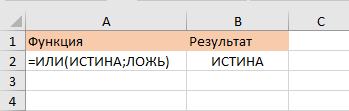
Пример 1. Используем аргументы TRUE и FALSE в функции OR (ИЛИ)

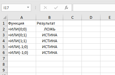
Вы можете использовать TRUE/FALSE в качестве аргументов. Если любой из них соответствует условию TRUE, функция выдаст результат TRUE. Если оба аргумента функции соответствуют условию FALSE, функция выдаст результат FALSE.
Больше лайфхаков в нашем Telegram Подписаться
Она может использовать аргументы TRUE и FALSE в кавычках.
Пример 2. Используем ссылки на ячейки, содержащих TRUE/FALSE
Вы можете использовать ссылки на ячейки со значениями TRUE или FALSE. Если любое значение из ссылок соответствует условиям TRUE, функция выдаст TRUE.
Пример 3. Используем условия с функцией OR (ИЛИ)
Вы можете проверять условия с помощью функции OR (ИЛИ). Если любое из условий соответствует TRUE, функция выдаст результат TRUE.
Пример 4. Используем числовые значения с функцией OR (ИЛИ)
Число “0” считается FALSE в Excel по умолчанию. Любое число, выше “0”, считается TRUE (оно может быть положительным, отрицательным или десятичным числом).
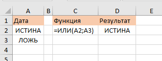
Пример 5. Используем функцию OR (ИЛИ) с другими функциями
Вы можете использовать функцию OR (ИЛИ) с другими функциями для того, чтобы оценить несколько условий.
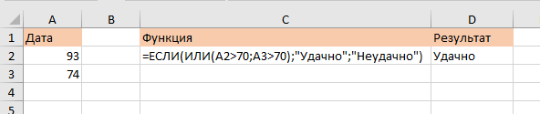
На примере ниже показано, как использовать функцию вместе с IF (ЕСЛИ):
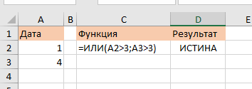
На примере выше, мы дополнительно используем функцию IF (ЕСЛИ) для того, чтобы проверить несколько условий. Формула проверяет значение ячеек А2 и A3. Если в одной из них значение более чем “70”, то формула выдаст “TRUE”.
What is OR Function in Excel?
The OR function of Excel is used to test multiple conditions at the same time. A condition is an expression that evaluates to either “true” or “false” but not to both simultaneously. The OR function is categorized as a Logical function of Excel.
It returns either of the following outcomes:
- True, if any of the conditions is true or all the conditions are true
- False, if all the conditions are false
For example, the formula “=OR(2>4,8>5)” (ignore the double quotation marks) returns “true.” The first condition (2>4) evaluates to false, while the second condition (8>5) evaluates to true. Since one of the conditions is true, the final output is “true.”
A condition is supplied as an argument to the OR function. An argument can consist of numbers, text strings, cell references, formulas or Boolean values (true and false). The purpose of using the OR function is to assess whether any of the various conditions is met or not. It also facilitates multiple comparisons of data values.
Table of contents
- What is OR Function in Excel?
- Syntax of the OR Function of Excel
- Example #1–Test Two Conditions Containing Numeric Values
- Example #2–Test Two Conditions Containing a mix of Numerical and Textual Values
- Example #3–Test Three Conditions Containing a mix of Numerical and Textual Values
- Example #4–Test Three Conditions With a Nested OR or Nested AND Within the IF Function
- Frequently Asked Questions
- Recommended Articles
- Syntax of the OR Function of Excel
Syntax of the OR Function of Excel
The syntax of the OR function in excel is given in the following image:

The OR function accepts the following arguments:
- Logical1: This is the first condition to be tested.
- Logical2: This is the second condition to be tested.
“Logical1” is required, while “logical2” and the subsequent “logical” arguments are optional.
The OR function can be used either alone or in combination with the IF function of Excel. The benefits of using the OR function are expanded when it is combined with the AND and IF functions of ExcelIF function in Excel evaluates whether a given condition is met and returns a value depending on whether the result is “true” or “false”. It is a conditional function of Excel, which returns the result based on the fulfillment or non-fulfillment of the given criteria.
read more. For such combinations, the OR and/or AND functionsThe AND function in Excel is classified as a logical function; it returns TRUE if the specified conditions are met, otherwise it returns FALSE.read more can be nested within the IF function.
Let us consider some examples to understand the working of the OR function of Excel. To know more about the nested OR function, refer to example #4 of this article.
Note 1: Each argument (condition) of the OR function must necessarily evaluate to either “true” or “false.” Moreover, each condition should consist of the relevant logical (or comparison) operator. There are six logical operators in ExcelLogical operators in excel are also known as the comparison operators and they are used to compare two or more values, the return output given by these operators are either true or false, we get true value when the conditions match the criteria and false as a result when the conditions do not match the criteria.read more. These are “equal to” (=), “not equal to” (<>), “greater than” (>), “greater than or equal to” (>=), “less than” (<), and “less than or equal to” (<=).
Note 2: A maximum of 255 conditions can be tested in Excel 2007 and the newer versions. In the earlier versions of Excel, a total of 30 conditions can be tested.
You can download this OR Function Excel Template here – OR Function Excel Template
Example #1–Test Two Conditions Containing Numeric Values
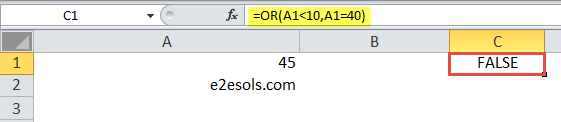
The succeeding image shows a number and the name of an unavailable website in cells A1 and A2 respectively. With the help of the OR function of Excel, evaluate the following conditions together:
- The value of cell A1 is less than 10
- The value of cell A1 is equal to 40
The steps to test the given conditions by using the OR function in excel are listed as follows:
Step 1: Insert the required logical operators in the given conditions. So, enter the following formula in cell C1.
“=OR(A1<10,A1=40)”
Here, the first condition is A1<10 and the second condition is A1=40.
Step 2: Press the “Enter” key. The output in cell C1 is “false.” This is because both the given conditions are false. Neither the value of cell A1 is less than 10, nor is it equal to 40.
The formula and the output are shown in the following image.
Example #2–Test Two Conditions Containing a mix of Numerical and Textual Values
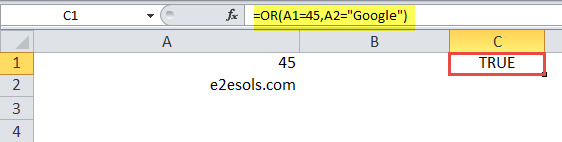
Working on the dataset of example #1, we want to evaluate the following conditions together:
- The value of cell A1 is equal to 45
- The value of cell A2 is “Google.”
Use the OR function of Excel.
The steps to test the given conditions with the help of the OR function are listed as follows:
Step 1: Enter the following formula in cell C1.
“=OR(A1=45,A2=“Google”)”
We have inserted the appropriate logical operators in the given conditions. So, the first condition is A1=45 and the second condition is A2=“Google.”
Step 2: Press the “Enter” key. The output appears as “true” in cell C1.
In this example, the first condition is true as the value of cell A1 is equal to 45. The second condition is false as the value of cell A2 is not “Google.” Since one of the two conditions evaluate to true, the final output is “true.”
The formula and the output are shown in the following image.
Example #3–Test Three Conditions Containing a mix of Numerical and Textual Values
Working on the dataset of example #1, evaluate the following three conditions together:
- The value of cell A1 is greater than or equal to 5
- The value of cell A1 is equal to 35
- The value of cell A2 is “e2esols.com.”
Use the OR function of Excel.
The steps to test the given conditions by using the OR function in excel are listed as follows:
Step 1: Insert the logical operators that fit the given conditions. So, enter the following formula in cell C1.
“=OR(A1>=5,A1=35,A2=“e2esols.com”)”
Here, the first, second, and third conditions are “A1>=5,” “A1=35,” and A2=“e2esols.com” respectively.
Step 2: Press the “Enter” key. The output in cell C1 is “true.”
The first condition evaluates to true because 45 (value of cell A1) is certainly greater than 5. The second condition is false as 45 is not equal to 35. The third condition is true as the value of cell A2 is “e2esols.com.”
So, two out of three conditions are true. Consequently, the final output is also “true.” Even if one of the three conditions had been true, the final output would still have been “true.”
The formula (entered in step 1) and the output are shown in the following image.

Example #4–Test Three Conditions With a Nested OR or Nested AND Within the IF Function
The succeeding table shows some random numbers in column A. In column B, the following three conditions are tested:
- The value of cell A2 is less than 50
- The value of cell A3 is not equal to 75
- The value of cell A4 is greater than or equal to 100
The preceding conditions have been tested by using the following functions (in the given sequence):
- OR function
- AND function
- IF and OR functions
- IF and AND functionsThe IF AND excel formula is the combination of two different logical functions often nested together that enables the user to evaluate multiple conditions using AND functions. Based on the output of the AND function, the IF function returns either the “true” or “false” value, respectively.
read more
Column C shows the outputs obtained by each formula of column B. The row numbers are displayed under the label “Sr. No,” which stands for serial number.
Consider each column and row of the table as the respective column and row of an Excel worksheet.
| Sr. No | A | B | C |
|---|---|---|---|
| 1 | DATA | FORMULAS APPLIED | RESULTS |
| 2 | 50 | =OR(A2<50,A3<>75,A4>=100) | TRUE |
| 3 | 25 | =AND(A2<50,A3<>75,A4>=100) | FALSE |
| 4 | 99 | =IF(OR(A2<50,A3<>75,A4>=100),”Data Error”,”Data Correct”) | Data Error |
| 5 | =IF(AND(A2<50,A3<>75,A4>=100),”Data Error”,”Data Correct”) | Data Correct |
The conditions tested in column B and their outcomes are listed as follows:
- A2<50: It evaluates to false as the value of cell A2 (50) is not less than 50.
- A3<>75: It evaluates to true because the value of cell A3 (25) is not equal to 75.
- A4>=100: It evaluates to false as the value of cell A4 (99) is neither greater than nor equal to 100.
The rows of column B are explained as follows:
Row 2: In this row, the three preceding conditions are tested (in cell B2) using the OR excel function. Since one of the three conditions is true, the final output of the OR function (in cell C2) is “true.”
Row 3: In this row, the three preceding conditions are tested (in cell B3) using the AND function. Since two out of three conditions are false, the final output of the AND function (in cell C3) is “false.”
Row 4: In this row, the given conditions are evaluated (in cell B4) using the nested OR function. Since the output of the OR function is “true” (as explained for row 2), the IF function considers that the logical test (condition) has been met. Consequently, the IF function returns the string defined as the “value_if_true” argument, which is “data error” (in cell C4).
Row 5: In this row, the three stated conditions are evaluated (in cell B5) using the nested AND function. The AND function returns the output “false” (as explained for row 3). So, the IF function realizes that the logical test has not been met. As a result, the IF function returns the string “data correct” (in cell C5), which is the “value_if_false” argument.
Note 1: The AND function returns “true” if all the tested conditions evaluate to true. It returns “false” if any of the conditions evaluate to false. Like the OR function, the AND function is also a logical function of Excel.
Note 2: In nesting functions, one function is placed inside another function. The function that is inside is known as a nested function. Excel calculates the nested function first, followed by the outer function. The output of the nested function is used as an argument of the outer function.
Frequently Asked Questions
1. State whether Excel has an OR function or not. If yes, define it.
Yes, Excel does have an OR function. The OR function is available in all versions of Excel. However, there are certain limitations related to the number of conditions that can be tested with the OR function.
Multiple conditions can be tested simultaneously by using the OR function of Excel. It is a logical function of Excel, which returns either of the two Boolean values (true and false) as the outcome. The OR function returns “true” if any or all conditions are true. It returns “false” if all conditions are false.
Note: For the meaning of condition and the number of conditions that can be tested, refer to the introduction and syntax discussed in this article.
2. How is the OR function of Excel used with the conditional formatting feature of Excel?
The steps to use the OR function with the conditional formatting feature are listed as follows:
a. Select the range on which conditional formatting needs to be applied.
b. From the Home tab, click the “conditional formatting” drop-down from the “styles” group. Select “new rule.”
c. The “new formatting rule” window opens. Choose the option “use a formula to determine which cells to format” under “select a rule type.”
d. Under “format values where this formula is true,” enter the OR formula. For instance, in the range A2:A10, if the numbers greater than 30 or equal to 25 need to be formatted, enter the formula “=OR(A2>30,A2=25)” (without the beginning and ending double quotation marks).
e. Click “format” and select a color from the “fill” tab. Click “Ok” to proceed.
f. Click “Ok” again in the “new formatting rule” window.
The cells of the selected range, for which either of the two conditions (A2>30,A2=25) is true, are colored. The cells, for which both conditions are false, are not colored.
Note 1: When a conditional formatting rule is applied using the OR function, every cell is checked for multiple conditions entered in step “d.” Each cell evaluates to either “true” or “false” and accordingly, formatting is applied. No cell can evaluate to both “true” and “false” at the same time.
Remember that with the OR function, a cell evaluates to “true” if any of the conditions is true. A cell evaluates to “false” if all conditions are false.
Note 2: One can enter more than two conditions in step “d.” Ensure that each condition is separated with commas, as shown by the syntax of the OR function.
3. How is the OR function used on text strings with the IF function of Excel?
To use the OR function with the IF function, insert the former (containing the conditions) within the latter. The text string of each condition must be enclosed within double quotation marks.
For instance, the ranges A2:A11 and B2:B11 contain the names of flowers and trees respectively. The formula “=IF(OR(A2=”rose”,B2=”maple”),”Yes”,”No”)” returns the following outcomes:
a. Yes, if either the first condition (A2=”rose”) or the second condition (B2=”maple”) is true.
b. No, if both conditions are false.
Hence, by combining the OR and IF functions, one can evaluate multiple conditions simultaneously and obtain customized responses for each row. These responses depend on the fulfillment or non-fulfillment of the stated conditions.
Note: Enter the IF and OR formula in Excel by excluding the beginning and ending double quotation marks. Press the “Enter” key after entering the given formula. Drag the formula if the outputs for the entire range are required.
Recommended Articles
This has been a guide to the OR function of Excel. Here we discuss how to use the OR formula in excel along step by step examples. You may also look at these useful functions in Excel–
- OR Function in VBAOr is a logical function in programming languages, and we have an OR function in VBA. The result given by this function is either true or false. It is used for two or many conditions together and provides true result when either of the conditions is returned true.read more
- True FunctionIn Excel, the TRUE function is a logical function that is used by other conditional functions such as the IF function. If the condition is met, the output is true; if the conditions are not met, the output is false.read more
- NOT Excel Function | ExamplesNOT Excel function is a logical function in Excel that is also known as a negation function and it negates the value returned by a function or the value returned by another logical function.read more
- Search Function in ExcelSearch function gives the position of a substring in a given string when we give a parameter of the position to search from. As a result, this formula requires three arguments. The first is the substring, the second is the string itself, and the last is the position to start the search.read more
- YEARFRAC in ExcelYEARFRAC Excel is a built-in Excel function that is used to get the year difference between two date infractions. This function returns the difference between two dates infractions like 1.5 Years, 1.25 Years, 1.75 Years, etc. So using this function we can find the year difference between two dates accurately.read more
Categorized as a logical function, the Excel OR function checks multiple conditions (passed as arguments) to verify whether any of the conditions turn out to be TRUE. The OR function in Excel either returns a TRUE or a FALSE. It returns FALSE only if all arguments evaluate to FALSE. The function returns TRUE even if a single argument evaluates to TRUE.
This logical function will help you compare data and test multiple conditions. Quite a helping hand, OR function has seen many days since its debut in 2003.
If you are familiar with the AND function, you will notice how similar the two functions are. As with most logical functions, the OR function has its brighter moments combined with other functions. Of course, we have the details for you, but let’s cut into the simpler bits first.

Syntax
The syntax of the OR function is as follows:
=OR(logical1, [logical2], ...)
Arguments:
logical1 – The first condition to be tested.logical2 – The second condition to be tested. Entering this argument is optional.
Important Characteristics of OR Function in Excel
- OR function returns either «TRUE» or «FALSE» and can evaluate up to 255 conditions.
- If an argument is the number 0, the result will be «FALSE».
- If no logical values are found in the formula, the function returns a #VALUE! error.
- If the formula has any typos or misspelling, the function returns a #NAME? error.
- The arguments can be numbers, cell references, defined names, formulas, functions, or text.
Examples of OR Function
Let’s put stuff to work and try to understand the function with some examples.
Example 1 – OR Function With a Single Parameter
OR function can be used with a single Boolean parameter or any expression that results in a Boolean value.
The formula simply would be:
=OR(TRUE) //returns TRUE
=OR("A"="A") //returns TRUE
=OR(1 < 5) //returns TRUE
=OR(FALSE) //returns FALSE
=OR("A"="Z") //returns FALSE
=OR(7 > 10) //returns FALSE
=OR("abc") //returns #VALUE! error
The function evaluates the condition to be logically either TRUE or FALSE and returns the relevant result. Here we have fed only one logical condition into the function. Let’s move on to the effects of working in twos.
Example 2 – OR Function With Two or More Parameters
Now we will use OR function with two Boolean parameters/expressions that result in a Boolean value.
The function makes a selection based on the fulfillment of multiple conditions very easy. We’ll show you how through this example.

Our example is made up of marks scored by students in two tests (column C) and (column D). Students must clear at least one test to pass the subject. Passing marks for each test are 75 or more.
OR function-wise, what that means is that one condition must be fulfilled to return the result TRUE. We have applied the formula as:
=OR(C2 >= 75,D2 >= 75)
One of the values from either cell «C2» or «D2» must be at least 75 in order for the student to pass and the result to return as «TRUE».
Case 1 – When Both Parameters Evaluate to TRUE
Student «Dean Ricci» has scored 76 marks in Test 1 and 90 marks in Test 2. Both scores are above the required 75 marks. Both the conditions fed into the function are TRUE, and the result is «TRUE».
Case 2 – When Both Parameters Evaluate to FALSE
Not all students are as lucky as Dean, and as we have it, student «Preston Hall» scores 40 and 45 marks in the tests respectively. Both the conditions in the function have not been met, which means it’s a «FALSE, FALSE» situation; the scores are less than75, and so the result comes as «FALSE». FALSE is returned by the OR function when all the arguments evaluate to FALSE.
Case 3 – When One Parameter is TRUE, the Other is FALSE
«Augusta Stone» has scored 84 and 45 in tests 1 and 2 respectively. As you can see, the first condition, «C6 >= 75» is met as the score is 84; that part of the function gives a TRUE result. «D6>=75» is not met since the score is 45 in test 2, and this part of the function gives a FALSE result. Since one out of the two conditions supplied to the function are met, the OR function processes this as TRUE and returns «TRUE».
Note how the result won’t be TRUE and FALSE separately for the corresponding expressions; the function equates all expressions to return a single Boolean value as a result. Even though one logical condition (D6>=75) is not met, the function returns «TRUE» if any one condition is met [(C6>=75) in this case]. This means that the OR function will only result in FALSE when all the supplied parameters/expressions evaluate to FALSE. If any expression returns TRUE, the result of the OR function will be TRUE.
The same can be said for student 6; the first condition (C7>=75) is not met while the second (D7>=75) is. This has also resulted in «TRUE» by the function.
Example 3 – Use of OR Function with IF Function
The role of an IF function is to return a value based on a stated condition. IF functions can be nested within each other to develop formulas for handling complex logic.
Instead of having several nested IF functions to test multiple conditions, the OR function can be nested within the IF function to get a similar customized result.
Continuing with the example from above, we will show you how the functions work together.

The plus point here of using the OR function within the IF function is that we can get:
- «Pass» instead of «TRUE» and
- «Fail» instead of «FALSE»
as the result.
We achieve this by the following formula:
=IF(OR(C2 >= 75,D2 >= 75),"Pass","Fail")
The OR function comes into play first. It looks up marks in cells C2 and D2 to be greater than or equal to 75. The OR function checks if any one of the conditions is met and it returns a «TRUE». The result is passed onto the IF function where the corresponding value for TRUE is «Pass»; hence IF function returns «Pass» as the result.
Example 4 – Use of OR Function in Array Form
The OR function can also be used to evaluate a range of cells and determine whether the condition specified, is met in at least one of the cells in the range. Let’s take some help from an example.

In this example, we have a list of students along with their scores. Our objective is to check and see if any student on the list has scored 95 or more.
To accomplish this, we can make use of the OR function in array form as:
{=OR(C2:C11 >= 95)}
Note: This is an array formula and must be entered with Ctrl + Shift + Enter keys, except in Excel 365.
In the above formula, we are asking the OR function to take each cell in the given range i.e. C2:C11, and check if the value in any one of the cells is greater than or equal to 95. If even a single cell in the range has a value greater than or equal to 95, the function returns TRUE otherwise it returns FALSE.
Since in our case student 2 «Disha Varma» has a score of 95, hence the condition is satisfied and the OR function returns a TRUE.
It’s a wrap! You can alt + f4 now «or» you can read on.
Here’s an Excel joke for you:
What if you clicked undo so many times
IT TURNED BACK INTO EXCEL 2.0
We’ll let you sit with that one while we prep another Excel function (without so many undos).
На чтение 2 мин Просмотров 342 Опубликовано 10.12.2021
Эта функция поможет вам в том случае, когда необходимо проверить несколько логических условий.
Содержание
- Что возвращает функция ИЛИ (OR)?
- Синтаксис
- Важная информация
- Варианты использования ИЛИ
- Аргументы ИСТИНА и ЛОЖЬ прямо в формуле функции ИЛИ
- Аргументы ИСТИНА и ЛОЖЬ в ячейках на которые ссылаются аргументы функции ИЛИ
- Условия в аргументах функции
- Использование функции ИЛИ с числами
- Комбинируем функцию ИЛИ с другими функциями Excel
Что возвращает функция ИЛИ (OR)?
Если любое из условий, в аргументах функции, имеет значение ИСТИНА, то возвращает ИСТИНА, если нет, то ЛОЖЬ.
Синтаксис
=ИЛИ(любой_аргумент_имеющий_логическое_значение1; [любой_аргумент_имеющий_логическое_значение2];...)Аргументами могут быть и вычисления — например, 1+1=2 — ИСТИНА.
Важная информация
- Комбинация функций ЕСЛИ и ИЛИ позволяет проверить несколько логических утверждений за один вызов этих функций. Например, необходимо узнать, больше ли значение ячейки A1 чем 0 или меньше 100, в таком случае: =ЕСЛИ(ИЛИ(A1>100;A1<0); «Да»; «Нет»);
- Обычный текст или пустые значения ячеек не сработают в аргументах функции;
- Если аргументами функции не являются логически значения то функция выдаст ошибку #ЗНАЧ!;
- Максимально, в аргументах, можно указать 255 значений.
Варианты использования ИЛИ
Давайте рассмотрим несколько вариантов использования функции
Аргументы ИСТИНА и ЛОЖЬ прямо в формуле функции ИЛИ
Итак, как я уже говорил ранее, функция сравнивает каждое логическое значение и если находит ИСТИНУ, то возвращает ИСТИНА, если нет, то ЛОЖЬ. Если в первом аргументе функции вы использовали ИСТИНА, то вернется, соответственно, ИСТИНА.
Аргументы ИСТИНА и ЛОЖЬ в ячейках на которые ссылаются аргументы функции ИЛИ
Тоже самое что и в примере выше, только мы используем ссылки на ячейки с логическими значениями.
Условия в аргументах функции
Вы можете проверять какие-либо утверждения в аргументах функции.

Использование функции ИЛИ с числами
Если вы читаете статьи нашего сайта, вы знаете что все числа в Excel обладают логическими значениями. 0 — Ложь, а все остальные числа — ИСТИНА. Таким образом мы можем указывать числа в аргументах функции.
Комбинируем функцию ИЛИ с другими функциями Excel
И конечно же, можно комбинировать нашу функцию с другими функциями Excel. Наверное, это самый распространенный вариант использования.
Пример на картинке ниже:
Итак, наша функция проверяет больше ли значение ячейки A2 чем число 70, или значение ячейки A3 чем 70. Если любое из этих утверждений будет верно, результатом выполнения функции будет «Удачно», если же нет — «Неудачно».
Just like the AND function, the OR is a logical function in Excel. The OR function returns True if any of the given condition(s) is True. It only returns False if all the given conditions evaluate as False.
The syntax for using the OR function
The syntax for using the OR function is:
=OR (condition1, [condition2], …)
- You may separate multiple conditions by a comma.
- Up to 255 conditions can be used in a single OR formula.
For example,
=OR(A2>10)
=OR(A2>10, B2<100)
=OR(A2<=5, B2>=100, C2=20)
See the examples below for learning how we can use the OR function. The example also includes using the OR with the IF function (which is also a logical function).
The example of OR with a single condition
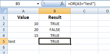
In the first example, I am using a single condition only in the OR function. For that, we have a value in the A2 cell that is used in the OR function. The B2 cell shows the returned value by OR.
Similarly, other A column cells are used for different result; all with single condition:
The formulas for different B cells are:
|
B2: =OR(A2>5) B3: =OR(A3<=10) B4: =OR(A4=15) B5: =OR(A5=«test») |
You can see the output in the above examples. Also, notice the usage of text in the OR function and the returned result.
Using multiple conditions example
For this example, I used two or more conditions in the OR function. To make it understand how it works, various combinations of True/False returned results are used as follows:
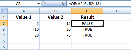
The formulas for C column (C2 to C4):
|
C2: =OR(A2>5, B2<15) C3: =OR(A3=-10,B3>20) C4: =OR(A4=15,B4=-5,A2>=10) |
You can see, the returned result is False for only that formula for which all conditions are False. That is the C2 cell’s formula. In that case, neither A2 is greater than 5 nor B2 is less than 15.
In other cases, even one condition is True, the OR function returned the True.
An example of using the OR with IF function
Just like AND function, we may use the OR in conjunction with the IF function. In that case, the OR acts as the logical test in the IF function.
An example below shows the usage of OR function with IF. For that, we have an Excel sheet that contains the records of “Number of Sales” and “Sale amount” by the Sales Persons.
A salesperson is eligible for the bonus only if the number of sales is greater than or equal to 50. Similarly, if the sales amount is greater than $10,000, he/she is eligible for the bonus even if the number of sales is less than 50.
See how IF/OR functions are used to get the results:
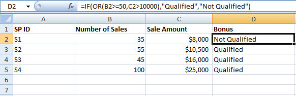
The formula used in the D2 cell to get the result for sales person 1:
|
=IF(OR(B2>=50,C2>10000),«Qualified»,«Not Qualified») |
To get the result for other salespersons, just replace the B2 and C2 cells by their respective cells.
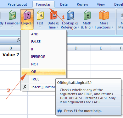
How to use ribbon for creating OR formula?
Rather than writing the formula in the formula bar yourself, you may also provide OR function arguments by accessing the menu in the ribbon.
To access the OR function:
Step 1:
Select a cell where you want to apply the formula and
Go to the “Formulas” in the ribbon
Step 2:
Locate the “Logical” group and click on the “OR” as shown below:
The “Function Arguments” popup comes up where you may enter up to 255 conditions that you want to test.
Enter the condition(s) as shown below:
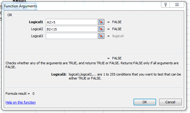
You can see the result as you are entering the conditions.
Excel AND + OR Functions: Full Guide (with IF Formulas)
The AND and OR functions returns True or False if certain conditions are met.
Combined with other functions, like IF, that enables multiple criteria logic in your formulas.
In this guide, I’ll walk you through all of this, step-by-step 👍🏼
If you want to tag along, download the sample workbook here.
We use the data in the following table to learn how to apply OR and AND function with the IF function in excel.

The OR function
The OR function is one of the most important logical functions in excel 😯
The OR function in Excel returns True if at least one of the criteria evaluates to true.
If all the arguments evaluate as False, then the OR function returns False.
The syntax of the OR function in Excel is OR(logical1, [logical2], …).
Assume that employees are eligible for an incentive if they achieve a value or volume target of 75% or more 🏆
Let’s try OR function for the above example.
- Enter an equal sign and select the OR function.
You will see below in the formula bar.
=OR(

- Supply the first logical value to evaluate as the first argument.
You can write logical values to test using logical operators.
In this case, we want to first test, whether the value target achievement is greater than or equal to 75%.
So, we can give the cell reference and write the condition >=75%.
Now the formula is,
=OR(B3>=75%

- Enter a comma and enter the 2nd logical value for the logical test.
Then, we enter the logical value for the volume target.
Now, the updated formula is;
=OR(B3>7=75%,C3>=75%

- Close the parentheses and press enter.
The below Excel formula evaluates arguments.
=OR(B3>7=75%,C3>=75%)
Then returns true if at least one of the value or volume target achievements is greater than or equal to 75%. If both value and volume target achievements are below 75%, the OR function returns False.

Pro Tip:
Now you have learned, the OR function returns True even when more than one condition evaluates to “True”.
Do you think you have to combine the OR function with the NOT function?
No. Excel has a simple solution 😜
You have to use the XOR function.
Apply the below XOR formula to the above example and see how the results are changing.
=XOR(B3>7=75%,C3>=75%)

You can see that Mary’s result is “False” as her achievements are not satisfying the one and only condition.
OR function IF formula example
Isn’t it boring to see only “True or false” values? 🥱
Don’t you like to get something other than True or False values? 👍
You just need to combine the OR function with the IF function in Excel.
Let’s say, we want the function to return “Eligible” if at least one of the value or volume target achievements is greater than or equal to 75%.
Also, return “Not eligible”, if both value and volume target achievements are less than 75%.
- Enter the equal sign and select the IF function.
Now, the formula bar will show;

- Enter the OR function that we have learned in the previous section.
The updated formula should be like this.
=IF(OR(B3>=75%,C3>=75%)

- Enter the specific value you want the function to return when the result of the logical test is True.
In this case, we want to get “Eligible”.
So, we enter the word eligible within quotes.
Now, the formula is;
=IF(OR(B3>=75%,C3>=75%),”Eligible”

If you want to enter text values for the arguments, you have to enter them within quotes. However, you don’t need to enter True or false values within quotes. Excel automatically evaluates arguments provided with true or false values.
- Enter the specific value you want the function to return when the result of the logical test is False.
In this case, we want to get “Not Eligible”.
Now, the updated formula is;
=IF(OR(B3>=75%,C3>=75%),”Eligible”,”Not Eligible”

- Close the parentheses and press “Enter”.

The AND function
AND function is another important logical function in excel.
This function returns true all of the multiple criteria are true.
Otherwise, the AND function returns False.
The syntax of the AND function in Excel is AND(logical1, [logical2], …).
Say that employees are entitled to an incentive if they achieve more than or equal to 75% for both the value target and volume target.
Let’s try AND function for the above example.
- Enter an equal sign and select the AND function.
You will see below in the formula bar.
=AND(

- Enter all logical values to test using logical operators.
So, you can enter the following formula.
=AND(B3>=75%,C3>=75%

- Close the parentheses and press “Enter”.

You can see that the AND function returns true only when both the value and volume target achievements exceed or are equal to 75% 🥳
However, there is limited usage of AND function if we do not combine it with other functions in Excel 🤔
Let’s see an example with a combination of the IF function and AND function.
AND function IF formula example
Let’s say, we want the function to return “Eligible”, only when both value and volume target achievements are more than or equal to 75%.
Otherwise, we want to get “Not eligible”
- Enter the equals sign and select the IF function.
Now, the formula bar will show;

- Enter the AND function that we have learned in the previous section.
The updated formula should be like this.
=IF(AND(B3>=75%,C3>=75%)

- Enter the specific value you want the function to return when the result of the logical test is True.
In this case, we want to get “Eligible”.
So, we enter the word eligible within quotes.
Now, the formula is;
=IF(AND(B3>=75%,C3>=75%),”Eligible”

- Enter the specific value you want the function to return when the result of the logical test is False.
In this case, we want to get “Not Eligible”.
Now, the updated formula is;
=IF(AND(B3>=75%,C3>=75%),”Eligible”,”Not Eligible”

- Close the parentheses and press “Enter”.

You can see that we get “Eligible” only when all of the multiple conditions are True. Otherwise, functions will return false 😍
Any empty cells in a logical function’s argument are ignored.

That’s it – Now what?
Well done 👏🏻
Now you know how to use the OR and AND functions in Excel.
Using the above examples, you have learned that OR and AND functions are more powerful when we combine them with other Excel functions 💪🏻
To learn more about other important functions such as IF, SUMIF, and VLOOKUP functions, all you need to do is enroll in my free 30-minute online Excel course.
Other resources
When you are using OR and AND functions, it is extremely important to use logical operators correctly ⚡
Read our article about logical operators, if you want to refresh your knowledge about them.
Also, Read our articles about the IF function, nested IF function, and SUMIF function and apply OR and AND functions more effectively 🥳
Frequently asked questions
You can enter 2 conditions or more for the logical test argument of the IF function using the following formulas.
If you want to satisfy,
- Both conditions – use the AND function.
- At least one condition – use the OR function
- Only one condition – use the XOR function.
Yes. We can use multiple logical functions with the IF function in Excel.
You can combine OR and AND functions to evaluate the arguments appropriately.
Kasper Langmann2023-02-23T11:04:48+00:00
Page load link
In this article, we will learn How to use the OR function in Excel.
What is the OR function used for ?
OR function is logical operator. Whenever we deal with multiple values at one time, we need to check whether we need to consider different things. If you need the return value True wherever any row can have this or that. For example matching multiple employee IDs. Using OR function you can provide as many criteria you like and if any one those criteria is True. The function returns TRUE.
OR Function in Excel
OR function only returns TRUE or FALSE.
Syntax:
=OR(logical1, [logical2], [logical3], …)
logical1 : First criteria
[logical2] :
[logical3]
Example :
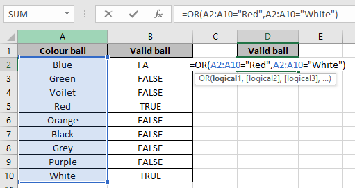
All of these might be confusing to understand. Let’s understand how to use the function using an example. Here we have some coloured balls and we need to test the condition to check whether the ball is valid or not.
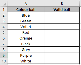
Use the formula in B2 cell.
Explanation:
Function checks either Red ball or White ball is valid for the match to be played.
So it checks the cell A2 for the same.
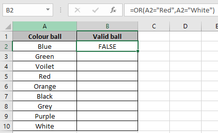
As it returns False means it doesn’t have either Red or White.
Use the Ctrl + D option to check the cells corresponding to it.
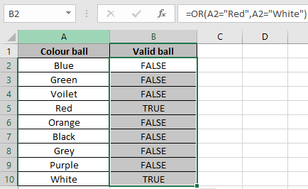
As we can see in the above snapshot it returns True for the cells having Red or White coloured ball.
You can apply it to check on the range of cells to test whether any of the cell returns True or not.
Use the formula
=OR(A2:A10=»Red»,A2:A10=»White»)
Note: Don’t forget to use Ctrl + shift + Enter to get the result. Curly brackets will be visible in the formula bar (fx) of the cell.
Use Ctrl + Shift + Enter to see the result
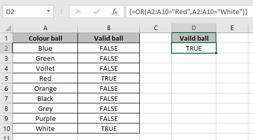
It returns True. It means that A2:A10 range cells have either White or Red ball.
You can check less than or greater than condition on numbers. OR function can also be used along with many function like IF, AND and many more.
IF with OR function
We have a list of months and need to know in which quarter it lay.
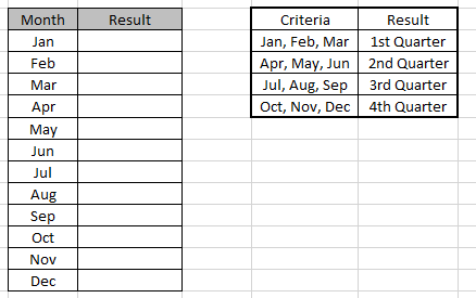
Use the formula to match the quarter of the months
Formula:
=IF(OR(A4=”Jan”,A4=”Feb”,A4=”Mar”),”1st Quarter”,IF(OR(A4=”Apr”,A4=”May”,A4=”Jun”),”2nd Quarter”,IF(OR(A4=”Jul”,A4=”Aug”,A4=”Sep”),”3rd Quarter”,IF(OR(A4=”Oct”,A4=”Nov”,A4=”Dec”),”4th Quarter”))))
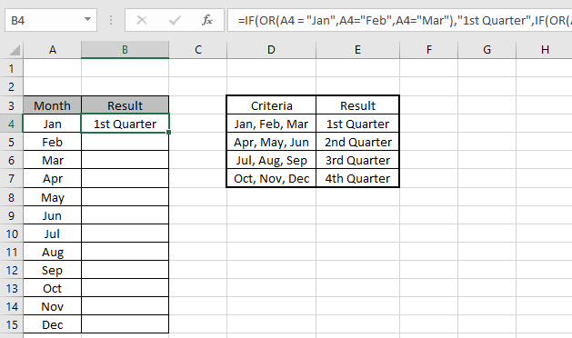
Copy the formula in other cells, select the cells taking the first cell where the formula is already applied, use shortcut key Ctrl +D
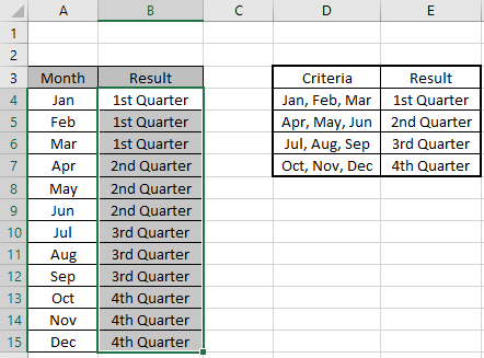
We got the result.
You can also use the SUMPRODUCT function if you are comfortable with it. How to use the SUMPRODUCT function in Excel
Here are all the observational notes using the OR function in Excel
Notes :
- Different criteria must be separated using comma ( , )
- Operations like equals to ( = ), less than equal to ( <= ), greater than ( > ) or not equals to ( <> ) can be performed within a formula applied, with numbers only.
Hope this article about How to use the OR function in Excel is explanatory. Find more articles on checking values and related Excel formulas here. If you liked our blogs, share it with your friends on Facebook. And also you can follow us on Twitter and Facebook. We would love to hear from you, do let us know how we can improve, complement or innovate our work and make it better for you. Write to us at info@exceltip.com.
Related Articles :
How to Count Cells That Contain This Or That in Excel in Excel :To cells that contain this or that, we can use the SUMPRODUCT function. Here’s how you do those calculations.
IF with OR function : Implementation of logic IF function with OR function to extract results having criteria in excel data.
IF with AND function : Implementation of logic IF function with AND function to extract results having criteria in Excel.
How to use nested IF function : nested IF function operates on data having multiple criteria. The use of repeated IF function is nested IF excel formula.
SUMIFS using AND-OR logic : Get the sum of numbers having multiple criteria applied using logic AND-OR excel function.
COUNTIFS With OR For Multiple Criteria : Count cells having multiple criteria match using the OR function. To put an OR logic in COUNTIFS function you will not need to use the OR function.
Using the IF with AND / OR Functions in Microsoft Excel : These logical functions are used to carry out multiple criteria calculations. With IF the OR and AND functions are used to include or exclude matches.
Popular Articles :
How to use the IF Function in Excel : The IF statement in Excel checks the condition and returns a specific value if the condition is TRUE or returns another specific value if FALSE.
How to use the VLOOKUP Function in Excel : This is one of the most used and popular functions of excel that is used to lookup value from different ranges and sheets.
How to use the SUMIF Function in Excel : This is another dashboard essential function. This helps you sum up values on specific conditions.
How to use the COUNTIF Function in Excel : Count values with conditions using this amazing function. You don’t need to filter your data to count specific values. Countif function is essential to prepare your dashboard.