
Excel for Microsoft 365 Excel for Microsoft 365 for Mac Excel for the web Excel 2021 Excel 2021 for Mac Excel 2019 Excel 2019 for Mac Excel 2016 Excel 2016 for Mac Excel 2013 Excel for iPad Excel for iPhone Excel for Android tablets Excel 2010 Excel 2007 Excel for Mac 2011 Excel for Android phones Excel Mobile More…Less
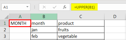
Unlike Microsoft Word, Microsoft Excel doesn’t have a Change Case button for changing capitalization. However, you can use the UPPER, LOWER, or PROPER functions to automatically change the case of existing text to uppercase, lowercase, or proper case. Functions are just built-in formulas that are designed to accomplish specific tasks—in this case, converting text case.
How to Change Case
In the example below, the PROPER function is used to convert the uppercase names in column A to proper case, which capitalizes only the first letter in each name.
-
First, insert a temporary column next to the column that contains the text you want to convert. In this case, we’ve added a new column (B) to the right of the Customer Name column.

In cell B2, type =PROPER(A2), then press Enter.
This formula converts the name in cell A2 from uppercase to proper case. To convert the text to lowercase, type =LOWER(A2) instead. Use =UPPER(A2) in cases where you need to convert text to uppercase, replacing A2 with the appropriate cell reference.
-
Now, fill down the formula in the new column. The quickest way to do this is by selecting cell B2, and then double-clicking the small black square that appears in the lower-right corner of the cell.
Tip: If your data is in an Excel table, a calculated column is automatically created with values filled down for you when you enter the formula.
-
At this point, the values in the new column (B) should be selected. Press CTRL+C to copy them to the Clipboard.
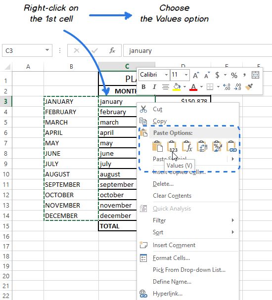
Right-click cell A2, click Paste, and then click Values. This step enables you to paste just the names and not the underlying formulas, which you don’t need to keep.
-
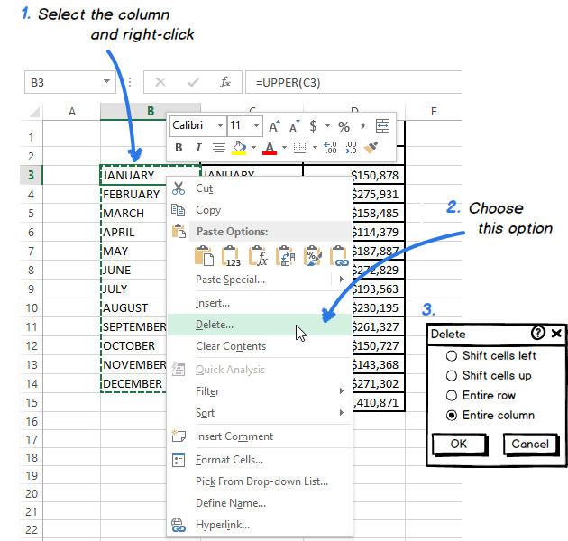
You can then delete column (B), since it is no longer needed.
Need more help?
You can always ask an expert in the Excel Tech Community or get support in the Answers community.
See Also
Use AutoFill and Flash Fill
Need more help?
Want more options?
Explore subscription benefits, browse training courses, learn how to secure your device, and more.
Communities help you ask and answer questions, give feedback, and hear from experts with rich knowledge.
Содержание
- Трансформация строчных символов в прописные
- Способ 1: функция ПРОПИСН
- Способ 2: применение макроса
- Вопросы и ответы

В некоторых ситуациях весь текст в документах Excel требуется писать в верхнем регистре, то есть, с заглавной буквы. Довольно часто, например, это нужно при подаче заявлений или деклараций в различные государственные органы. Чтобы написать текст большими буквами на клавиатуре существует кнопка Caps Lock. При её нажатии запускается режим, при котором все введенные буквы будут заглавными или, как говорят по-другому, прописными.
Но, что делать, если пользователь забыл переключиться в верхний регистр или узнал о том, что буквы нужно было сделать в тексте большими лишь после его написания? Неужели придется переписывать все заново? Не обязательно. В Экселе существует возможность решить данную проблему гораздо быстрее и проще. Давайте разберемся, как это сделать.
Читайте также: Как в Ворде сделать текст заглавными буквами
Трансформация строчных символов в прописные
Если в программе Word для преобразования букв в заглавные (прописные) достаточно выделить нужный текст, зажать кнопку SHIFT и дважды кликнуть по функциональной клавише F3, то в Excel так просто решить проблему не получится. Для того, чтобы преобразовать строчные буквы в заглавные, придется использовать специальную функцию, которая называется ПРОПИСН, или воспользоваться макросом.
Способ 1: функция ПРОПИСН
Сначала давайте рассмотрим работу оператора ПРОПИСН. Из названия сразу понятно, что его главной целью является преобразование букв в тексте в прописной формат. Функция ПРОПИСН относится к категории текстовых операторов Excel. Её синтаксис довольно прост и выглядит следующим образом:
=ПРОПИСН(текст)
Как видим, оператор имеет всего один аргумент – «Текст». Данный аргумент может являться текстовым выражением или, что чаще, ссылкой на ячейку, в которой содержится текст. Данный текст эта формула и преобразует в запись в верхнем регистре.
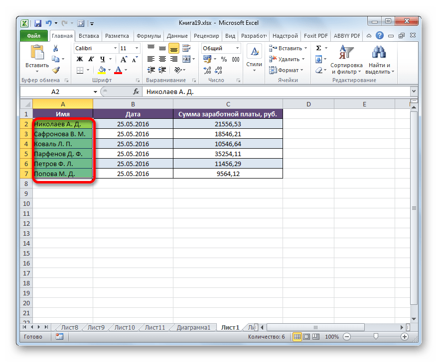
Теперь давайте на конкретном примере разберемся, как работает оператор ПРОПИСН. У нас имеется таблица с ФИО работников предприятия. Фамилия записана в обычном стиле, то есть, первая буква заглавная, а остальные строчные. Ставится задача все буквы сделать прописными (заглавными).
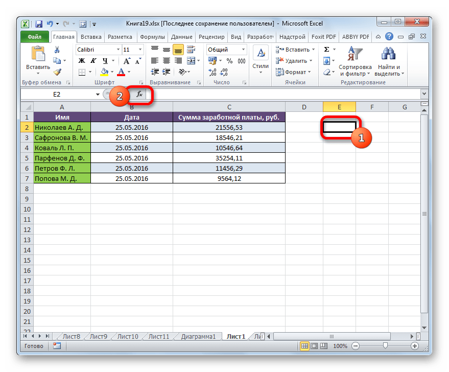
- Выделяем любую пустую ячейку на листе. Но более удобно, если она будет располагаться в параллельном столбце тому, в котором записаны фамилии. Далее щелкаем по кнопке «Вставить функцию», которая размещена слева от строки формул.
- Запускается окошко Мастера функций. Перемещаемся в категорию «Текстовые». Находим и выделяем наименование ПРОПИСН, а затем жмем на кнопку «OK».
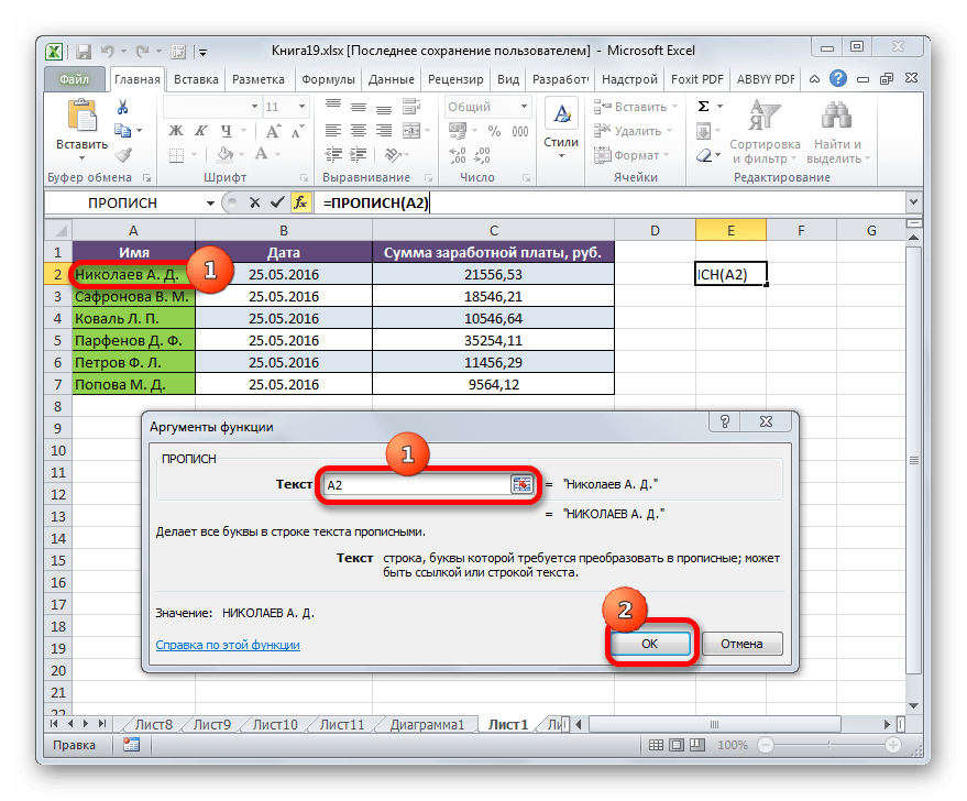
- Происходит активация окна аргументов оператора ПРОПИСН. Как видим, в этом окне всего одно поле, которое соответствует единственному аргументу функции – «Текст». Нам нужно в это поле ввести адрес первой ячейки в столбце с фамилиями работников. Это можно сделать вручную. Вбив с клавиатуры туда координаты. Существует также и второй вариант, который более удобен. Устанавливаем курсор в поле «Текст», а потом кликаем по той ячейке таблицы, в которой размещена первая фамилия работника. Как видим, адрес после этого отображается в поле. Теперь нам остается сделать последний штрих в данном окне – нажать на кнопку «OK».
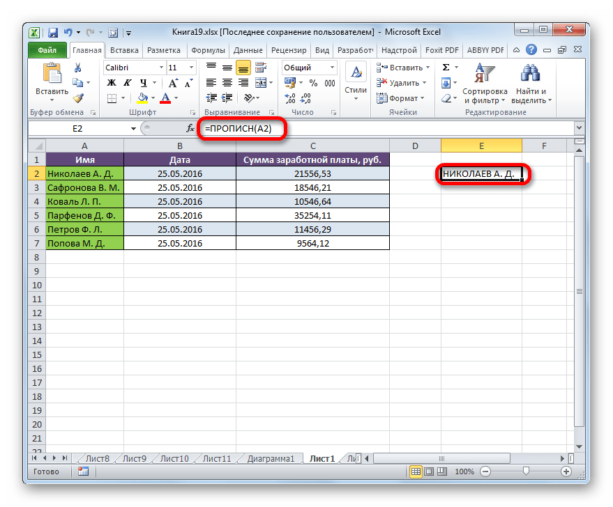
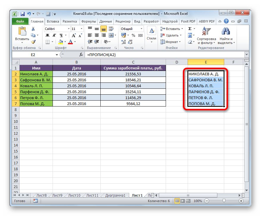
- После этого действия содержимое первой ячейки столбца с фамилиями выводится в предварительно выделенный элемент, в котором содержится формула ПРОПИСН. Но, как видим, все отображаемые в данной ячейке слова состоят исключительно из заглавных букв.
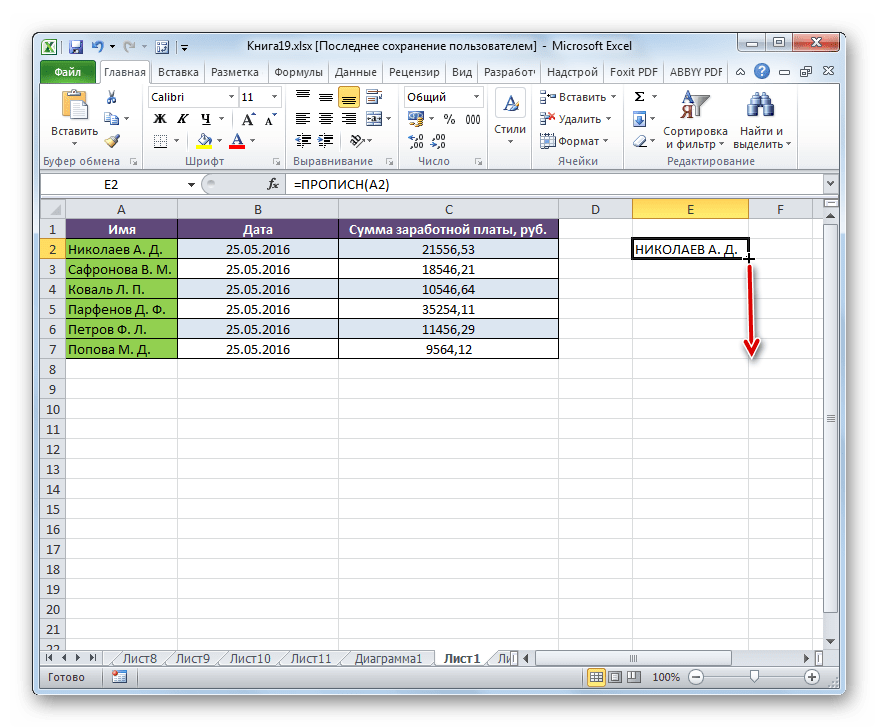
- Теперь нам нужно произвести преобразование и для всех других ячеек столбца с фамилиями работников. Естественно, мы не будем для каждого сотрудника применять отдельную формулу, а просто скопируем уже существующую при помощи маркера заполнения. Для этого ставим курсор в нижний правый угол элемента листа, в котором содержится формула. После этого курсор должен преобразоваться в маркер заполнения, который выглядит как небольшой крестик. Производим зажим левой кнопки мыши и тянем маркер заполнения на количество ячеек равное их числу в столбце с фамилиями сотрудников предприятия.
- Как видим, после указанного действия все фамилии были выведены в диапазон копирования и при этом они состоят исключительно из заглавных букв.
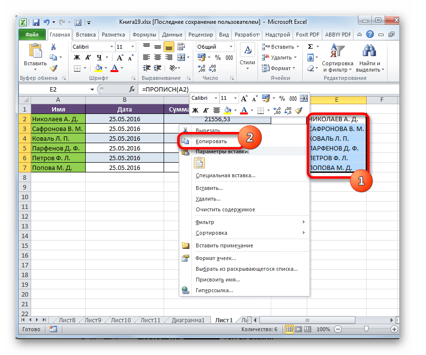
- Но теперь все значения в нужном нам регистре расположены за пределами таблицы. Нам же нужно вставить их в таблицу. Для этого выделяем все ячейки, которые заполнены формулами ПРОПИСН. После этого кликаем по выделению правой кнопкой мыши. В открывшемся контекстном меню выбираем пункт «Копировать».
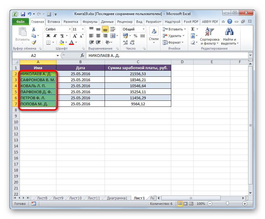
- После этого выделяем столбец с ФИО сотрудников предприятия в таблице. Кликаем по выделенному столбцу правой кнопкой мыши. Запускается контекстное меню. В блоке «Параметры вставки» выбираем пиктограмму «Значения», которая отображена в виде квадрата, содержащего цифры.
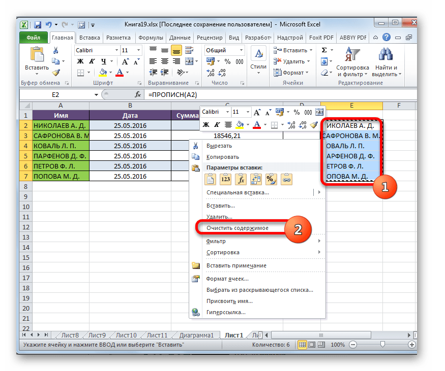
- После этого действия, как видим, преобразованный вариант написания фамилий заглавными буквами будет вставлен в исходную таблицу. Теперь можно удалить диапазон, заполненный формулами, так как он нам больше не нужен. Выделяем его и кликаем правой кнопкой мыши. В контекстном меню выбираем пункт «Очистить содержимое».


После этого работу над таблицей по преобразованию букв в фамилиях сотрудников в прописные можно считать завершенной.
Урок: Мастер функций в Экселе
Способ 2: применение макроса
Решить поставленную задачу по преобразованию строчных букв в прописные в Excel можно также при помощи макроса. Но прежде, если в вашей версии программы не включена работа с макросами, нужно активировать эту функцию.
- После того, как вы активировали работу макросов, выделяем диапазон, в котором нужно трансформировать буквы в верхний регистр. Затем набираем сочетание клавиш Alt+F11.
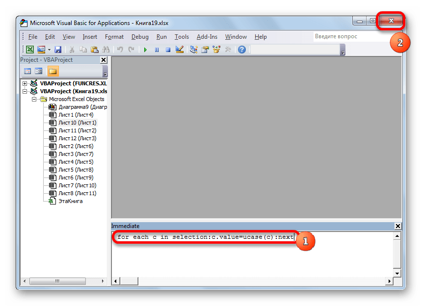
- Запускается окно Microsoft Visual Basic. Это, собственно, редактор макросов. Набираем комбинацию Ctrl+G. Как видим, после этого курсор перемещается в нижнее поле.
- Вводим в это поле следующий код:
for each c in selection:c.value=ucase(c):nextЗатем жмем на клавишу ENTER и закрываем окно Visual Basic стандартным способом, то есть, нажав на кнопку закрытия в виде крестика в его правом верхнем углу.
- Как видим, после выполнения вышеуказанных манипуляций, данные в выделенном диапазоне преобразованы. Теперь они полностью состоят из прописных букв.


Урок: Как создать макрос в Excel
Для того, чтобы сравнительно быстро преобразовать все буквы в тексте из строчных в прописные, а не терять время на его ручное введение заново с клавиатуры, в Excel существует два способа. Первый из них предусматривает использование функции ПРОПИСН. Второй вариант ещё проще и быстрее. Но он основывается на работе макросов, поэтому этот инструмент должен быть активирован в вашем экземпляре программы. Но включение макросов – это создание дополнительной точки уязвимости операционной системы для злоумышленников. Так что каждый пользователь решает сам, какой из указанных способов ему лучше применить.
Еще статьи по данной теме:
Помогла ли Вам статья?
You’ve probably come across this situation before.
You have a list of names and it’s all lower case letter. You need to fix them so they are all properly capitalized.
With hundreds of names in your list, it’s going to be a pain to go through and edit first and last names.
Thankfully, there are some easy ways to change the case of any text data in Excel. We can change text to lower case, upper case or proper case where each word is capitalized.
In this post, we’re going to look at using Excel functions, flash fill, power query, DAX and power pivot to change the case of our text data.
Video Tutorial
Using Excel Formulas To Change Text Case
The first option we’re going to look at is regular Excel functions. These are the functions we can use in any worksheet in Excel.
There’s a whole category of Excel functions to deal with text, and these three will help us to change the text case.
LOWER Excel Worksheet Function
=LOWER(Text)The LOWER function takes one argument which is the bit of Text we want to change into lower case letters. The function will evaluate to text that is all lower case.
UPPER Excel Worksheet Function
=UPPER(Text)The UPPER function takes one argument which is the bit of Text we want to change into upper case letters. The function will evaluate to text that is all upper case.
PROPER Excel Worksheet Function
=PROPER(Text)The PROPER function takes one argument which is the bit of Text we want to change into proper case. The function will evaluate to text that is all proper case where each word starts with a capital letter and is followed by lower case letters.
Copy And Paste Formulas As Values
After using the Excel formulas to change the case of our text, we may want to convert these to values.
This can be done by copying the range of formulas and pasting them as values with the paste special command.
Press Ctrl + C to copy the range of cells ➜ press Ctrl + Alt + V to paste special ➜ choose Values from the paste options.
Using Flash Fill To Change Text Case
Flash fill is a tool in Excel that helps with simple data transformations. We only need to provide a couple examples of the results we want, and flash fill will fill in the rest.
Flash fill can only be used directly to the right of the data we’re trying to transform. We need to type out a couple of examples of the results we want. When Excel has enough examples to figure out the pattern, it will show the suggested data in a light grey font. We can accept this suggested filled data by pressing Enter.
We can also access flash fill from the ribbon. Enter the example data ➜ highlight both the examples and cells that need to be filled ➜ go to the Data tab ➜ press the Flash Fill command found in the Data Tools section.
We can also use the keyboard shortcut Ctrl + E for flash fill.
Flash fill will work for many types of simple data transformations including changing text between lower case, upper case and proper case.
Using Power Query To Change Text Case
Power query is all about data transformation, so it’s sure there is a way to change the case of text in this tool.
With power query we can transform the case into lower, upper and proper case.
Select the data we want to transform ➜ go to the Data tab ➜ select From Table/Range. This will open up the power query editor where we can apply our text case transformations.
Text.Lower Power Query Function
Select the column containing the data we want to transform ➜ go to the Add Column tab ➜ select Format ➜ select lowercase from the menu.
= Table.AddColumn(#"Changed Type", "lowercase", each Text.Lower([Name]), type text)This will create a new column with all text converted to lower case letters using the Text.Lower power query function.
Text.Upper Power Query Function
Select the column containing the data we want to transform ➜ go to the Add Column tab ➜ select Format ➜ select UPPERCASE from the menu.
= Table.AddColumn(#"Changed Type", "UPPERCASE", each Text.Upper([Name]), type text)This will create a new column with all text converted to upper case letters using the Text.Upper power query function.
Text.Proper Power Query Function
Select the column containing the data we want to transform ➜ go to the Add Column tab ➜ select Format ➜ select Capitalize Each Word from the menu.
= Table.AddColumn(#"Changed Type", "Capitalize Each Word", each Text.Proper([Name]), type text)This will create a new column with all text converted to proper case lettering, where each word is capitalized, using the Text.Proper power query function.
Using DAX Formulas To Change Text Case
When we think of pivot tables, we generally think of summarizing numeric data. But pivot tables can also summarize text data when we use the data model and DAX formulas. There are even DAX formula to change text case before we summarize it!
First, we need to create a pivot table with our text data. Select the data to be converted ➜ go to the Insert tab ➜ select PivotTable from the tables section.
In the Create PivotTable dialog box menu, check the option to Add this data to the Data Model. This will allow us to use the necessary DAX formula to transform our text case.
Creating a DAX formula in our pivot table can be done by adding a measure. Right click on the table in the PivotTable Fields window and select Add Measure from the menu.
This will open up the Measure dialog box, where we can create our DAX formulas.
LOWER DAX Function
=CONCATENATEX( ChangeCase, LOWER( ChangeCase[Mixed Case] ), ", ")We can enter the above formula into the Measure editor. Just like the Excel worksheet functions, there is a DAX function to convert text to lower case.
However, in order for the expression to be a valid measure, it will need to be wrapped in a text aggregating function like CONCATENATEX. This is because measures need to evaluate to a single value and the LOWER DAX function does not do this on it’s own. The CONCATENATEX function will aggregate the results of the LOWER function into a single value.
We can then add the original column of text into the Rows and the new Lower Case measure into the Values area of the pivot table to produce our transformed text values.
Notice the grand total of the pivot table contains all the names in lower case text separated by a comma and space character. We can hide this part by going to the Table Tools Design tab ➜ Grand Totals ➜ selecting Off for Rows and Columns.
UPPER DAX Function
=CONCATENATEX( ChangeCase, UPPER( ChangeCase[Mixed Case] ), ", ")Similarily, we can enter the above formula into the Measure editor to create our upper case DAX formula. Just like the Excel worksheet functions, there is a DAX function to convert text to upper case.
Creating the pivot table to display the upper case text is the same process as with the lower case measure.
Missing PROPER DAX Function
We might try and create a similar DAX formula to create proper case text. But it turns out there is no function in DAX equivalent to the PROPER worksheet function.
Using Power Pivot Row Level Formulas To Change Text Case
This method will also use pivot tables and the Data Model, but instead of DAX formulas we can create row level calculations using the Power Pivot add-in.
Power pivot formulas can be used to add new calculated columns in our data. Calculations in these columns happen for each row of data similar to our regular Excel worksheet functions.
Not every version of Excel has power pivot available and you will need to enable the add-in before you can use it. To enable the power pivot add-in, go to the File tab ➜ Options ➜ go to the Add-ins tab ➜ Manage COM Add-ins ➜ press Go ➜ check the box for Microsoft Power Pivot for Excel.
We will need to load our data into the data model. Select the data ➜ go to the Power Pivot tab ➜ press the Add to Data Model command.
This is the same data model as creating a pivot table and using the Add this data to the Data Model checkbox option. So if our data is already in the data model we can use the Manage data model option to create our power pivot calculations.
LOWER Power Pivot Function
=LOWER(ChangeCase[Mixed Case])Adding a new calculated column into the data model is easy. Select an empty cell in the column labelled Add Column then type out the above formula into the formula bar. You can even create references in the formula to other columns by clicking on them with the mouse cursor.
Press Enter to accept the new formula.
The formula will appear in each cell of the new column regardless of which cell was selected. This is because each row must use the same calculation within a calculated column.
We can also rename our new column by double clicking on the column heading. Then we can close the power pivot window to use our new calculated column.
When we create a new pivot table with the data model, we will see the calculated column as a new available field in our table and we can add it into the Rows area of the pivot table. This will list out all the names in our data and they will all be lower case text.
UPPER Power Pivot Function
=UPPER(ChangeCase[Mixed Case])We can do the same thing to create a calculated column that converts the text to upper case by adding a new calculated column with the above formula.
Again, we can then use this as a new field in any pivot table created from the data model.
Missing PROPER Power Pivot Function
Unfortunately, there is no power pivot function to convert text to proper case. So just like DAX, we won’t be able to do this in a similar fashion to the lower case and upper case power pivot methods.
Conclusions
There are many ways to change the case of any text data between lower, upper and proper case.
- Excel Formulas are quick, easy and will dynamically update if the inputs ever change.
- Flash fill is great for one-off transformations where you need to quickly fix some text and don’t need to update or change the data after.
- Power query is perfect for fixing data that will be imported regularly into Excel from an outside source.
- DAX and power pivot are can be used for fixing text to display within a pivot table.
Each option has different strengths and weaknesses so it’s best to become familiar will all methods so you can choose the one that will best suit your needs.
About the Author
John is a Microsoft MVP and qualified actuary with over 15 years of experience. He has worked in a variety of industries, including insurance, ad tech, and most recently Power Platform consulting. He is a keen problem solver and has a passion for using technology to make businesses more efficient.
Содержание
- Change the case of text
- How to Change Case
- Need more help?
- Uppercase in Excel
- How to Change Lowercase to Uppercase in excel? (10 Easy Steps)
- Advantages
- Disadvantages
- Things to Remember
- Recommended Articles
- Change the case of text
- How to Change Case
- Need more help?
- 4 ways for changing case in Excel
- Excel functions for changing text case
- Enter an Excel formula
- Copy a formula down a column
- Remove a helper column
- Use Microsoft Word to change case in Excel
- Converting text case with a VBA macro
- Quickly change case with the Cell Cleaner add-in
- Video: how to change case in Excel
Change the case of text
Unlike Microsoft Word, Microsoft Excel doesn’t have a Change Case button for changing capitalization. However, you can use the UPPER, LOWER, or PROPER functions to automatically change the case of existing text to uppercase, lowercase, or proper case. Functions are just built-in formulas that are designed to accomplish specific tasks—in this case, converting text case.
How to Change Case
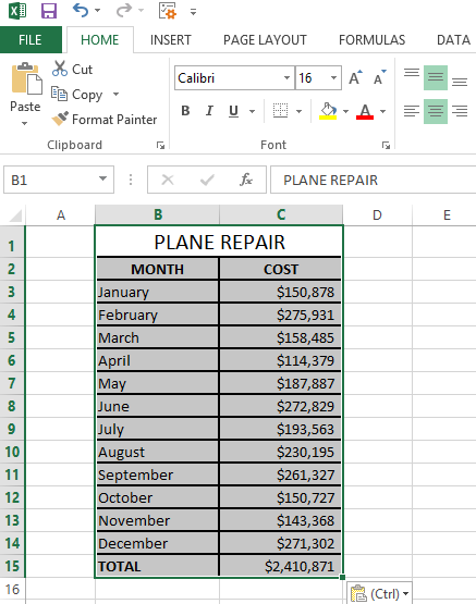
In the example below, the PROPER function is used to convert the uppercase names in column A to proper case, which capitalizes only the first letter in each name.
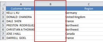
First, insert a temporary column next to the column that contains the text you want to convert. In this case, we’ve added a new column (B) to the right of the Customer Name column.
In cell B2, type =PROPER(A2), then press Enter.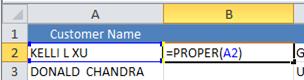
This formula converts the name in cell A2 from uppercase to proper case. To convert the text to lowercase, type =LOWER(A2) instead. Use =UPPER(A2) in cases where you need to convert text to uppercase, replacing A2 with the appropriate cell reference.
Now, fill down the formula in the new column. The quickest way to do this is by selecting cell B2, and then double-clicking the small black square that appears in the lower-right corner of the cell.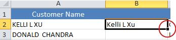
Tip: If your data is in an Excel table, a calculated column is automatically created with values filled down for you when you enter the formula.
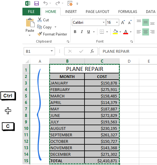
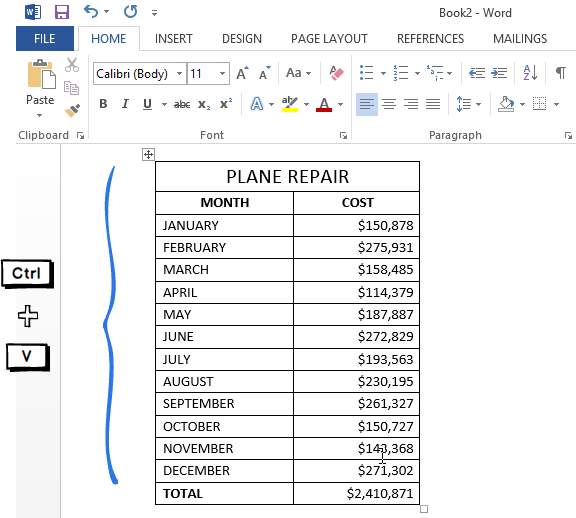
At this point, the values in the new column (B) should be selected. Press CTRL+C to copy them to the Clipboard.
Right-click cell A2, click Paste, and then click Values. This step enables you to paste just the names and not the underlying formulas, which you don’t need to keep.
You can then delete column (B), since it is no longer needed.
Need more help?
You can always ask an expert in the Excel Tech Community or get support in the Answers community.
Источник
Uppercase in Excel


How to Change Lowercase to Uppercase in excel? (10 Easy Steps)
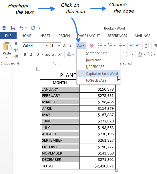
- Select the text data you want to convert in the upper case in Excel. You can choose at least one text cell to convert it.
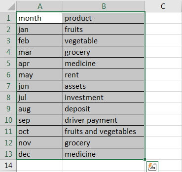
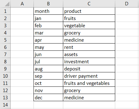
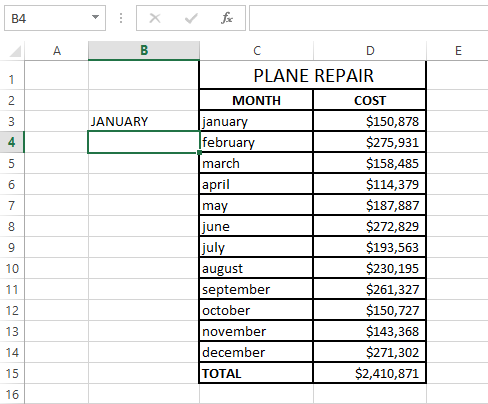
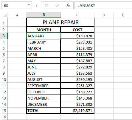
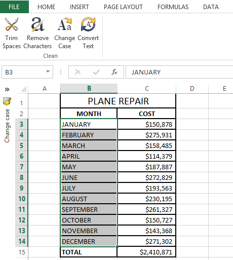
Insert the tab on the left side of the column (left to the “month” column) and use the adjacent column for data in the right column:
Enter the formula in both columns to change the text cases: =UPPER(text). This Excel formula is used where you want the text in uppercase only.
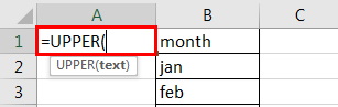
Use cell number in place of text in a column, which means that for which text you want the upper case.

Press the “Enter” key. You will get the B2 cell text in the upper case. It means that you have correctly made use of your formula.
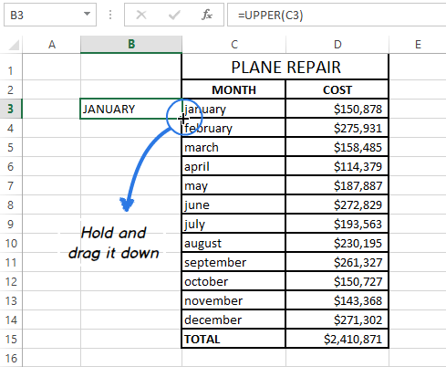
Drag the formula in all the rows. You will get the result with all the text versions in upper case only or copy the formula from the first cell to all the cells in a column.

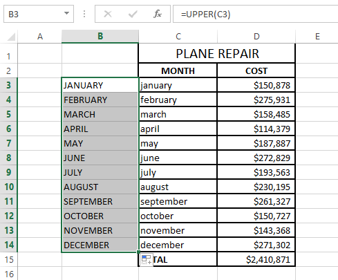
Once the data is in uppercase, copy it and paste it into the original column to remove the duplicate column you created while using the formula.
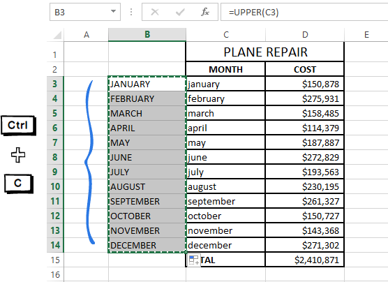
Select the column in which you have entered the formula and copy the column of the data.

Right-click the data and click on the “Values” icon under “Paste Options” in the dialog box menu.
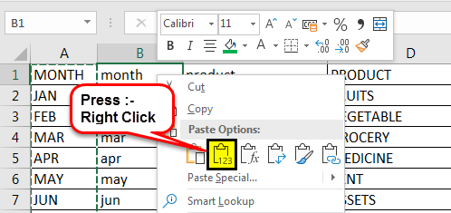
Paste the value in the original column. Then, delete the duplicate column in which you had to enter the formula to change the text case.
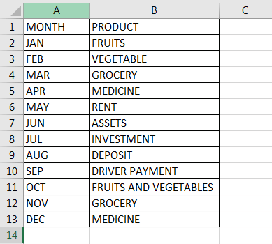
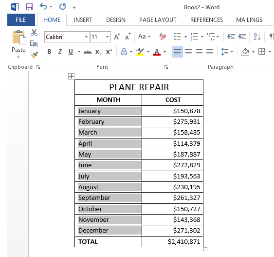
Now, you will see the values with all uppercase text in your data.
Table of contents
Advantages
- Uppercase in Excel is a very simple formula to use.
- It is worked in formulas that are intended to achieve explicit tasks.
- It does not affect the other data in the Excel workbook.
- It is easy using this function in huge data as well.
- Uppercase in Excel is very beneficial when you use the name of the person in your Excel workbooks.
- Using the Excel uppercase function in the workbook helps organize and make the data presentable.
- It helps to give an upper-case version of a given text in the Excel sheet if you use the upper-case formula punctuation, and numerical values are not affected.
Disadvantages
- The Excel uppercase function is not built-in in the Excel ribbon toolbar.
- We must copy and paste the data from one column to another to use this function.
- There is no shortcut key in Excel to use this function.
Things to Remember
- When copying the formula cells, we must always paste it in value format only. Otherwise, all the data will be mismatched, giving the wrong result.
- We must always add the temporary or duplicate column in your sheet to use this formula because it will help to paste the values in the original column.
- Do not forget to delete the duplicate column from the data.
- There is no shortcut key to use this function in the Excel workbook.
- While inserting the duplicate column, we have two options. First, we can delete or hide the column from the Excel workbook.
- When we have imported some text data or copied the data in the Excel worksheet, occasionally, the words have incorrect capitalization or case. E.g., all the text cases are in lower case, which shows that data is not in the correct case. Therefore, it results in a bad presentation of the data.
Recommended Articles
This article has been a guide to Uppercase in Excel. Here, we discuss converting lowercase text to uppercase in Excel, examples, and a downloadable Excel template. You may learn more about Excel from the following articles: –
Источник
Change the case of text
Unlike Microsoft Word, Microsoft Excel doesn’t have a Change Case button for changing capitalization. However, you can use the UPPER, LOWER, or PROPER functions to automatically change the case of existing text to uppercase, lowercase, or proper case. Functions are just built-in formulas that are designed to accomplish specific tasks—in this case, converting text case.
How to Change Case
In the example below, the PROPER function is used to convert the uppercase names in column A to proper case, which capitalizes only the first letter in each name.
First, insert a temporary column next to the column that contains the text you want to convert. In this case, we’ve added a new column (B) to the right of the Customer Name column.
In cell B2, type =PROPER(A2), then press Enter.
This formula converts the name in cell A2 from uppercase to proper case. To convert the text to lowercase, type =LOWER(A2) instead. Use =UPPER(A2) in cases where you need to convert text to uppercase, replacing A2 with the appropriate cell reference.
Now, fill down the formula in the new column. The quickest way to do this is by selecting cell B2, and then double-clicking the small black square that appears in the lower-right corner of the cell.
Tip: If your data is in an Excel table, a calculated column is automatically created with values filled down for you when you enter the formula.
At this point, the values in the new column (B) should be selected. Press CTRL+C to copy them to the Clipboard.
Right-click cell A2, click Paste, and then click Values. This step enables you to paste just the names and not the underlying formulas, which you don’t need to keep.
You can then delete column (B), since it is no longer needed.
Need more help?
You can always ask an expert in the Excel Tech Community or get support in the Answers community.
Источник
4 ways for changing case in Excel
 by Ekaterina Bespalaya, updated on November 24, 2022
In this article I’d like to tell you about different ways to change Excel uppercase to lowercase or proper case. You’ll learn how to perform these tasks with the help of Excel lower/upper functions, VBA macros, Microsoft Word, and an easy-to-use add-in by Ablebits.
The problem is that Excel doesn’t have a special option for changing text case in worksheets. I don’t know why Microsoft provided Word with such a powerful feature and didn’t add it to Excel. It would really make spreadsheets tasks easier for many users. But you shouldn’t rush into retyping all text data in your table. Fortunately, there are some good tricks to convert the text values in cells to uppercase, proper or lowercase. Let me share them with you.
Excel functions for changing text case
Microsoft Excel has three special functions that you can use to change the case of text. They are UPPER, LOWER and PROPER. The function allows you to convert all lowercase letters in a text string to uppercase. The function helps to exclude capital letters from text. The function makes the first letter of each word capitalized and leaves the other letters lowercase (Proper Case).
All three of these options work on the same principle, so I’ll show you how to use one of them. Let’s take the Excel uppercase function as an example.
Enter an Excel formula
- Insert a new (helper) column next to the one that contains the text you want to convert.
Note: This step is optional. If your table is not large, you can just use any adjacent blank column.
Your formula should look like this =UPPER(C3) , where C3 is the cell in the original column that has the text for conversion.
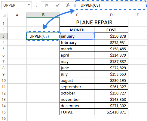
As you can see in the screenshot above, cell B3 contains the uppercase version of the text from cell C3.
Copy a formula down a column
Now you need to copy the formula to other cells in the helper column.
- Select the cell that includes the formula.
- Move your mouse cursor to the small square (fill handle) in the lower-right corner of the selected cell until you see a small cross.
Note: If you need to fill the new column down to the end of the table, you can skip steps 5-7 and just double-click on the fill handle.
Remove a helper column
So you have two columns with the same text data, but in different case. I suppose you’d like to leave only the correct one. Let’s copy the values from the helper column and then get rid of it.
- Highlight the cells that contain the formula and press Ctrl + C to copy them.
Since you need only the text values, pick this option to avoid formula errors later.
This theory might look very complicated to you. Take it easy and try to go through all these steps yourself. You’ll see that changing case with the use of Excel functions is not difficult at all.
Use Microsoft Word to change case in Excel
If you don’t want to mess with formulas in Excel, you can use a special command for changing text case in Word. Feel free to discover how this method works.
- Select the range where you want to change case in Excel.
- Press Ctrl + C or right-click on the selection and choose the Copy option from the context menu.
Now you’ve got your Excel table in Word.
Note: You can also select your text and press Shift + F3 until the style you want is applied. Using the keyboard shortcut you can choose only upper, lower or sentence case.
Now you have your table with the text case converted in Word. Just copy and paste it back to Excel.
Converting text case with a VBA macro
You can also use a VBA macro for changing case in Excel. Don’t worry if your knowledge of VBA leaves much to be desired. A while ago I didn’t know much about it as well, but now I can share three simple macros that make Excel convert text to uppercase, proper or lowercase.
I won’t labor the point and tell you how to insert and run VBA code in Excel because it was well described in one of our previous blog posts. I just want to show the macros that you can copy and paste into the code Module.
If you want to convert text to uppercase, you can use the following Excel VBA macro:
To apply Excel lowercase to your data, insert the code shown below into the Module window.
Pick the following macro if you want to convert your text values to proper / title case.
Quickly change case with the Cell Cleaner add-in
Looking at the three methods described above you might still think that there is no easy way to change case in Excel. Let’s see what the Cell Cleaner add-in can do to solve the problem. Probably, you’ll change your mind afterwards and this method will work best for you.
- Download the add-in and install it on your computer.
After the installation the new Ablebits Data tab appears in Excel.
The Change case pane displays to the left of your worksheet.
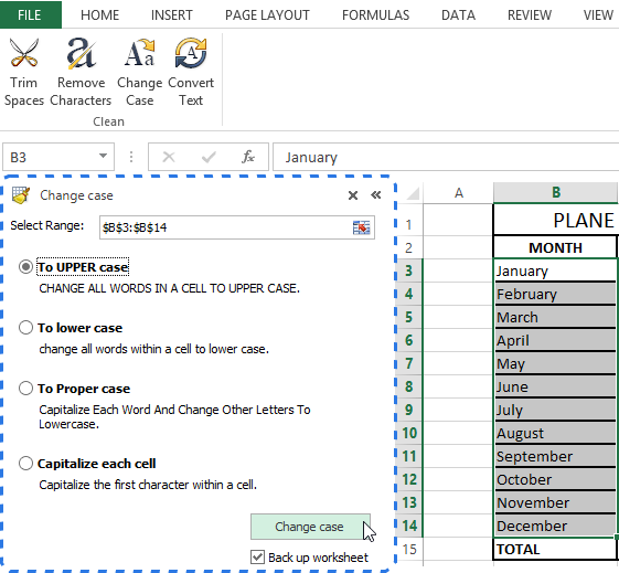
Note: If you want to keep the original version of your table, check the Back up worksheet box.
With Cell Cleaner for Excel the changing case routine seems to be much easier, doesn’t it?
Besides changing text case Cell Cleaner can help you to convert numbers in the text format to the number format, delete unwanted characters and excess spaces in your Excel table. Download the free 30-day trial version and check out how useful the add-in can be for you.
Video: how to change case in Excel
I hope now that you know nice tricks for changing case in Excel this task will never be a problem. Excel functions, Microsoft Word, VBA macros or Ablebits add-in are always there for you. You have a little left to do — just choose the tool that will work best for you.
Источник
![]()
Download Article
![]()
Download Article
When you’re working with improperly-capitalized data in Microsoft Excel, there’s no need to make manual corrections! Excel comes with two text-specific functions that can really be helpful when your data is in the wrong case. To make all characters appear in uppercase letters, you can use a simple function called UPPERCASE to convert one or more cells at a time. If you need your text to be in proper capitalization (first letter of each name or word is capitalized while the rest is lowercase), you can use the PROPER function the same way you’d use UPPERCASE. This wikiHow teaches you how to use the UPPERCASE and PROPER functions to capitalize your Excel data.
Steps
-
1
Type a series of text in a column. For example, you could enter a list of names, artists, food items—anything. The text you enter can be in any case, as the UPPERCASE or PROPER function will correct it later.[1]
-
2
Insert a column to the right of your data. If there’s already a blank column next to the column that contains your data, you can skip this step. Otherwise, right-click the column letter above your data column and select Insert.
- You can always remove this column later, so don’t worry if it messes up the rest of your spreadsheet right now.
Advertisement
-
3
Click the first cell in your new column. This is the cell to the right of the first cell you want to capitalize.
-
4
Click fx. This is the function button just above your data. The Insert Function window will expand.
-
5
Select the Text category from the menu. This displays Excel functions that pertain to handling text.
-
6
Select UPPER from the list. This function converts all letters to uppercase.
- If you’d rather just capitalize the first character of each part of a name (or the first character of each word, if you’re working with words), select PROPER instead.
- You could also use the LOWER function to convert all characters to lowercase.
-
7
Click OK. Now you’ll see «UPPER()» appear in the cell you clicked earlier. The Function Arguments window will also appear.
-
8
Highlight the cells you want to make uppercase. If you want to make everything in the column uppercase, just click the column letter above your data. A dotted line will surround the selected cells, and you’ll also see the range appear in the Function Arguments window.
- If you’re using PROPER, select all of the cells you want to make proper case—the steps are the same no matter which function you’re using.
-
9
Click OK. Now you’ll see the uppercase version of the first cell in your data appear at the first cell of your new column.
-
10
Double-click the bottom-right corner of the cell that contains your formula. This is the cell at the top of the column you inserted. Once you double-click the dot at the bottom of this cell, the formula will propagate to the remaining cells in the column, displaying the uppercase versions of your original column data.
- If you have trouble double-clicking that bottom-right corner, you can also drag that corner all the way down the column until you’ve reached the end of your data.
-
11
Copy the contents of your new column. For example, if your new column (the one that contains the now-uppercase versions of your original data) is column B, you’ll right-click the B above the column and select Copy.
-
12
Paste the values of the copied column over your original data. You’ll need to use a feature called Paste Values, which is different than traditional pasting. This option will replace your original data with just the uppercase versions of each entry (not the formulas). Here’s how to do it:
- Right-click the first cell in your original data. For example, if you started typing names or words into A1, you’d right-click A1.
- The Paste Values option might be in a different place, depending on your version of Excel. If you see a Paste Special menu, click that, select Values, and then click OK.
- If you see an icon with a clipboard that says «123,» click that to paste the values.
- If you see a Paste menu, select that and click Values.
-
13
Delete the column you inserted. Now that you’ve pasted the uppercase versions of your original data over that data, you can delete the formula column without harm. To do so, right-click the letter above the column and click Delete.


Advertisement

Add New Question
-
Question
Can I change to uppercase for an entire working sheet at one time?

Yes, you can do this by selecting the entire sheet then specifying you want it to be uppercase.
-
Question
How do I do uppercase when putting in a password?
You can’t use caps lock on some operating systems; try using the uppercase button
Ask a Question
200 characters left
Include your email address to get a message when this question is answered.
Submit
Advertisement
Thanks for submitting a tip for review!
About This Article
Article SummaryX
You can use the «UPPER» function in Microsoft Excel to transform lower-case letters to capitals. Start by inserting a blank column to the right of the column that contains your data. Click the first blank cell of the new column. Then, click the formula bar at the top of your worksheet—it’s the typing area that has an «fx» on its left side. Type an equal (=) sign, followed by the word «UPPER» in all capital letters. To tell the «UPPER» function which data to convert, click the first cell in your original data column. Press the Enter or Return key on your keyboard to apply the formula. The first cell of your original data column is now converted to uppercase letters. To apply this change to the entire column, click the cell containing the uppercase letters to select it. Then, drag the small square at the bottom-right corner of the cell down to the final row.
Did this summary help you?
Thanks to all authors for creating a page that has been read 1,463,548 times.