
Add or remove items from a drop-down list
Excel for Microsoft 365 Excel for Microsoft 365 for Mac Excel for the web Excel 2021 Excel 2021 for Mac Excel 2019 Excel 2019 for Mac Excel 2016 Excel 2016 for Mac Excel 2013 Excel 2010 Excel 2007 More…Less
After you create a drop-down list, you might want to add more items or delete items. In this article, we’ll show you how to do that depending on how the list was created.
Edit a drop-down list that’s based on an Excel Table
If you set up your list source as an Excel table, then all you need to do is add or remove items from the list, and Excel will automatically update any associated drop-downs for you.
-
To add an item, go to the end of the list and type the new item.
-
To remove an item, press Delete.
Tip: If the item you want to delete is somewhere in the middle of your list, right-click its cell, click Delete, and then click OK to shift the cells up.
-
Select the worksheet that has the named range for your drop-down list.
-
Do any of the following:
-
To add an item, go to the end of the list and type the new item.
-
To remove an item, press Delete.
Tip: If the item you want to delete is somewhere in the middle of your list, right-click its cell, click Delete, and then click OK to shift the cells up.
-
-
Go to Formulas > Name Manager.
-
In the Name Manager box, click the named range you want to update.

-
Click in the Refers to box, and then on your worksheet select all of the cells that contain the entries for your drop-down list.
-
Click Close, and then click Yes to save your changes.
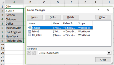
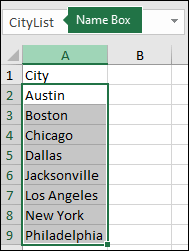
Tip: If you don’t know what a named range is named, you can select the range and look for its name in the Name Box. To locate a named range, see Find named ranges.
-
Select the worksheet that has the data for your drop-down list.
-
Do any of the following:
-
To add an item, go to the end of the list and type the new item.
-
To remove an item, click Delete.
Tip: If the item you want to delete is somewhere in the middle of your list, right-click its cell, click Delete, and then click OK to shift the cells up.
-
-
On the worksheet where you applied the drop-down list, select a cell that has the drop-down list.
-
Go to Data > Data Validation.
-
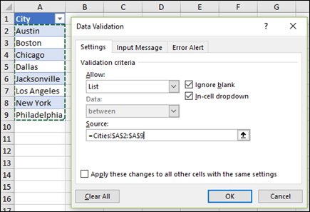
On the Settings tab, click in the Source box, and then on the worksheet that has the entries for your drop-down list, select all of the cells containing those entries. You’ll see the list range in the Source box change as you select.
-
To update all cells that have the same drop-down list applied, check the Apply these changes to all other cells with the same settings box.
-
On the worksheet where you applied the drop-down list, select a cell that has the drop-down list.
-
Go to Data > Data Validation.
-
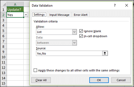
On the Settings tab, click in the Source box, and then change your list items as needed. Each item should be separated by a comma, with no spaces in between like this: Yes,No,Maybe.
-
To update all cells that have the same drop-down list applied, check the Apply these changes to all other cells with the same settings box.
After you update a drop-down list, make sure it works the way you want. For example, check to see if the cell is wide enough to show your updated entries.
If the list of entries for your drop-down list is on another worksheet and you want to prevent users from seeing it or making changes, consider hiding and protecting that worksheet. For more information about how to protect a worksheet, see Lock cells to protect them.
If you want to delete your drop-down list, see Remove a drop-down list.
To see a video about how to work with drop-down lists, see Create and manage drop-down lists.
Edit a drop-down list that’s based on an Excel Table
If you set up your list source as an Excel table, then all you need to do is add or remove items from the list, and Excel will automatically update any associated drop-downs for you.
-
To add an item, go to the end of the list and type the new item.
-
To remove an item, press Delete.
Tip: If the item you want to delete is somewhere in the middle of your list, right-click its cell, click Delete, and then click OK to shift the cells up.
-
Select the worksheet that has the named range for your drop-down list.
-
Do any of the following:
-
To add an item, go to the end of the list and type the new item.
-
To remove an item, press Delete.
Tip: If the item you want to delete is somewhere in the middle of your list, right-click its cell, click Delete, and then click OK to shift the cells up.
-
-
Go to Formulas > Name Manager.
-
In the Name Manager box, click the named range you want to update.
-
Click in the Refers to box, and then on your worksheet select all of the cells that contain the entries for your drop-down list.
-
Click Close, and then click Yes to save your changes.
Tip: If you don’t know what a named range is named, you can select the range and look for its name in the Name Box. To locate a named range, see Find named ranges.
-
Select the worksheet that has the data for your drop-down list.
-
Do any of the following:
-
To add an item, go to the end of the list and type the new item.
-
To remove an item, click Delete.
Tip: If the item you want to delete is somewhere in the middle of your list, right-click its cell, click Delete, and then click OK to shift the cells up.
-
-
On the worksheet where you applied the drop-down list, select a cell that has the drop-down list.
-
Go to Data > Data Validation.
-
On the Settings tab, click in the Source box, and then on the worksheet that has the entries for your drop-down list, Select cell contents in Excel containing those entries. You’ll see the list range in the Source box change as you select.
-
To update all cells that have the same drop-down list applied, check the Apply these changes to all other cells with the same settings box.
-
On the worksheet where you applied the drop-down list, select a cell that has the drop-down list.
-
Go to Data > Data Validation.
-
On the Settings tab, click in the Source box, and then change your list items as needed. Each item should be separated by a comma, with no spaces in between like this: Yes,No,Maybe.
-
To update all cells that have the same drop-down list applied, check the Apply these changes to all other cells with the same settings box.
After you update a drop-down list, make sure it works the way you want. For example, check to see how to Change the column width and row height to show your updated entries.
If the list of entries for your drop-down list is on another worksheet and you want to prevent users from seeing it or making changes, consider hiding and protecting that worksheet. For more information about how to protect a worksheet, see Lock cells to protect them.
If you want to delete your drop-down list, see Remove a drop-down list.
To see a video about how to work with drop-down lists, see Create and manage drop-down lists.
In Excel for the web, you can only edit a drop-down list where the source data has been entered manually.
-
Select the cells that have the drop-down list.
-
Go to Data > Data Validation.
-
On the Settings tab, click in the Source box. Then do one of the following:
-
If the Source box contains drop-down entries separated by commas, then type new entries or remove ones you don’t need. When you’re done, each entry should be separated by a comma, with no spaces. For example: Fruits,Vegetables,Meat,Deli.
-
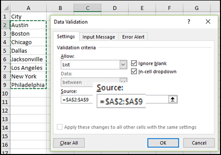
If the Source box contains a reference to a range of cells (for example, =$A$2:$A$5), click Cancel, and then add or remove entries from those cells. In this example, you’d add or remove entries in cells A2 through A5. If the list of entries ends up being longer or shorter than the original range, go back to the Settings tab and delete what’s in the Source box. Then click and drag to select the new range containing the entries.
-
If the Source box contains a named range, like Departments, then you need to change the range itself using a desktop version of Excel.
-
After you update a drop-down list, make sure it works the way you want. For example, check to see if the cell is wide enough to show your updated entries. If you want to delete your drop-down list, see Remove a drop-down list.
Need more help?
You can always ask an expert in the Excel Tech Community or get support in the Answers community.
See Also
Create a drop-down list
Apply Data Validation to cells
Video: Create and manage drop-down lists
Need more help?
Want more options?
Explore subscription benefits, browse training courses, learn how to secure your device, and more.
Communities help you ask and answer questions, give feedback, and hear from experts with rich knowledge.
Author: Oscar Cronquist Article last updated on December 08, 2018
Overview
Updating a list using copy/paste is a boring task. This blog article describes how to update values in a price list with new values.
Sheet 1 is the old price list. It contains 5000 products and amounts.

Sheet2 is the new price list. It contains 2000 random products from the old price list with new prices. (There are no new products)

How to create a new list with the latest prices.
Copy all products from sheet1 into sheet 3

Now let us find out if a new price exists.
Sheet3, formula in B2:
=INDEX(Sheet2!$B$2:$B$2001, MATCH(A2, Sheet2!$A$2:$A$2001, 0)) + ENTER.

Double press with left mouse button on lower right corner of cell B2.

The formula is copied down to last adjacent product.
Sheet3, formula in C2:
=IF(ISERROR(MATCH(A2, Sheet2!$A$2:$A$2001, 0)), INDEX(Sheet1!$B$2:$B$5000, MATCH(A2, Sheet1!$A$2:$A$5000, 0)), INDEX(Sheet2!$B$2:$B$2001, MATCH(A2, Sheet2!$A$2:$A$2001, 0))) + ENTER.
Double press with left mouse button on lower right corner of cell C2 to copy the formula as far down as needed.

I created column B to make sure the values are the same as in sheet2 and to make it easier to understand the formula in cell C2.
Explaining the formula in cell C2
Step 1 — Find out if a new price exists
=IF(ISERROR(MATCH(A2, Sheet2!$A$2:$A$2001, 0)), INDEX(Sheet1!$B$2:$B$5000, MATCH(A2, Sheet1!$A$2:$A$5000, 0)), INDEX(Sheet2!$B$2:$B$2001, MATCH(A2, Sheet2!$A$2:$A$2001, 0)))
Match returns the relative position of an item in (Sheet2!$A$2:$A$2001) that matches a specified value (A2).
MATCH(A2, Sheet2!$A$2:$A$2001, 0) returns #N/A. This means «Product AT» can´t be found in sheet2.
ISERROR(MATCH(A2, Sheet2!$A$2:$A$2001, 0)) returns TRUE.
Step 2 — Identify sheet and price
The formula returned TRUE in cell C2. This means there is no new price. Let´s find the old price in sheet1 instead.
=IF(ISERROR(MATCH(A2, Sheet2!$A$2:$A$2001, 0)), Formula if TRUE, Formula if FALSE)
=IF(ISERROR(MATCH(A2, Sheet2!$A$2:$A$2001, 0)), INDEX(Sheet1!$B$2:$B$5000, MATCH(A2, Sheet1!$A$2:$A$5000, 0)), INDEX(Sheet2!$B$2:$B$2001, MATCH(A2, Sheet2!$A$2:$A$2001, 0)))
INDEX(Sheet1!$B$2:$B$5000, MATCH(A2, Sheet1!$A$2:$A$5000, 0))
MATCH(A2, Sheet1!$A$2:$A$5000, 0) returns 1. «Product AT» is found on the first row on sheet1.
INDEX(Sheet1!$B$2:$B$5000, 1) returns $43,90.
If formula in step 1 had returned False
If the formula had returned False in cell C2, we would need to look for the new price in sheet2.
=IF(ISERROR(MATCH(A2, Sheet2!$A$2:$A$2001, 0)), Formula if TRUE, Formula if FALSE)
=IF(ISERROR(MATCH(A2, Sheet2!$A$2:$A$2001, 0)), INDEX(Sheet1!$B$2:$B$5000, MATCH(A2, Sheet1!$A$2:$A$5000, 0)), INDEX(Sheet2!$B$2:$B$2001, MATCH(A2, Sheet2!$A$2:$A$2001, 0)))
INDEX(Sheet2!$B$2:$B$2001, MATCH(A2, Sheet2!$A$2:$A$2001, 0))
Get excel example file
automate_excel_pricelist.zip (300 KB)
See all How-To Articles
This tutorial demonstrates how to update a drop-down list in Excel and Google Sheets.
Update Drop Down List
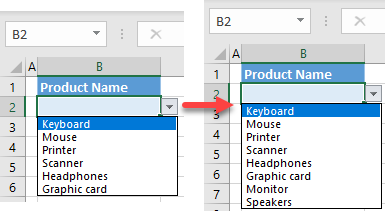
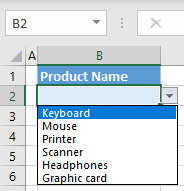
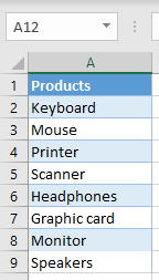
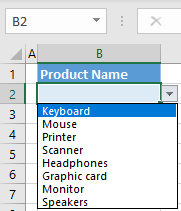
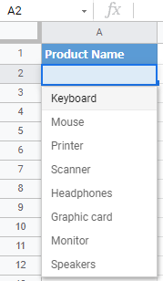
If you have a drop-down list in Excel, you can update the list of items easily. Say you have the following drop-down list in cell B2, containing product names.
This drop down is populated from the range A2:A7 in Sheet2.
To add two new items to the drop-down list (Monitor and Speakers), follow these steps:
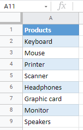
- First, add the new items to the source range in Sheet2 (cells A8 and A9).
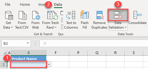
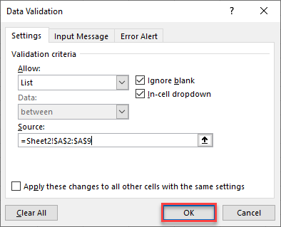
- Now, select a cell with the drop-down data validation rule (cell B2) and in the Ribbon, go to Data > Data Validation.
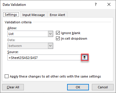
- In the Data Validation window, you can see that the source of the drop-down list is range A2:A7 from Sheet2. To expand this source, click on the arrow next to the range.
- Select the expanded range (A2:A9), and press Enter on the keyboard.
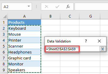
- Now you’re back to the Data Validation window. Click OK to finish.
Now, when you click on the drop down in cell B2, the list includes the newly-added Product items.
Update Drop Down List in Google Sheets
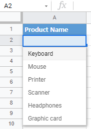
Say you have the same drop-down list with products in Google Sheets.
To update the drop-down list in Google Sheets, follow these steps.
- First, add new items to the range in Sheet2 (here, cells A8 and A9).
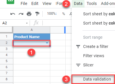
- Select a cell with the drop-down list (A2), and in the Menu, go to Data > Data validation.
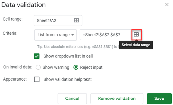
- In the Data validation window, to the right of Criteria, click on the Select data range icon.
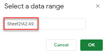
- Select the range with new items (A2:A9, in Sheet2), and click OK.
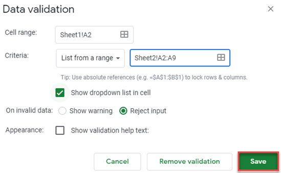
- This takes you back to the Data validation window. Click Save to confirm changes.
The result is the same as in Excel: The drop-down list is updated with new items.
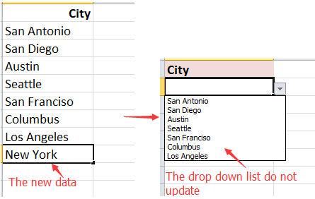
We often create a dropdown list based on certain range in excel to filter value recorded in this data range. Usually the original data range is not fixed, we can add more values in the following cells which are not included in the original data range per our demands, and in this case the dropdown list cannot be updated accordingly due to the range defined during creating dropdown list doesn’t cover the new data. This article will help you to solve this problem by two methods, use OFFSET function in data validation, or create a table and define the table name in advance before create dropdown list.
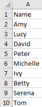
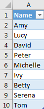
Create a table. It can be seen as the original data.
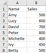
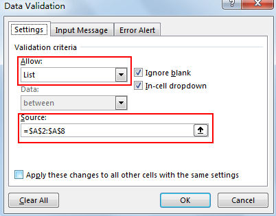
Create a dropdown list based on this range.
Add a new name Serena into A9, and let’s see if the dropdown list is auto updated.
Obviously, the dropdown list is not auto updated per our expect. Now let’s follow below steps to implement this feature.
Table of Contents
- Method 1: Auto Update Dropdown List by OFFSET Function in Excel
- Method 2: Auto Update Dropdown List by Define Table Name in Excel
Method 1: Auto Update Dropdown List by OFFSET Function in Excel
Step 1: Click Data->Data Validation to load Data Validation window. Verify that previous settings are loaded automatically.
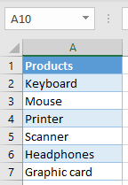
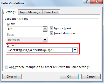
Step 2: In Source textbox, enter =OFFSET($A$2,0,0,COUNTA(A:A)-1). Then click OK to save the update. In this case, $A$2 is the first cell in original data range and it is also the first cell in dropdown list. After entering the formula, we can ignore that row/column range in dropdown list source range.
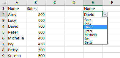
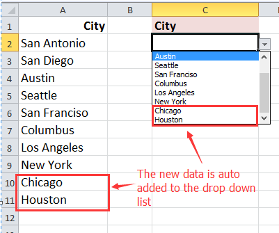
Step 3: Add a new name Tom in A10 to test if above method works.
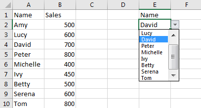
Verify that Tom is auto added in the dropdown list.
Method 2: Auto Update Dropdown List by Define Table Name in Excel
Step 1: Select the range A2:A10 from original data range, see below screenshot.
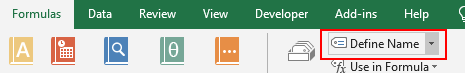
Step 2: Click Formulas->Define Name.
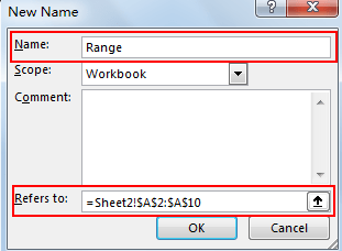
Step 3: In New Name window, enter ‘Range’ in ‘Name’ textbox, keep ‘Refers to’ textbox value (or you can select the range you want to display in dropdown list here), then click OK.
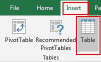
Step 4: Select a cell included in the source data, for example we select David. Then click Insert->Table.
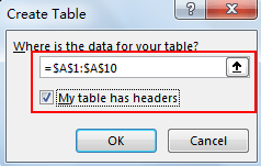
Step 5: In Create Table window, check on the option ‘My table has headers’. Select =$A$1:$A$10 as the table data. Then click OK.
Verify that table is created properly. Name is the header.
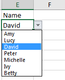
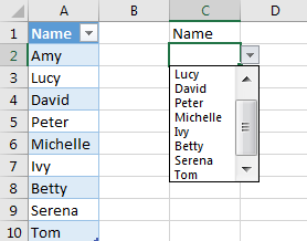
Step 6: Create dropdown list in C2. Click Data->Data Validation. In Data Validation window, in Allow dropdown list select List, in Source textbox, enter =Range. Then click OK. In this case, Range is the defined name in step 3.

Verify that dropdown list is created properly.
Step 7: Input new names Henry and Bobbi into table.
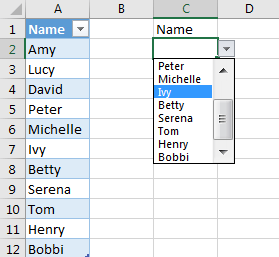
Verify that dropdown list is auto updated accordingly.
В Excel мы обычно создаем выпадающий список для повседневной работы. По умолчанию вы можете добавить новые данные в ячейку из диапазона исходных данных, тогда соответствующий раскрывающийся список будет обновлен автоматически. Но если вы добавляете новые данные в ячейку ниже исходного диапазона данных, относительный раскрывающийся список не может быть обновлен. Здесь я расскажу вам хороший способ автоматического обновления раскрывающегося списка при добавлении новых данных к исходным данным.
Раскрывающийся список автообновлений
 Раскрывающийся список автообновлений
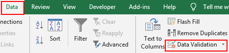
1. Выберите ячейку, в которую хотите поместить раскрывающийся список, и нажмите Данные > проверка достоверности данных > проверка достоверности данных. Смотрите скриншот:

2. в проверка достоверности данных диалоговом окне, щелкните вкладку Настройка и выберите Список от Разрешить список, затем введите = СМЕЩЕНИЕ (2,0,0 $ A $; COUNTA (A: A) -1) в текстовое поле Источник. Смотрите скриншот:
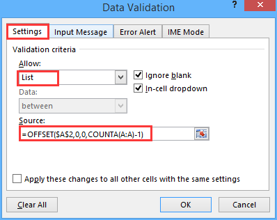
Функции: В приведенной выше формуле A2 — это первая ячейка диапазона данных, с которым вы хотите создать раскрывающийся список, а A: A — местоположение исходных данных столбца.
3. Нажмите OK. Теперь создается автоматически обновляемый раскрывающийся список. А когда вы добавляете новые данные в исходный диапазон данных, раскрывающийся список тем временем обновляется.
Относительные статьи:
- Создать динамический раскрывающийся список
Лучшие инструменты для работы в офисе
Kutools for Excel Решит большинство ваших проблем и повысит вашу производительность на 80%
- Снова использовать: Быстро вставить сложные формулы, диаграммы и все, что вы использовали раньше; Зашифровать ячейки с паролем; Создать список рассылки и отправлять электронные письма …
- Бар Супер Формулы (легко редактировать несколько строк текста и формул); Макет для чтения (легко читать и редактировать большое количество ячеек); Вставить в отфильтрованный диапазон…
- Объединить ячейки / строки / столбцы без потери данных; Разделить содержимое ячеек; Объединить повторяющиеся строки / столбцы… Предотвращение дублирования ячеек; Сравнить диапазоны…
- Выберите Дубликат или Уникальный Ряды; Выбрать пустые строки (все ячейки пустые); Супер находка и нечеткая находка во многих рабочих тетрадях; Случайный выбор …
- Точная копия Несколько ячеек без изменения ссылки на формулу; Автоматическое создание ссылок на несколько листов; Вставить пули, Флажки и многое другое …
- Извлечь текст, Добавить текст, Удалить по позиции, Удалить пробел; Создание и печать промежуточных итогов по страницам; Преобразование содержимого ячеек в комментарии…
- Суперфильтр (сохранять и применять схемы фильтров к другим листам); Расширенная сортировка по месяцам / неделям / дням, периодичности и др .; Специальный фильтр жирным, курсивом …
- Комбинируйте книги и рабочие листы; Объединить таблицы на основе ключевых столбцов; Разделить данные на несколько листов; Пакетное преобразование xls, xlsx и PDF…
- Более 300 мощных функций. Поддерживает Office/Excel 2007-2021 и 365. Поддерживает все языки. Простое развертывание на вашем предприятии или в организации. Полнофункциональная 30-дневная бесплатная пробная версия. 60-дневная гарантия возврата денег.
")
Вкладка Office: интерфейс с вкладками в Office и упрощение работы
- Включение редактирования и чтения с вкладками в Word, Excel, PowerPoint, Издатель, доступ, Visio и проект.
- Открывайте и создавайте несколько документов на новых вкладках одного окна, а не в новых окнах.
- Повышает вашу продуктивность на 50% и сокращает количество щелчков мышью на сотни каждый день!
")
Комментарии (1)
Оценок пока нет. Оцените первым!