
How to recalculate and refresh formulas
- F2 – select any cell then press F2 key and hit enter to refresh formulas.
- F9 – recalculates all sheets in workbooks.
- SHIFT+F9 – recalculates all formulas in the active sheet.
Contents
- 1 How do you get Excel to automatically update formulas?
- 2 How do you manually update formulas in Excel?
- 3 Why is Excel not updating formulas?
- 4 How do I update multiple formulas in Excel?
- 5 How do I permanently enable iterative in Excel?
- 6 What does F9 do in Excel?
- 7 How do you refresh formulas in Excel Mac?
- 8 Why formula is not working in Excel?
- 9 What is enable iterative calculation in Excel?
- 10 How do you update formulas?
- 11 What is the fastest way to change the formula in Excel?
- 12 How do you copy formulas in Excel without changing references?
- 13 How do I update multiple cells at once?
- 14 How do you keep iterative calculations?
- 15 How does a Vlookup work?
- 16 What is the mixed reference?
- 17 What does Alt F11 do in Excel?
- 18 What does Alt F5 do in Excel?
- 19 What does Alt R do?
- 20 How do you refresh a data table in Excel?
How do you get Excel to automatically update formulas?
In the Excel for the web spreadsheet, click the Formulas tab. Next to Calculation Options, select one of the following options in the dropdown: To recalculate all dependent formulas every time you make a change to a value, formula, or name, click Automatic. This is the default setting.
How do you manually update formulas in Excel?
To refresh or recalculate in Excel (when using the F9 for The Financial Edge), use the following keys:
- To refresh the current cell – press F2 + Enter.
- To refresh the current tab – press Shift + F9.
- To refresh the entire workbook – press F9.
Why is Excel not updating formulas?
Excel formulas not updating
When Excel formulas are not updating automatically, most likely it’s because the Calculation setting has been changed to Manual instead of Automatic. To fix this, just set the Calculation option to Automatic again.
How do I update multiple formulas in Excel?
Just select all the cells at the same time, then enter the formula normally as you would for the first cell. Then, when you’re done, instead of pressing Enter, press Control + Enter. Excel will add the same formula to all cells in the selection, adjusting references as needed.
How do I permanently enable iterative in Excel?
Learn about iterative calculation
- If you’re using Excel 2010 or later, click File > Options > Formulas.
- In the Calculation options section, select the Enable iterative calculation check box.
- To set the maximum number of times that Excel will recalculate, type the number of iterations in the Maximum Iterations box.
What does F9 do in Excel?
F9. Calculates the workbook. By default, any time you change a value, Excel automatically calculates the workbook. Turn on Manual calculation (on the Formulas tab, in the Calculation group, click Calculations Options, Manual) and change the value in cell A1 from 5 to 6.
How do you refresh formulas in Excel Mac?
How to Refresh Reports in MS Excel for Mac
- To Refresh the data in the report, click on the Data ribbon button, then click on the Refresh button.
- If the values show as zeros in the pivot tables after refreshing, please check your MacOS language and text settings.
- Related articles.
Why formula is not working in Excel?
Possible cause 1: Cells are formatted as text
Cause: The cell is formatted as Text, which causes Excel to ignore any formulas. This could be directly due to the Text format, or is particularly common when importing data from a CSV or Notepad file. Fix: Change the format of the cell(s) to General or some other format.
What is enable iterative calculation in Excel?
Enabling iterative calculations will bring up two additional inputs in the same menu:
- Maximum Iterations determines how many times Excel is to recalculate the workbook,
- Maximum Change determines the maximum difference between values of iterative formulas.
How to recalculate and refresh formulas
- F2 – select any cell then press F2 key and hit enter to refresh formulas.
- F9 – recalculates all sheets in workbooks.
- SHIFT+F9 – recalculates all formulas in the active sheet.
What is the fastest way to change the formula in Excel?
You can press F2 again to toggle back to Edit mode, to move the text cursor. This toggle allows you to modify formulas by just using the keyboard. The use of F2 will depend on the scenario. Sometimes it’s faster to use the mouse.
How do you copy formulas in Excel without changing references?
Press F2 (or double-click the cell) to enter the editing mode. Select the formula in the cell using the mouse, and press Ctrl + C to copy it. Select the destination cell, and press Ctl+V. This will paste the formula exactly, without changing the cell references, because the formula was copied as text.
How do I update multiple cells at once?
You can drag an area with your mouse, hold down SHIFT and click in two cells to select all the ones between them, or hold down CTRL and click to add individual cells. Then type in your selected text. Finally, hit CTRL+ENTER (instead of enter) and it’ll be entered into all the selected cells. How simple is that?
How do you keep iterative calculations?
In the Excel Options dialog box, click Formulas. In the Calculation options section, select or clear the Enable iterative calculation check box.
How does a Vlookup work?
The VLOOKUP function performs a vertical lookup by searching for a value in the first column of a table and returning the value in the same row in the index_number position.As a worksheet function, the VLOOKUP function can be entered as part of a formula in a cell of a worksheet.
What is the mixed reference?
Mixed reference Excel definition: A mixed reference is made up of both an absolute reference and relative reference. This means that part of the reference is fixed, either the row or the column, and the other part is relative.
What does Alt F11 do in Excel?
F11 Creates a chart of the data in the current range in a separate Chart sheet. Shift+F11 inserts a new worksheet. Alt+F11 opens the Microsoft Visual Basic For Applications Editor, in which you can create a macro by using Visual Basic for Applications (VBA).
What does Alt F5 do in Excel?
h) Alt + Ctrl + Shift + F4: “Alt + Ctrl + Shift + F4” keys closes all open Excel file i.e. these work similar to “Alt + F4” keys. “F5” key is used to display “Go To” dialog box; it will help you in viewing named range. This will restore windows size of the current excel workbook.
What does Alt R do?
Alt+R is a keyboard shortcut most often used to open the Review tab in the Office programs Ribbon.
How do you refresh a data table in Excel?
Manually refresh
To update the information to match the data source, click the Refresh button, or press ALT+F5. You can also right-click the PivotTable, and then click Refresh. To refresh all PivotTables in the workbook, click the Refresh button arrow, and then click Refresh All.
How to fix Excel formulas not calculating (Refresh Formulas)
Formulas are the life and blood of Microsoft Excel.
We use them to add numbers, subtract dates, and even extract texts.
When entering a formula, the result comes almost immediately!
But what happens when it doesn’t?

Obviously, 2+2 = 4! Not 5!
Could we actually be better at basic math than Excel? Probably not 🤣
So, how do you fix a formula that won’t calculate automatically?
In this tutorial, you learn about why your formulas are not updating and how to fix them!
If you want to tag along, download the sample Excel file here.
Let’s dive right into the most common cause of formulas not updating:
Calculation options set to ‘Manual calculation’ mode
What? 😲
Could it really be that simple?
In Excel, it is actually possible to change the calculation setting.
You can check and set the current calculation mode like this:
1. Click the Formulas tab.

2. Click on Calculation Options.

3. Verify that the calculation setting is Automatic.

4. Formulas will not recalculate automatically if Excel is set to Manual calculation mode.
In the practice Excel workbook, the formula in cell C2 is a simple addition formula:
=A2 + B2
You can change the values of A2 & B2 as you wish…

…but the formula result will not change while the setting is still in Manual calc mode.
5. To get the correct result, set the Calculation Options to Automatic calculation mode.

Voila!
Now you can go back to working with Excel as usual!
Alternatively…
You can also change the calculation mode by going into File > More… > Options > Formulas tab.

There are four calculation modes to choose from:
- Automatic – All dependent formulas in the entire workbook are recalculated as cell values change.
- Automatic Except for Data Tables – Same as Automatic. But Data Tables are only recalculated if a cell inside the table has changed
- Manual – The entire workbook is only recalculated if you press F9. Or if you click Calculate Now or Calculate Sheet in the Formulas ribbon
- Manual / Recalculate before saving – Same as Manual calc mode. But formulas are also recalculated every time you save the file.
But why did my Calculation Mode change? 🤔
Bear in mind that the calculation setting is an application-level setting.
If you change the Calculation Mode, this applies to the entire workbook and all other open workbooks.
Also, Excel uses the last saved calculation mode of the first workbook opened. All workbooks opened in the same session will use the same mode.
Try to open the practice Excel file without any other open workbooks.
You will notice that it opens in Manual calculation mode. This was the setting it was last saved with.You can learn more about Calculation Mode behavior from the official Microsoft website.
Running a macro can also change the calculation mode
This is especially true if the macro or VBA developer used any of the lines below:
- Application.Calculation = xlCalculationAutomatic
- Application.Calculation = xlCalculationManual
If you are not working with a macro-enabled workbook, then you can definitely rule this out!
Why use ‘Manual calculation’ mode?
Well, if you are working with a large amount of data, you may notice a slight lag or delay in Excel. 🐌
This is usually caused by Excel automatically recalculating formulas with every change.
This can slow your work down quite a lot.
💡 So, you can change to Manual calculation mode as you enter or change data and switch back to Automatic later on.
Manual calculation shortcuts
In Manual mode, you can refresh formulas by pressing F9.
You can also click the Calculate Now or Calculate Sheet buttons in the Formulas ribbon.

This can help you save time and avoid the stress of waiting for Excel to finish updating formulas!
Cell is formatted as text
Wrong cell format could also prevent the automatic calculation of a formula.
Take a look at the worksheet “Example-Text Format” of the practice Excel file.
The Excel formula in cell C2 is exactly the same as the formula in cell C2 of the worksheet “Example-Calc Mode”.

But in the worksheet “Example-Text Format”, it only shows the formula and not the value.
Even if the Excel workbook is not set to Manual calc mode, the cell value will not update.
To fix this, you can change the cell format:
1. In the Home ribbon, click on the Number Format drop-down.

2. Select your desired number format.
The General and Number formats are usually used for calculations.

3. Double-click on the cell or click the formula bar.
The cell references should are now highlighted as they normally are in an Excel formula.

4. Hit Enter to get the result!

Excel set to show formulas instead of results
Another thing to consider is the Show Formulas feature.
If this is ON, cells will show the formulas instead of the values.
You can toggle it ON and OFF by clicking the Show Formulas button in the Formulas ribbon.

You can also use these shortcuts to toggle display between formulas and values:
- On Windows: Use Ctrl + ‘
- On Mac: Use ^ + `
The Show Formulas feature changes the display between formula and cell value.
This is so you can check for errors and inconsistencies in the entire workbook.
Try it out for yourself!
There’s a circular reference somewhere in your workbook
Are you still having issues even after the above fixes?
If so, you might have a circular reference in your workbook.
This is when a formula refers to its own cell either directly or indirectly.

In the worksheet “Example-Circ Ref 1” of the practice workbook, we have a simple SUM formula at cell B6.
The formula includes itself in the calculation “=SUM(B2:B6)”.
Thus, the formula will not calculate correctly.
You can identify and fix formulas with circular references like this:
1. In the Formulas ribbon, click on Error Checking.

2. This opens a drop-down. Select Circular References.
It will then show you a list of cells with circular references that need fixing.

Alternative method to check for circular references
You can check the bottom left corner of the Excel window.
It will display a message like the one below if there are circular references.

You may also see blue lines that show formulas dependent on one another.
Open the worksheet “Example-Circ Ref 2” for this next example.
Here you have slightly more complex formulas involving a budget spreadsheet.

The example above shows two ways to calculate the Contingency and Total Project Cost.
- In Calculation A: The formula for the Total Project Cost at cell B9 is “=SUM(B4:B8)” while the formula for the 5% Contingency at cell B7 is “=B9*0.05”.
Thus, cells B7 and B9 have formulas dependent on one another. This is a circular reference and the Excel formulas default to zero. - In Calculation B: This circular reference is fixed by having a Sub-total at cell F7.
This way, the Contingency can be computed at cell F8 and the Total Project Cost is now just “=F7+F8”.
There are no circular references here so the values are computed correctly!
You can learn more about this and other examples in our tutorial about circular references here.
That’s it – Now what?
You are now familiar with the four most common reasons why your Excel formulas won’t automatically calculate.
Reason number 1, the Calculation Mode setting, is almost always the culprit ⚙️
This is especially true when you open workbooks downloaded from the Internet. Or if you open workbooks from a different computer.
You will encounter wrong cell Text formatting, Show Formulas toggle, and Circular References less often.
But all this doesn’t matter if you don’t know how to actually build formulas and functions that make your work easier.
Functions like IF, SUMIF, and VLOOKUP.
You learn all these (and more!) in my free 30-minute training. Click here to enroll.
Other relevant resources
You just read what to do when the formulas don’t update. But what if you get different error messages like #VALUE, #REF, and #NAME?
That’s an entirely different part of Excel and you can read all about that here.
Or you can read here how to use IFERROR or ISERROR to work with errors and have formulas work all the time!
Kasper Langmann2022-09-26T18:10:39+00:00
Page load link
Содержание
- Change formula recalculation, iteration, or precision in Excel
- Need more help?
- Automatic recalculation of formulas in Excel and manually
- Automatic and manual conversion
- How to display to a formula in the Excel cell
Change formula recalculation, iteration, or precision in Excel
To use formulas efficiently, there are three important considerations that you need to understand:
Calculation is the process of computing formulas and then displaying the results as values in the cells that contain the formulas. To avoid unnecessary calculations that can waste your time and slow down your computer, Microsoft Excel automatically recalculates formulas only when the cells that the formula depends on have changed. This is the default behavior when you first open a workbook and when you are editing a workbook. However, you can control when and how Excel recalculates formulas.
Iteration is the repeated recalculation of a worksheet until a specific numeric condition is met. Excel cannot automatically calculate a formula that refers to the cell — either directly or indirectly — that contains the formula. This is called a circular reference. If a formula refers back to one of its own cells, you must determine how many times the formula should recalculate. Circular references can iterate indefinitely. However, you can control the maximum number of iterations and the amount of acceptable change.
Precision is a measure of the degree of accuracy for a calculation. Excel stores and calculates with 15 significant digits of precision. However, you can change the precision of calculations so that Excel uses the displayed value instead of the stored value when it recalculates formulas.
As calculation proceeds, you can choose commands or perform actions such as entering numbers or formulas. Excel temporarily interrupts calculation to carry out the other commands or actions and then resumes calculation. The calculation process may take more time if the workbook contains a large number of formulas, or if the worksheets contain data tables or functions that automatically recalculate every time the workbook is recalculated. Also, the calculation process may take more time if the worksheets contain links to other worksheets or workbooks. You can control when calculation occurs by changing the calculation process to manual calculation.
Important: Changing any of the options affects all open workbooks.
Click the File tab, click Options, and then click the Formulas category.
In Excel 2007, click the Microsoft Office Button, click Excel Options, and then click the Formulas category.
Do one of the following:
To recalculate all dependent formulas every time you make a change to a value, formula, or name, in the Calculation options section, under Workbook Calculation, click Automatic. This is the default calculation setting.
To recalculate all dependent formulas — except data tables — every time you make a change to a value, formula, or name, in the Calculation options section, under Workbook Calculation, click Automatic except for data tables.
To turn off automatic recalculation and recalculate open workbooks only when you explicitly do so (by pressing F9), in the Calculation options section, under Workbook Calculation, click Manual.
Note: When you click Manual, Excel automatically selects the Recalculate workbook before saving check box. If saving a workbook takes a long time, clearing the Recalculate workbook before saving check box may improve the save time.
To manually recalculate all open worksheets, including data tables, and update all open chart sheets, on the Formulas tab, in the Calculation group, click the Calculate Now button.

To manually recalculate the active worksheet and any charts and chart sheets linked to this worksheet, on the Formulas tab, in the Calculation group, click the Calculate Sheet button.
Tip: Alternatively, you can change many of these options outside of the Excel Options dialog box. On the Formulas tab, in the Calculation group, click Calculation Options, and then click Automatic.
Note: If a worksheet contains a formula that is linked to a worksheet that has not been recalculated and you update that link, Excel displays a message stating that the source worksheet is not completely recalculated. To update the link with the current value stored on the source worksheet, even though the value might not be correct, click OK. To cancel updating the link and use the previous value obtained from the source worksheet, click Cancel.
Recalculate formulas that have changed since the last calculation, and formulas dependent on them, in all open workbooks. If a workbook is set for automatic recalculation, you do not need to press F9 for recalculation.
Recalculate formulas that have changed since the last calculation, and formulas dependent on them, in the active worksheet.
Recalculate all formulas in all open workbooks, regardless of whether they have changed since the last recalculation.
Check dependent formulas, and then recalculate all formulas in all open workbooks, regardless of whether they have changed since the last recalculation.
Click the File tab, click Options, and then click the Formulas category.
In Excel 2007, click the Microsoft Office Button, click Excel Options, and then click the Formulas category.
In the Calculation options section, select the Enable iterative calculation check box.
To set the maximum number of times Excel will recalculate, type the number of iterations in the Maximum Iterations box. The higher the number of iterations, the more time Excel will need to recalculate a worksheet.
To set the maximum amount of change you will accept between recalculation results, type the amount in the Maximum Change box. The smaller the number, the more accurate the result and the more time Excel needs to recalculate a worksheet.
Note: Solver and Goal Seek are part of a suite of commands sometimes called what-if analysis tools. Both commands use iteration in a controlled way to obtain desired results. You can use Solver when you need to find the optimum value for a particular cell by adjusting the values of several cells or when you want to apply specific limitations to one or more of the values in the calculation. You can use Goal Seek when you know the desired result of a single formula but not the input value the formula needs to determine the result.
Before you change the precision of calculations, keep in mind the following important points:
By default, Excel calculates stored, not displayed, values
The displayed and printed value depends on how you choose to format and display the stored value. For example, a cell that displays a date as «6/22/2008» also contains a serial number that is the stored value for the date in the cell. You can change the display of the date to another format (for example, to «22-Jun-2008»), but changing the display of a value on a worksheet does not change the stored value.
Use caution when changing the precision of calculations
When a formula performs calculations, Excel usually uses the values stored in cells referenced by the formula. For example, if two cells each contain the value 10.005 and the cells are formatted to display values in currency format, the value $10.01 is displayed in each cell. If you add the two cells together, the result is $20.01 because Excel adds the stored values 10.005 and 10.005, not the displayed values.
When you change the precision of the calculations in a workbook by using the displayed (formatted) values, Excel permanently changes stored values in cells from full precision (15 digits) to whatever format, including decimal places, is displayed. If you later choose to calculate with full precision, the original underlying values cannot be restored.
Click the File tab, click Options, and then click the Advanced category.
In Excel 2007, click the Microsoft Office Button, click Excel Options, and then click the Advanced category
In the When calculating this workbook section, select the workbook you want and then select the Set precision as displayed check box.
Although Excel limits precision to 15 digits, that doesn’t mean that 15 digits is the limit of the size of a number you can store in Excel. The limit is 9.99999999999999E+307 for positive numbers, and -9.99999999999999E+307 for negative numbers . This is approximately the same as 1 or -1 followed by 308 zeros.
Precision in Excel means that any number exceeding 15 digits is stored and shown with only 15 digits of precision. Those digits can be in any combination before or after the decimal point. Any digits to the right of the 15th digit will be zeros. For example, 1234567.890123456 has 16 digits (7 digits before and 9 digits after the decimal point). In Excel, it’s stored and shown as 1234567.89012345 (this is shown in the formula bar and in the cell). If you set the cell to a number format so that all digits are shown (instead of a scientific format, such as 1.23457E+06), you’ll see that the number is displayed as 1234567.890123450. The 6 at the end (the 16th digit) is dropped and replaced by a 0. The precision stops at the 15th digit, so any following digits are zeros.
A computer can have more than one processor (it contains multiple physical processors) or can be hyperthreaded (it contains multiple logical processors). On these computers, you can improve or control the time it takes to recalculate workbooks that contain many formulas by setting the number of processors to use for recalculation. In many cases, portions of a recalculation workload can be performed simultaneously. Splitting this workload across multiple processors can reduce the overall time it takes complete the recalculation.
Click the File tab, click Options, and then click the Advanced category.
In Excel 2007, click the Microsoft Office Button, click Excel Options, and then click the Advanced category.
To enable or disable the use of multiple processors during calculation, in the Formulas section, select or clear the Enable multi-threaded calculation check box.
Note This check box is enabled by default, and all processors are used during calculation. The number of processors on your computer is automatically detected and displayed next to the Use all processors on this computer option.
Optionally, if you select Enable multi-threaded calculation, you can control the number of processors to use on your computer. For example, you might want to limit the number of processors used during recalculation if you have other programs running on your computer that require dedicated processing time.
To control the number of processors, under Number of calculation threads, click Manual. Enter the number of processors to use (the maximum number is 1024).
To ensure that older workbooks are calculated correctly, Excel behaves differently when you first open a workbook saved in an earlier version of Excel than when you open a workbook created in the current version.
When you open a workbook created in the current version, Excel recalculates only the formulas that depend on cells that have changed.
When you use open a workbook that was created in an earlier version of Excel, all the formulas in the workbook — those that depend on cells that have changed and those that do not — are recalculated. This ensures that the workbook is fully optimized for the current Excel version. The exception is when the workbook is in a different calculation mode, such as Manual.
Because complete recalculation can take longer than partial recalculation, opening a workbook that was not previously saved in the current Excel version can take longer than usual. After you save the workbook in the current version of Excel, it will open faster.
In Excel for the web, a formula result is automatically recalculated when you change data in cells that are used in that formula. You can turn this automatic recalculation off and calculate formula results manually. Here’s how to do it:
Note: Changing the calculation option in a workbook will affect the current workbook only, and not any other open workbooks in the browser.
In the Excel for the web spreadsheet, click the Formulas tab.
Next to Calculation Options, select one of the following options in the dropdown:
To recalculate all dependent formulas every time you make a change to a value, formula, or name, click Automatic. This is the default setting.
To recalculate all dependent formulas — except data tables — every time you make a change to a value, formula, or name, click Automatic Except for Data Tables.
To turn off automatic recalculation and recalculate open workbooks only when you explicitly do so, click Manual.
To manually recalculate the workbook (including data tables), click Calculate Workbook.
Note: In Excel for the web, you can’t change the number of times a formula is recalculated until a specific numeric condition is met, nor can you change the precision of calculations by using the displayed value instead of the stored value when formulas are recalculated. You can do that in the Excel desktop application though. Use the Open in Excel button to open your workbook to specify calculation options and change formula recalculation, iteration, or precision.
Need more help?
You can always ask an expert in the Excel Tech Community or get support in the Answers community.
Источник
Automatic recalculation of formulas in Excel and manually
Excel by default recalculates all formulas in all sheets of all open books after each introduction of data. The most swell possibility of Excel – is the automatic recounting by formulas. If the sheet contains hundreds or thousands of formulas, the automatic recalculation starts to noticeably slow down the process of working with the program. This ability of spreadsheets increased people’s productivity in dozens of times.
After all, with manual calculation we need to enter each time not only numbers but mathematical operations, do not get confused, constantly placing intermediate results in memory and so on. In our case, we create formulas and then simply change the numbers — everything will automatically be counted again. Well, if the changes are small, it is even better — even to introduce less of data.
Let`s contemplate, how you can customize Excel to improve its performance and unhindered working.
Automatic and manual conversion
For a book that contains hundreds of compound formulas, you can turn against to the recalculation on requirement of a user. For this:
- You need to enter the formula on a blank sheet (so that you can check how this example works).
- You need to select the tool: «Formulas» – «Calculation Options» – «Manual».
- Make sure that now after entering the data into the cell (for example, the number 7 instead of 1 in the cell A2 as in the draught), the formula does not automatically recalculate the result – while the user does not press the F9 key (or SFIFT + F9).
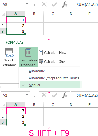
Pay attention! The shortcut F9 performs recalculation in all book formulas on all sheets. There is Combination of hot keys SHIFT + F9 performs recalculation only on the current sheet.
If the sheet does not contain a lot of formulas, that`s why the recalculation can inhibit to Excel. That`s why it makes no sense to use the above described example, but for the future it still worth knowing for you about this possibility: because after all, over time you will have to deal with complex tables with a lot of formulas.
Furthermore, this function can be turned on accidentally and you need to know where to turn it off for the standard operating mode.
How to display to a formula in the Excel cell
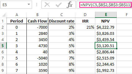
In the Excel cells, we can see the result of the calculations only. The formulas themselves can be seen in the formula line (separately). But sometimes we need to simultaneously view all functions in cells (for example, to compare them, and so forth).
To visually display the example of this lesson, we need this sheet containing the formulas:
We change the Excel settings accordingly so that the cells display the formulas, but not the result of their calculation.
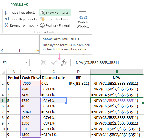
To achieve this result, you need to select the tool: «Formulas» – «Show Formulas»» (in the section «Formulas Auditing»). To exit this display mode, you should to select this implement again.
You can also use the shortcut keys combination CTRL + `(above the Tab key). This combination works in switch mode, that is, you need to press this key repeatedly and returns to the normal display mode of calculation results in cells.
The notation. All the above described actions apply only to the mode of displaying cells of one sheet. That is, on other sheets, if necessary, you need to perform these actions again.
Источник
Hello, time for more #formulafriday fun with Excel Formulas. Do you ever need to update multiple Excel formulas in Excel? If so, you’ll be happy to know that there is an easy way to do this. In this blog post, we will show you how to edit multiple formulas in Excel. Sometimes, you just need a faster way to do stuff in Excel, especially when it comes to creating and updating formulas. So, here is a way to update multiple formulas in Excel really fast using a method you have probably used before, but maybe not for updating formulas.

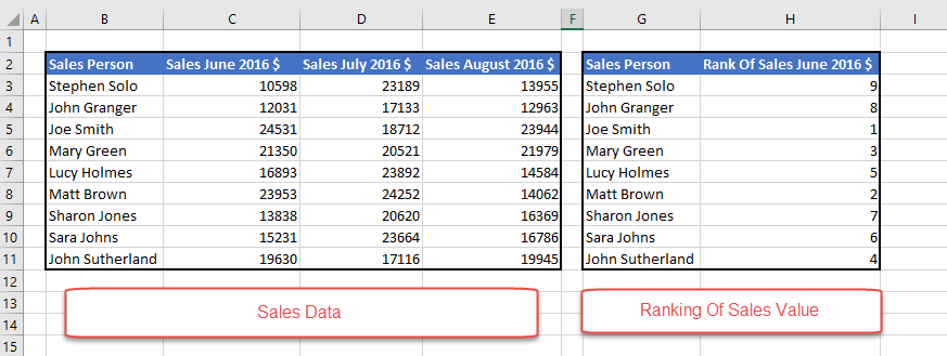
I will share with the process I used on my own Excel workbooks. My Excel workbook calculated the value of sales generated per sales person. These sale are then ranked each month over a period of 3 individual months.
Example Formula.
I have my formula set up to calculate the descending rank (the highest value sales are awarded the highest rank – or lowest value!) for the month of June 2016 as below.
=RANK(C3,$C$3:$C$11)
If I want to now show the ranking of July 2016 I do not need to re write my formulas, I can simply use Find and Replace method. Yes, the simple and often used feature in Excel.
Using Find And Replace To Update The Formulas.
- Select the cells you want to use Find and Replace in – in my example it is Column H
- Hit CTRL+H to bring up the Find & Replace Dialog Box
- On the Find Tab, we can type C
- Hit the Options Tab
- Select Within Sheet – By Columns – Look In – Formulas
- Select the Replace Tab – Type D
- Hit Replace All
Note- Any cells that ou have highighted that contain C will be updated.
- Fially, job done – all of my cells have been updated.
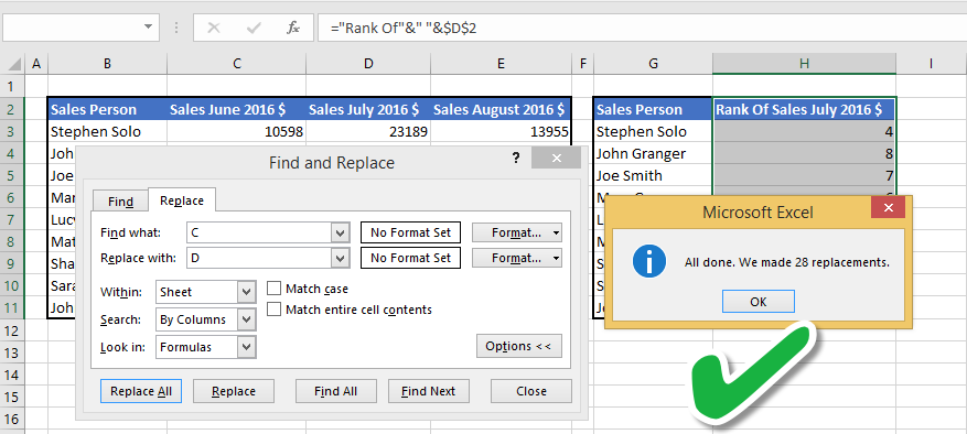
That was easy wasn’t it?. I can then again just update to show August 2016 ranking by using Find & Replace to find D and replace with E.
Have you ever had to edit a lot of Excel formulas at once? Maybe you copied and pasted them from one sheet to another, or maybe you just had a lot of cells that needed the same formatting change. In any case, if you’ve ever done this kind of bulk editing, then you know it can be a pain. Especially if you have to do it over and over again. I hope you found this method quick and easy.
More Excel Formula Tips
Dont forget to sign up to the Excel at Excel Newletter for 3 free Excel tips the first Wednesday of the month. Just click on the Sign Up Form to the right or use the link below.
Why not bookmark my Formula Friday and Macro Monday pages. I update them every week with new Excel tutorials.


This Excel tutorial explains how to write a macro to update all formulas to reference data in a particular column in Excel 2003 and older versions (with screenshots and step-by-step instructions).
Question: In Microsoft Excel 2003/XP/2000/97, I want to create a macro button that when clicked will update all formulas to reference data in a particular column. How can I do this?
Answer: This can be done with a macro.
Let’s look at an example.
Download Excel spreadsheet (as demonstrated below)
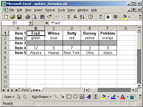
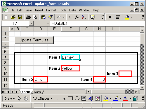
In our spreadsheet, we have two sheets called Form and Data. On the sheet called Data, we’ve placed information in columns B to F. This will be the information referenced by all formulas in the spreadsheet.

The sheet called Form is where the formulas reside. Each cell with a red border contains a formula that references data on the Data sheet.
We’ve placed a button on the Form sheet that when clicked will prompt for the column that all formulas will reference.
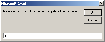
In our example, we’ve chosen to have all formulas reference the data in column E on the Data sheet.
The macro will then replace all formulas on the Form sheet. When it has completed, you will see the following message box appear:
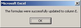
Now when you return to the spreadsheet, you can see that all of the formulas now reference column E on the Data sheet.
To view the macro, press Alt+F11 and double-click on the module called Module1 in the left window.
Macro Code
This macro code looks like this:
Sub UpdateFormulas()

   Dim LColumnLetter As String
   LColumnLetter = InputBox("Please enter the column letter to update the formulas.")

   Sheets("Form").Select

   'All following code will copy a formula into the destination if the source
   'has a value. I f the source does not have a value, it will copy a blank to
   'the destination.

   'Item #1
   Range("F7").Select
   If IsEmpty(Range("Data!" & LColumnLetter & "1").Value) Then
      ActiveCell.Value = ""
   Else
      ActiveCell.Formula = "=Data!" & LColumnLetter & "1"
   End If

   'Item #2
   Range("F9").Select
   If IsEmpty(Range("Data!" & LColumnLetter & "2").Value) Then
      ActiveCell.Value = ""
   Else
      ActiveCell.Formula = "=Data!" & LColumnLetter & "2"
   End If

   'Item #3
   Range("J10").Select
   If IsEmpty(Range("Data!" & LColumnLetter & "3").Value) Then
      ActiveCell.Value = ""
   Else
      ActiveCell.Formula = "=Data!" & LColumnLetter & "3"
   End If

   'Item #4
   Range("H11").Select
   If IsEmpty(Range("Data!" & LColumnLetter & "4").Value) Then
      ActiveCell.Value = ""
   Else
      ActiveCell.Formula = "=Data!" & LColumnLetter & "4"
   End If

   'Item #5
   Range("D11").Select
   If IsEmpty(Range("Data!" & LColumnLetter & "5").Value) Then
      ActiveCell.Value = ""
   Else
      ActiveCell.Formula = "=Data!" & LColumnLetter & "5"
   End If

   'Reposition back on item #1
   Range("F7").Select

   MsgBox ("The formulas were successfully updated to column " & LColumnLetter & ".")

End Sub