Doing some reasoning here so bear with my guess at what precisely you are doing and what you are doing it with.
It SEEMS like you filled column A with whatever, 1-1000, just «dummy», holding pattern values and things went south. That strongly implies you have the formulas in all the other cells to the right of what you filled, hence all the ugly stuff. So my first tack here will be to address that and show you a trick to make it all nice-nice.
When you take an entire formula, simple or complex, that does something you wish but does not handle all the dressing it up to look nice stuff, or some of the «well now and then…» stuff, that’s called «wrapping the formula» with some new function. Simple example: you do something that ends up with a string as a result but there are unfortunate spaces at the beginning or end, or multiple spaces together in the middle. You «wrap» everything so far with the TRIM() function so it strips out those offending spaces.
In this case, you have the formulas in place but don’t want their mess showing unless there’s a real value in column A. So wrap them (Just have to do it on the first row of them, the copy and paste down however far you feel will let you add data without other work for a decent while. Maybe a hundred rows? Maybe the thousand?) with the following IF() function:
=IF(A4="","", (what you had goes here) )
So all the cells in row 4 would look to see if A4 has an entry. If not, they all return «» (nothing, a blank-looking cell). When A4 DOES have something in it, they show the working formula’s result all nice-looking and such.
However, there is something called a «Table» which was invented PRECISELY for the problem you are having. You’d have to highlight and Delete all the formulas in those cells you aren’t using yet (including the dummy stuff in column A), just leaving formulas where real column A data exists. All the rows below cleared out with Delete.
Then select any cell IN the real data that exists, or highlight it all including headers, then go to your Ribbon and click on INSERT. The first section is the Tables section and the rightmost icon there, the third from the left, is «Table» — click it. It will open a small (really small) dialogue box with two things in it. First is Excel’s guess at just what cells make up your table. It’s usually pretty spot on unless you have stuff butted up to those cells which will confuse it. If it looks correct, continue on. If not, use your mouse to highlight everything, including your headers, so Excel can’t get it wrong. Next, if you DO have headers, click to fill the box under that by «My table has headers», then click OK and you’re done.
Now, when you enter something in the column A cell of a row, the rest of the row will fill down automatically with the formulas. That’s why you had to get rid of all the muck you didn’t like the look of anyway. You enter something in the A-cell and all the rest instantly fill. Nice. Some little points… I DO mean the next row. Not 40 empty rows and then you fill in the A-cell of the 41st. That’s a non-starter… Also, if your formula needs to change for any reason, it’s a nightmare. You’ll change a cell’s formula, then see the old formula fill in when you use the next row. It’s complicated how to fix that. One thought for your stated use here would be if you use this over time, tax rates could change. The suggestion would be to make little tax rate lookup tables elsewhere, and in each cell’s formula, use a lookup function, like XLOOKUP() or VLOOKUP() to look them up based upon a date (could need a column for the dates, eh?). That way, you can change or add to those little tables and the formula in your Table would not change.
Third best would be copying a row of formulas down each time you need a new row. Several ways you could do that. Aside from the obvious (highlight, copy, paste, right?) you can fill down each time you need to, just highlight as if about to copy and paste, then use the fill tool. You could even do something esoteric like define a Named Range using relative referencing that is the row you are on, except for the A-cell in that row, and then each time you need a new row, select a cell in a used row, then use the range box above A1, left of the F2-Editing bar to show and select that range by double clicking it from the box that drops down. That’d highlight the current row and you could copy, then go to a blank row and paste. You know, so you could save the awful effort of highlighting the row of formulas ’cause that’d do that for you.
Point is, that ain’t the most fun of options. So use one of the first two, ESPECIALLY converting to a Table. Tables have other advantages too, though none would really look like they’d matter for your use here.
TABLES… I’m not their biggest fan, but that is so incredibly precisely what you need here and so easy to set up. Oh, just accept whatever Styling it wants to do. Change it later if you wish. Walk before running, eh?
I am using all the solutions that appear in:
How to refresh ALL cell through VBA
Getting Excel to refresh data on sheet from within VBA
ActiveSheet.EnableCalculation = False
ActiveSheet.EnableCalculation = True
or
Application.Calculate
or
Application.CalculateFull
None of them works in Excel 2010. When I go to the cell and right click refresh it works. How can I refresh within VBA?
Sheets("Name_of_sheet").Range("D424").Refresh raises an
exception 438
Questions:
- How can I make the script support Excel 2003, 2007, 2010?
- How can I choose the source file to refresh from using VBA?
EDIT:
-
I want to simulate a right mouse click and choose refresh in the menu in
worksheet 3. That is the entire story. -
I work on an Excel file created 10 years ago. When opening in Excel 2010, I can go to a cell and right click on it and choose refresh and then choose the .txt file to refresh from. I am trying to do it automatically within VBA.
asked Nov 22, 2012 at 13:39
6
You could try using Application.Calculation
Application.Calculation = xlCalculationManual
Application.Calculation = xlCalculationAutomatic
answered Nov 22, 2012 at 13:42
4
For an individual cell you can use:
Range("D13").Calculate
OR
Cells(13, "D").Calculate
0x90
38.9k36 gold badges163 silver badges244 bronze badges
answered Nov 22, 2012 at 13:46
InContextInContext
2,46112 silver badges24 bronze badges
1
I finally used mouse events and keystrokes to do it:
Sheets("worksheet34").Select
Range("D15").Select
Application.WindowState = xlMaximized
SetCursorPos 200, 600 'set mouse position at 200, 600
Call mouse_event(MOUSEEVENTF_RIGHTDOWN, 0, 0, 0, 0) 'click left mouse
Application.SendKeys ("R")
answered Nov 29, 2012 at 5:52
0x900x90
38.9k36 gold badges163 silver badges244 bronze badges
2
just a reminder;
be careful when using
Application.Calculation = xlCalculationManual
Application.Calculation = xlCalculationAutomatic
this sets the entire excel application to calculate formula’s either automatically or manually. If you use
Application.Calculation = xlCalculationManual
you’ll notice your automatic formulas no longer work.
cheers
answered Feb 16, 2016 at 17:53
You can force excel to recalculate a cell or range of cells by marking the cell/range as dirty.
Example :
' Recalculate Column D4 to D24
Sheets("Name_of_sheet").Range("D4:D24").Dirty
or
' Recalculate Cell D4<br>
Sheets("Name_of_sheet").Range("D4").Dirty<br>
Ike
7,8904 gold badges11 silver badges29 bronze badges
answered Sep 5, 2021 at 11:16
Application.Calculate didn’t work for my function. Not even when followed by DoEvents.
What I found that works is to re-enter the formula in the cell.
A simple way to get the formula is to start recording a macro, use F2 to edit the cell, then press enter. The macro will make a great copy of the function text with all needed quotes.
Below is an example.
Sheets("Name_of_sheet").Range("D424").FormulaR1C1 = "=now()"
svyat1s
8689 gold badges12 silver badges21 bronze badges
answered Mar 5, 2021 at 19:36
Cells(x, y).Select
ActiveCell.FormulaR1C1 = Selection.Value
works perfectly for me
answered Aug 2, 2022 at 20:21
I have a long «macro» in a workbook > 20 MB, tens of thousands of lines, that calls a dll written in Fortran. None of these methods worked:
Call Application.Calculate
Call Application.CalculateFull
Call Application.CalculateFullRebuild
Re-entering the formula
Range.Dirty

Application.Calculation = xlCalculationManual
Application.Calculation = xlCalculationAutomatic

ThisWorkbook.ActiveSheet.EnableCalculation = False
ThisWorkbook.ActiveSheet.EnableCalculation = True
This worked:
On Error Resume Next
Application.SendKeys "{F2}{Enter}{NumLock}"  'SendKeys turns off NumLock for some reason
On Error GoTo 0
This even worked when a chart was selected.
answered Feb 9 at 14:47
Rocky ScottRocky Scott
4364 silver badges13 bronze badges
There’s a quirk with Microsoft Excel 2010 (and possibly other versions) where custom number formats don’t get applied to existing data. This quick fix can save you from the tedium of re-entering thousands of rows of data.
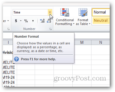
When entering numerical data in Excel, it helps to format it according to the type of data. Formatting a cell according to its data type—e.g., percentage, currency, date, or text—helps drive consistency and accuracy in displaying and working with your data. If you know from the get-go what format your data should be in, it’s relatively simple to choose a number format for the entire column before entering your data. Just select a column and choose a number format from the Number pane in the Home ribbon:
However, things can become troublesome when trying to apply number formatting to an existing range of data. You can update the format of a cell, but sometimes it won’t automatically refresh with the new formatting. This stubbornness usually happens when choosing a custom number format. You can update it by double-clicking the cell, making no changes, and then press Enter, but this can be very tedious. This process is particularly troublesome when importing significant amounts of data.
If you find yourself in this boat, try this trick:
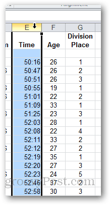
Start with a range of pre-entered data. In this example, we’re using a column that’s entered as text. We want to give it custom formatting so it looks more like a time from a stopwatch. We want to give it the format: [h]:mm:ss
To do this, start by selecting the column.
Then, click the drop-down in the Number pane of the Home ribbon. Choose More number formats. Or, if you want, choose one of the presets.
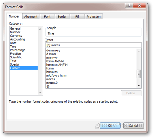
Choose Custom and type in the format you want to use for the numbers. Click OK.
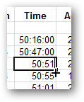
Notice nothing has changed, even though it shows “Custom” in the Number Format drop-down.
If you edit the cell and press enter, the new format takes effect. But with hundreds of rows of data, this will take forever.
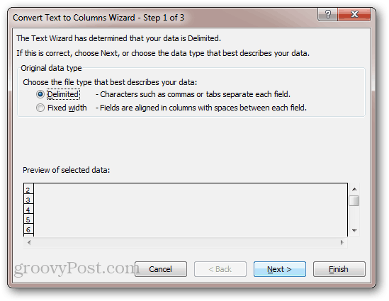
To speed things up, select the column, go to the Data ribbon, and click Text to Columns.
Choose Delimited and click Next.
Uncheck all the delimiters and click Next.
The number formatting of all the cells will update.
This trick is a bit of a hack, but it works. It takes all the values from each row and then re-enters them into the cells automatically. For this reason, this trick will not work for cells that are formulas. If you have formulas, pressing F9 should recalculate the sheet and update the number format. But in my experience, I haven’t had this problem with formulas.
When you try to update cells in Excel using Power Automate you could use the Update a row action.
Update a cell in Excel
In the past I’ve used MS Graph to do things with Excel spreadsheets with Flow.
When you use the update a row action to update cells in Excel, like with all other actions in this connector, you will need a table in your Excel spreadsheet. One additional requirement is needed for the update a row action.
You will need a key column with unique values.
In my example below I created a column key and populate this column with a number.
Now as I run my flow my row with the key equals 1 is updated.
Unique Key column
It is important that you have a Key column that is unique. When I updated the row with Key set to 1 while I had multiple rows having a key of 1 only the first row was updated.
Therefore make sure that you key column is unique and then this update a row action can be very useful.

Posted on Thursday, September 29th, 2011 at 7:01 am by .
I will start with a citation: “I am reading a sheet from an Excel File… I am pooling (with a While loop) the entire worksheet to process each cell … The problem is that it is VERY SLOW because the file is huge… Is there a faster way to read the information?”
This is a known problem: doing things cell by cell in Excel is a slow operation. The Excel object model provides two ways to speed up the code.
Updating cells
First off, you can set ScreenUpdating = false before modifying the cells and return it back to true after the changes are made. This prevents Excel from drawing the modified value of EVERY cell. Instead, Excel repaints all cells after you set ScreenUpdating = true.
Secondly, you can assign an array to the Range.Value property; assuming that the range of cells and the array of values have corresponding dimensions.
The ways discussed above were tested in the template[d] code below. Note that the code sample starts with calling the function IsEditing() described in How to check programmatically if the user is editing an Excel cell.
C#:
if (IsEditing()) {
    System.Media.SystemSounds.Beep.Play();
    return;
}
string[,] arr = InitializeData();
DateTime startTime = DateTime.Now;
%%method%%(arr);
DateTime stopTime = DateTime.Now;
TimeSpan elapsedTime = stopTime - startTime;
System.Diagnostics.Debug.WriteLine(elapsedTime.TotalMilliseconds.ToString());
VB.NET:
If IsEditing() Then
    System.Media.SystemSounds.Beep.Play()
    Return
End If
Dim arr As String(,) = InitializeData()
Dim startTime As DateTime = DateTime.Now
%%method%%(arr)
Dim stopTime As DateTime = DateTime.Now
Dim elapsedTime As TimeSpan = stopTime - startTime
System.Diagnostics.Debug.WriteLine(elapsedTime.TotalMilliseconds.ToString())
The results are:
| Method | Elapsed time (in milliseconds) |
| Cell by cell (see Slowest) | ~ 56,000 |
| Cell by cell & ScreenUpdating (see Slow) | ~ 51,000 |
| All cels at once (see Fast) | ~ 600 |
If you update a single range, the ScreenUpdating trickery will not get the Fast method to work faster. If, however, you update several ranges, wrapping the update process with ScreenUpdating=false and ScreenUpdating=true is a good idea: the more ranges you process in a go, the more speed you’ll gain.
Reading cells
If the range contains many cells, Range.Value returns an object type that you can cast to the array of the corresponding type. To check if Range.Value returns an array, you use the Type.IsArray property, for instance range.GetType().IsArray.
Updating cells. The methods.
C#:
private void Slowest(string[,] arr) {
    Excel._Worksheet sheet = ExcelApp.ActiveSheet as Excel._Worksheet;
    Excel.Range sheetCells = sheet.Cells;
    Excel.Range cellFirst = sheetCells[1, 1] as Excel.Range;
    Excel.Range cellLast = sheetCells[MaxRows, MaxColumns] as Excel.Range;
    Excel.Range theRange = sheet.get_Range(cellFirst, cellLast);
    for (int iRow = 1; iRow < = MaxRows; iRow++) {
        for (int iColumn = 1; iColumn <= MaxColumns; iColumn++) {
            (theRange.Cells[iRow, iColumn] as Excel.Range).set_Value(Type.Missing,arr[iRow, iColumn]);
        }
    }
}
VB.NET:
Private Sub Slowest(arr As String(,))
    Dim sheet As Excel._Worksheet = TryCast(ExcelApp.ActiveSheet, Excel._Worksheet)
    Dim sheetCells As Excel.Range = sheet.Cells
    Dim cellFirst As Excel.Range = TryCast(sheetCells(1, 1), Excel.Range)
    Dim cellLast As Excel.Range = TryCast(sheetCells(MaxRows, MaxColumns), Excel.Range)
    Dim theRange As Excel.Range = sheet.Range(cellFirst, cellLast)
    For iRow As Integer = 0 To MaxRows - 1
        For iColumn As Integer = 0 To MaxColumns - 1
            TryCast(theRange.Cells(iRow + 1, iColumn + 1), Excel.Range).Value = _
                arr(iRow, iColumn)
        Next
    Next
End Sub
C#:
private void Slow(string[,] arr) {
    ExcelApp.ScreenUpdating = false;
    Slowest(arr);
    ExcelApp.ScreenUpdating = true;
}
VB.NET:
Private Sub Slow(arr As String(,))
    ExcelApp.ScreenUpdating = False
    Slowest(arr)
    ExcelApp.ScreenUpdating = True
End Sub
C#:
private void Fast(string[,] arr) {
    Excel._Worksheet sheet = ExcelApp.ActiveSheet as Excel._Worksheet;
    Excel.Range sheetCells = sheet.Cells;
    Excel.Range cellFirst = sheetCells[1, 1] as Excel.Range;
    Excel.Range cellLast = sheetCells[MaxRows, MaxColumns] as Excel.Range;
    Excel.Range theRange = sheet.get_Range(cellFirst, cellLast);
    theRange.set_Value(Type.Missing, arr);
}
VB.NET:
Private Sub Fast(arr As String(,))
    Dim sheet As Excel._Worksheet = TryCast(ExcelApp.ActiveSheet, Excel._Worksheet)
    Dim sheetCells As Excel.Range = sheet.Cells
    Dim cellFirst As Excel.Range = TryCast(sheetCells(1, 1), Excel.Range)
    Dim cellLast As Excel.Range = TryCast(sheetCells(MaxRows, MaxColumns), Excel.Range)
    Dim theRange As Excel.Range = sheet.Range(cellFirst, cellLast)
    theRange.Value = arr
End Sub
Good luck!
UPD: Added the VB.NET version of the code as per suggestion. Thank you, Henri!


