
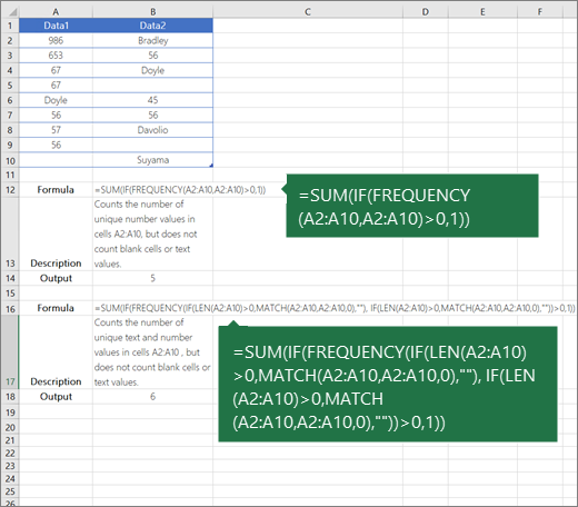
This formula is more complicated than a similar formula that uses FREQUENCY to count unique numeric values because FREQUENCY doesn’t work with non-numeric values. As a result, a large part of the formula simply transforms the non-numeric data into numeric data that FREQUENCY can handle.
Working from the inside-out, the MATCH function is used to get the position of each item that appears in the data:
MATCH(B5:B14,B5:B14,0)
The result from MATCH is an array like this:
{1;1;1;4;4;6;6;6;9;9}
Because MATCH always returns the position of the first match, values that appear more than once in the data return the same position. For example, because «Jim» appears 3 times in the list, he shows up in this array 3 times as the number 1.
This array is fed into FREQUENCY as the data_array argument. The bins_array argument is constructed from this part of the formula:
ROW(B5:B14)-ROW(B5)+1)
which builds a sequential list of numbers for each value in the data:
{1;2;3;4;5;6;7;8;9;10}
At this point, FREQUENCY is configured like this:
FREQUENCY({1;1;1;4;4;6;6;6;9;9},{1;2;3;4;5;6;7;8;9;10})
FREQUENCY returns an array of numbers that indicate a count for each number in the data array, organized by bin. When a number has already been counted, FREQUENCY will return zero. This is a key feature in the operation of this formula. The result from FREQUENCY is an array like this:
{3;0;0;2;0;3;0;0;2;0;0} // output from FREQUENCY
Note: FREQUENCY always returns an array with one more item than the bins_array.
We can now rewrite the formula like this:
=SUMPRODUCT(--({3;0;0;2;0;3;0;0;2;0;0}>0))
Next, we check for values greater than zero (>0), which converts the numbers to TRUE or FALSE, then use a double-negative (—) to convert the TRUE and FALSE values to 1s and 0s. Now we have:
=SUMPRODUCT({1;0;0;1;0;1;0;0;1;0;0})
Finally, SUMPRODUCT simply adds the numbers up and returns the total, which in this case is 4.
Handling blank cells
Empty cells in the range will cause the formula to return an #N/A error. To handle empty cells, you can use a more complicated array formula that uses the IF function to filter out blank values:
{=SUM(IF(FREQUENCY(IF(data<>"", MATCH(data,data,0)),ROW(data)-ROW(data.firstcell)+1),1))}
Note: adding IF makes this into an array formula that requires control-shift-enter.
For more information, see this page.
From Mike Givin’s excellent book on array formulas, Control-Shift-Enter.
UNIQUE function in Excel 365
In Excel 365, the UNIQUE function provides a better, more elegant way to list unique values and count unique values. These formulas can be adapted to apply logical criteria.
A pivot table is also an excellent way to list and count unique values.
Count unique values among duplicates
Excel for Microsoft 365 Excel for Microsoft 365 for Mac Excel for the web Excel 2021 Excel 2021 for Mac Excel 2019 Excel 2019 for Mac Excel 2016 Excel 2016 for Mac Excel 2013 Excel 2010 Excel 2007 Excel for Mac 2011 More…Less
Let’s say you want to find out how many unique values exist in a range that contains duplicate values. For example, if a column contains:
-
The values 5, 6, 7, and 6, the result is three unique values — 5 , 6 and 7.
-
The values «Bradley», «Doyle», «Doyle», «Doyle», the result is two unique values — «Bradley» and «Doyle».
There are several ways to count unique values among duplicates.
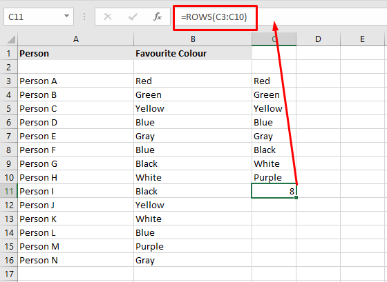
You can use the Advanced Filter dialog box to extract the unique values from a column of data and paste them to a new location. Then you can use the ROWS function to count the number of items in the new range.
-
Select the range of cells, or make sure the active cell is in a table.
Make sure the range of cells has a column heading.
-
On the Data tab, in the Sort & Filter group, click Advanced.
The Advanced Filter dialog box appears.
-
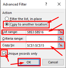
Click Copy to another location.
-
In the Copy to box, enter a cell reference.
Alternatively, click Collapse Dialog
 to temporarily hide the dialog box, select a cell on the worksheet, and then press Expand Dialog .
 -
Select the Unique records only check box, and click OK.
The unique values from the selected range are copied to the new location beginning with the cell you specified in the Copy to box.
-
In the blank cell below the last cell in the range, enter the ROWS function. Use the range of unique values that you just copied as the argument, excluding the column heading. For example, if the range of unique values is B2:B45, you enter =ROWS(B2:B45).
 to temporarily hide the dialog box, select a cell on the worksheet, and then press Expand Dialog
  .
.Use a combination of the IF, SUM, FREQUENCY, MATCH, and LEN functions to do this task:
-
Assign a value of 1 to each true condition by using the IF function.
-
Add the total by using the SUM function.
-
Count the number of unique values by using the FREQUENCY function. The FREQUENCY function ignores text and zero values. For the first occurrence of a specific value, this function returns a number equal to the number of occurrences of that value. For each occurrence of that same value after the first, this function returns a zero.
-
Return the position of a text value in a range by using the MATCH function. This value returned is then used as an argument to the FREQUENCY function so that the corresponding text values can be evaluated.
-
Find blank cells by using the LEN function. Blank cells have a length of 0.
Notes:
-
The formulas in this example must be entered as array formulas. If you have a current version of Microsoft 365, then you can simply enter the formula in the top-left-cell of the output range, then press ENTER to confirm the formula as a dynamic array formula. Otherwise, the formula must be entered as a legacy array formula by first selecting the output range, entering the formula in the top-left-cell of the output range, and then pressing CTRL+SHIFT+ENTER to confirm it. Excel inserts curly brackets at the beginning and end of the formula for you. For more information on array formulas, see Guidelines and examples of array formulas.
-
To see a function evaluated step by step, select the cell containing the formula, and then on the Formulas tab, in the Formula Auditing group, click Evaluate Formula.
-
The FREQUENCY function calculates how often values occur within a range of values, and then returns a vertical array of numbers. For example, use FREQUENCY to count the number of test scores that fall within ranges of scores. Because this function returns an array, it must be entered as an array formula.
-
The MATCH function searches for a specified item in a range of cells, and then returns the relative position of that item in the range. For example, if the range A1:A3 contains the values 5, 25, and 38, the formula =MATCH(25,A1:A3,0) returns the number 2, because 25 is the second item in the range.
-
The LEN function returns the number of characters in a text string.
-
The SUM function adds all the numbers that you specify as arguments. Each argument can be a range, a cell reference, an array, a constant, a formula, or the result from another function. For example, SUM(A1:A5) adds all the numbers that are contained in cells A1 through A5.
-
The IF function returns one value if a condition you specify evaluates to TRUE, and another value if that condition evaluates to FALSE.
Need more help?
You can always ask an expert in the Excel Tech Community or get support in the Answers community.
See Also
Filter for unique values or remove duplicate values
Need more help?
Want more options?
Explore subscription benefits, browse training courses, learn how to secure your device, and more.
Communities help you ask and answer questions, give feedback, and hear from experts with rich knowledge.
Well we have counted unique values using COUNTIF and SUMPRODUCT function. Although that method is easy but that is slow when data is large. In this article, we will learn how to count unique text values in excel with a faster formula
Generic formula to count unique text values in excel
Range : The range from which you want to get unique values.
firstCell in range: It is the reference of the first cell in range. If range is A2:A10 then it is A2.
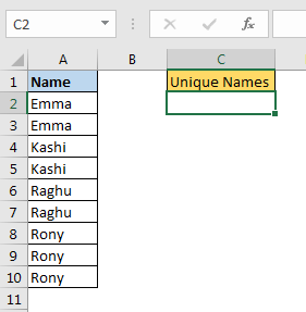
Let’s see an example to make things clear.
Example: Count Unique Text Values Excel
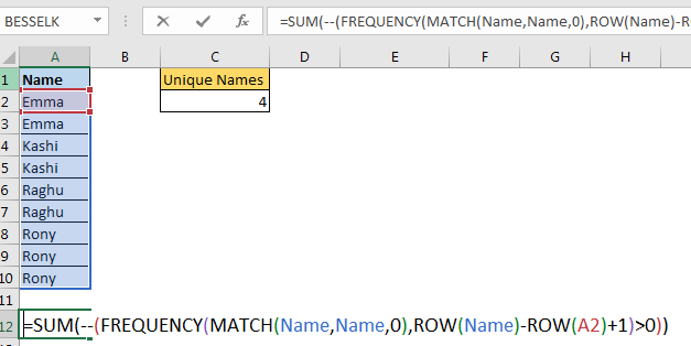
In an excel sheet, I have this data of names in range A2:A10. I want to get count of unique names from the given range.
Apply above generic formula here to count unique text in excel range A2:A10. I have named A2:A10 as names.
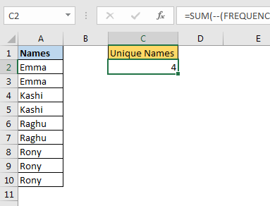
This returns the total count of unique texts in range A2:A10.
How it works?
Let’s solve it from inside.
MATCH(names,names,0): this part will return the first location of each value in range A2:A10 (names) as per MATCH’s property.
{1;1;3;3;5;5;7;7;7}.
Next ROW(A2:A19): This returns the row number of each cell in range A2:A10.
{2;3;4;5;6;7;8;9;10}
ROW(names)-ROW(A2): Now we subtract the first row number from each row number. This returns the an array of serial number starting from 0.
{0;1;2;3;4;5;6;7;8}
Since we want to have serial number starting from 1, we add 1 to it.
ROW(names)-ROW(A2)+1. This gives us an array of serial number starting from 1.
{1;2;3;4;5;6;7;8;9}
This will help us in getting unique count on condition.
Now we have:
FREQUENCY({1;1;3;3;5;5;7;7;7},{1;2;3;4;5;6;7;8;9}).
This returns the frequency of each number in given array.{2;0;2;0;2;0;3;0;0;0}
Here each positive number indicated occurrence of unique value when criteria is met. We need to count values greater than 0 in this array. For that we check it by >0. This will return TRUE and FALSE. We convert true false using — (double binary operator).
SUM(—({2;0;2;0;2;0;3;0;0;0})>0) this translates toSUM({1;0;1;0;1;0;1;0;0;0})
And finally we get the unique count of names in range on criteria as 4.
How to count unique text in range with blank cells?
The problem with above formula is that when you have blank cell in range, it will pop #N/A error. To tackle this we need to put a condition to check blank cells.
This will give correct output. Here we have encapsulated MATCH with IF function. You can read the full explanation in article How To Count Unique Values in Excel With Multiple Criteria?
So yeah guys, this how you can get unique text count in excel. Let me know if you have any doubts regarding this or any other advance excel/vba topic. The comments section is open for you.
Download file:
Related Articles:
How To Count Unique Values in Excel With Criteria
Excel Formula to Extract Unique Values From a List
Count Unique Values In Excel
Popular Articles:
The VLOOKUP Function in Excel
COUNTIF in Excel 2016
How to Use SUMIF Function in Excel
It might be challenging to work with a lot of data in Excel. Several repetitions of some values are possible. To improve your accuracy, you might need to consider numerous data entries when conducting any function. To organize the data or even to get statistics from it, you will also need to count the values. Manually counting the values would be extremely difficult with enormous amounts of data. It might be particularly difficult to keep track of distinct or unique values. Excel offers a variety of methods for counting different and unique data.
How to count unique text values in excel online, 2016 and 2019
Let’s look at how to count unique data in Excel first.
Using SUM, IF and Count functions in excel
Excel functions can be used to solve any operations at any time. To count unique values in Excel in this situation, combine the SUM, IF, and COUNTIF functions.
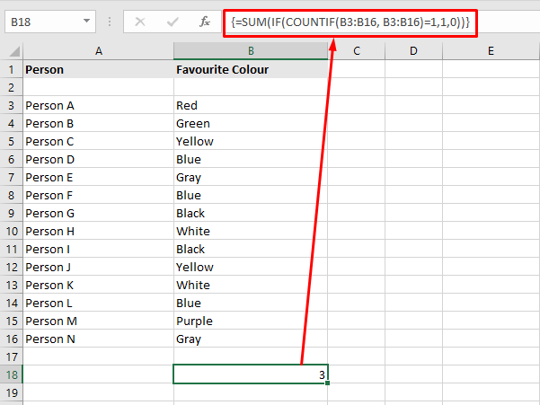
1.Enter the formula =SUM(IF(COUNTIF(range, range)=1,1,0)) in the desired cell to count unique values. The initial cell and the final cell are indicated by the range.The count values in this array formula are kept in a separate array. Make careful to use Ctrl+Shift+Enter after entering the formula because this is an array formula. Also take note that curly braces will be added automatically at the end of the formula when you enter it. But don’t manually enter them.
2.Think of the case from above. Enter the formula in the target cell to determine the distinct values in the provided Excel sheet.
3.Enter the cells containing the elements whose unique value is to be sought in place of range. The stated pieces are housed in cells B3 to B16 here. Thus, the equation is:=SUM(IF(COUNTIF(B3:B16, B3:B16)=1,1,0))
4.Press Ctrl+Shift+Enter to continue. This displays the number of distinct values within the chosen range. The number of unique values is 3.
1.Text and numbers may be combined in some tables and workbooks.
2.In these circumstances, you can modify the aforementioned function to find the distinct text values in Excel.In the target cell, type =SUM(IF(ISTEXT(range)*COUNTIF(range,range)=1,1,0)) and click Ctrl+Shift+Enter.
3.The start and end cells that contain the elements are indicated by the range.To determine the specific text values, we have added the ISTEXT element to the generic formula.
4.The ISTEXT method returns 1 and counts the value in an array if the value is a text. It returns 0 if the cell has a non-text value.The functionality is comparable to the widely used formula above.
Note: This above written article is an attempt to show you how to count unique text values in excel online, 2016 and 2019, in both windows and mac.You just need to have a little understanding of how and which way things work and you are good to go. With having this basic knowledge or information of how to use it, you can also access and use different other options on excel or spreadsheet. Also, it is very similar to Word or Document. So, in a way, if you learn one thing, like Excel, you can automatically learn how to use Word as well because both of them are very similar in so many ways. If you want to know more about WPS Office, you can download WPS Office to access, Word, Excel, PowerPoint for free.
Home > Microsoft Excel > How to Count Unique Values in Excel? 3 Easy Ways to Count Unique and Distinct Values
(Note: This guide on how to freeze rows in Excel is suitable for all Excel versions including Office 365)
Working with large amounts of data in Excel can be quite difficult. Some values may be repeated more than once. You might have to take into account multiple entries of data while performing any function to upgrade your accuracy. You will also need to count the values to organize or even acquire statistics from the data.
With large data, it would be nearly impossible to count the values manually. Especially, keeping a track of unique or distinct values can be quite arduous. Fortunately in Excel, there are many ways to count unique and distinct values.
You’ll Learn:
- Unique and Distinct Values
- How to Count Unique Values in Excel
- Using SUM, IF, and COUNTIF Functions
- Count Unique Text Values in Excel
- Count Unique Numeric Values in Excel
- Using SUM, IF, and COUNTIF Functions
- How to Count Distinct Values in Excel
- Using Filter Option
- Using SUM and COUNTIF functions
First, let us understand the difference between Unique and Distinct Values.
Unique and Distinct Values
Data can be repeated or unrepeated. These unrepeated data are of two types. They are called unique data and distinct data.
Unique data are those which occur in the dataset only once.
Whereas, distinct data include the duplicate values but count them only once.
I will explain unique and distinct data with an example for better understanding.
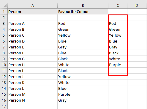
Consider an example, where column A has the list of people and column B lists their favorite colors.

In this, red, green, and purple colors occur only once, so they are called unique elements. Therefore the unique elements count is 3
Whereas, there are 8 distinct elements. That is the colors, though repeated are counted once. The colors are red, green, yellow, blue, white, black, gray, and purple. So, the distinct value count is 8.

In this guide, I will show you how to count unique and distinct values in Excel.
Let’s dive in.
How to Count Unique Values in Excel
First, let us see how to count unique values in excel.
Using SUM, IF, and COUNTIF Functions
In Excel, functions are always available to solve any operations. In this case, you can use a combination of SUM, IF and COUNTIF functions to count unique values in Excel.
To count unique values, enter the formula =SUM(IF(COUNTIF(range, range)=1,1,0)) in the desired cell. The range denotes the starting cell and the ending cell.
This is an array formula where the count values are stored in a new array. Since this is an array formula, make sure you press Ctrl+Shift+Enter after entering the formula. Also, note that when you enter the formula, curly braces will automatically populate at the end of them. But, do not enter them manually.
Consider the above example. To calculate the unique values in the given Excel sheet, enter the formula in the destination cell.
In the place of range, enter the cells which contain the elements whose unique value is to be found. Here, cells B3 to B16 house the said elements. So the formula becomes:
=SUM(IF(COUNTIF(B3:B16, B3:B16)=1,1,0))
Now, press Ctrl+Shift +Enter. This gives the count of unique values in the selected range. The unique value count is 3.
Simple, right? Now, let me explain how this formula gives the unique values in 3 simple steps.
- The COUNTIF function counts the number of unique values in the given range B3 to B16. That is the number of times the value is repeated in the range. These counted values are stored in an array. So, the array becomes [1,1,2,3,2,3,2,2,2,2,2,3,1,2]
- Then the IF function keeps the unique values(=1) and replaces anything other than 1 with 0. So the array becomes [1,1,0,0,0,0,0,0,0,0,0,0,1,0]
- Now finally, the SUM function adds the unique value and returns the value 3.
There are two additional cases while using the SUM, IF, and COUNTIF functions. You can use them to find either unique text values or numeric values in Excel.
Count Unique Text Values in Excel
In some tables and worksheets, some texts might be intertwined with numbers. In such cases, you can use the above-mentioned function with a little modification to find the unique text values in Excel.
Enter the formula =SUM(IF(ISTEXT(range)*COUNTIF(range,range)=1,1,0)) in the destination cell and press Ctrl+Shift+Enter. The range denotes the start and end cells that house the elements.
From the general formula, we have added the ISTEXT element to find the unique text values. If the value is a text, the ISTEXT function returns 1 and the value is counted in an array. If the cell houses a non-text value, it returns zero.
The functionality is also similar to the above common formula.
Count Unique Numeric values in Excel
This is a vice versa to the above-mentioned case. In case you only want to count unique numeric values intertwined with texts, you can use the below formula.
Enter the formula =SUM(IF(ISNUMBER(range)*COUNTIF(range,range)=1,1,0)) in the desired cell. The range denotes the start and end cells that hold the values.
Here, the ISNUMBER function returns 1 for numeric values and ignores other values. This function’s working is also similar to the above-mentioned case.
Note: In Excel, date and time are counted as numbers, so they are also counted.
We have seen how to count unique values in excel, we can also count distinct values by using the methods below.
How to Count Distinct Values in Excel
In Excel, there are two easy methods to find the number of distinct values.
Using Filter Option
This is an easy and simple method in Excel which gives you the unique values in your data. In this method, you can use the Filter option to pick out the distinct values. This option filters the elements to another row. then, you can use the ROWS function to find out the number of unique elements.
To find the unique rows using the Filter option, first select the rows/columns which have the duplicate elements.
Then, go to Data > Sort & Filter and click on Advanced.

The Advanced Filter dialog box appears.
Specify the List range: i.e select the cells you need to apply the filter to. You can enter them manually, or click on the Collapse button ![]() , select the area and click Expand .
, select the area and click Expand .
First, select the Copy to another location. This copied the unique elements onto a new column.
Now, use the collapse and expand button to select the rows you want the unique elements to be copied.
Finally, check Unique records only. And click OK.
Thus the distinct elements are copied onto a new row.
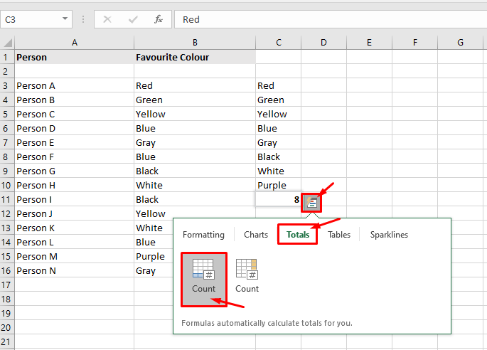
To calculate the row count, you can select the columns and click on Quick analysis or Ctrl + Q. Select Totals and click on Row Count. This will give you the row count right below the unique elements.
Or, you can use the function =ROWS(a:b), where a and b are the starting and ending cells respectively.
Note: If you click on Filter the list, in-place, the selected values will be replaced in the same column.
Using SUM and COUNTIF functions
You can use the SUM and COUNTIF functions to calculate the distinct values in Excel. In this case, we will inverse the COUNTIF function to arrive at distinct values.
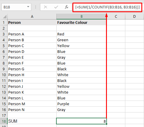
To count distinct values in excel, first enter the formula =SUM(1/COUNTIF(range, range)) in the desired cell. The range specifies the starting cell and ending cell separated by a colon. This is an array function, so press Ctrl+Shift+Enter to apply the formula.

Alternatively, you can also use the formula =SUMPRODUCT(1/COUNTIF(range, range)) in the desired cell to count distinct values. This is not an array function, so pressing Enter is sufficient to apply the formula.
Consider the same above-mentioned example. To count the distinct values, enter the formula =SUM(1/COUNTIF(B3:B16, B3:B16)) in the destination cell. Here, the range is B3:B16, so the values in cells B3 to B16 are taken into account.
First, the COUNTIF function counts the number of times the values occur in the given range. This value is stored in an array. Then, this value is divided by 1. So, if a value occurs twice, the value after dividing by 1 will be 0.5. Now, the SUM or SUMPRODUCT function adds up the fractional values and returns the result which is equal to the count of distinct values in the range.
Note: Similarly, you can also tweak the formulae a little to find distinct text values or distinct numeric values.
To find distinct text values: =SUM(IF(ISTEXT(range),1/COUNTIF(range, range),””))
To find distinct text values: =SUM(IF(ISNUMBER(range),1/COUNTIF(range, range),””))
Closing Thoughts
Finding the unique and distinct elements in a large dataset can be used to determine the statistics or probability of the data.
In this guide, we saw how to count unique and distinct values in Excel. Based on your specifications and preferences, you can either find the count of unique or distinct values.
If you need more high-quality Excel guides, please check out our free Excel resources center.
Simon Sez IT has been teaching Excel for over ten years. For a low, monthly fee you can get access to 100+ IT training courses. Click here for advanced Excel courses with in-depth training modules.
Simon Calder

Chris “Simon” Calder was working as a Project Manager in IT for one of Los Angeles’ most prestigious cultural institutions, LACMA.He taught himself to use Microsoft Project from a giant textbook and hated every moment of it. Online learning was in its infancy then, but he spotted an opportunity and made an online MS Project course — the rest, as they say, is history!
We can count unique text values in a range by using a combination of FREQUENCY, MATCH, ROW and SUMPRODUCT functions. We can also achieve the same result with the COUNTIF function. The steps below will walk through the process.
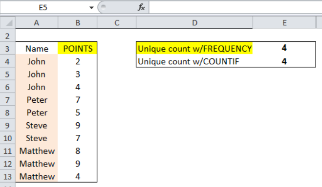 Figure 1: Result of Count of Unique Text Values in a Range
General formula
=SUMPRODUCT(--(FREQUENCY(MATCH(txt,txt,0),ROW(txt)-ROW(txt.firstcell+1)>0))
”txt” is the range containing the text or names
Formula
=SUMPRODUCT(--(FREQUENCY(MATCH(A4:A13,A4:A13,0),ROW(A4:A13)-ROW(A4)+1)>0))
Setting up the Data
We will set up the table as shown in figure 2 with hypothetical players who have scored some points. Now, we have players whose names have appeared more than once. Our intention is to count the number of unique names that appear.
- We will input the names in range A4:A13
- The points will be placed in Column B
- Cell E3 and Cell E4 will contain the results by applying the FREQUENCY and COUNTIF functions respectively
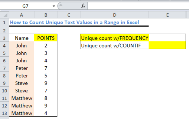 Figure 2: Setting up the Data
Applying the Frequency Function
- We will insert the formula below into Cell E3
=SUMPRODUCT(--(FREQUENCY(MATCH(A4:A13,A4:A13,0),ROW(A4:A13)-ROW(A4)+1)>0))
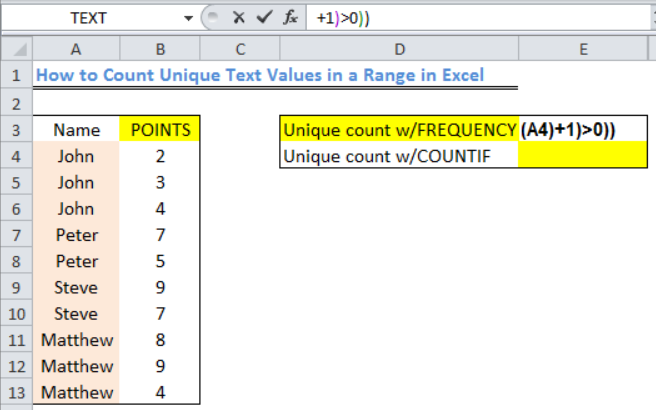 Figure 3: How to Count Unique Text Values in a Range
- We will press the enter key
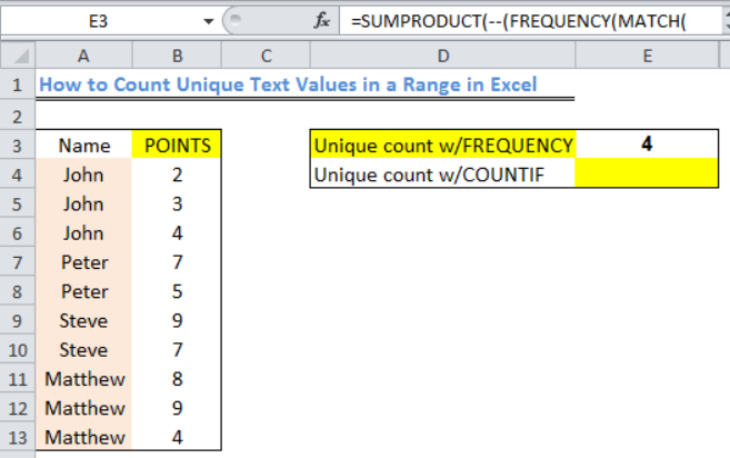 Figure 4: Result of Unique Text Values in the Range
Applying the COUNTIF Function
- We will insert the formula below into Cell E4
=SUMPRODUCT(1/COUNTIF(A4:A13,A4:A13))
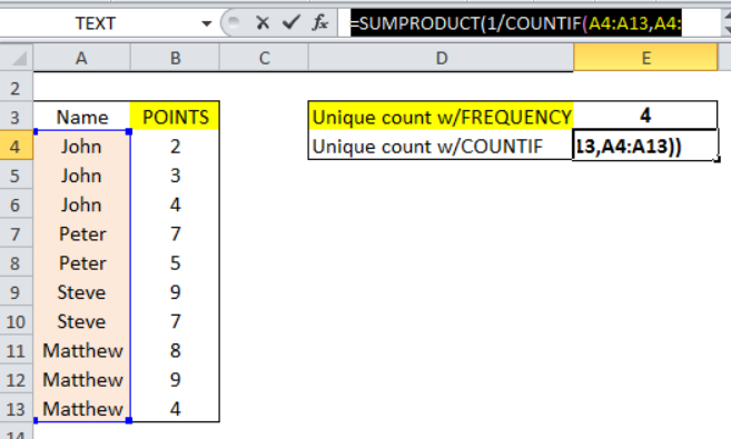 Figure 5: How to Count Unique Text Values in a Range with the COUNTIF function
- We will press the enter key
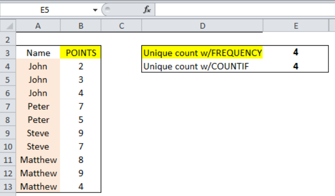 Figure 6: Result of Count of Unique Text Values in a Range
Explanation
=SUMPRODUCT(--(FREQUENCY(MATCH(A4:A13,A4:A13,0),ROW(A4:A13)-ROW(A4)+1)>0))
- MATCH Function
This function gets the position of each name in the range. MATCH only returns the position of the first match in the range, as a result, any name that appears more than once will bear the same number so that the returned array of this example looks like this:
{1;1;1;4;4;6;6;8;8;8}
- ROW Function
ROW(A4:A13)-ROW(A4)+1
The argument above is used to build a straight and sequential array. This is achieved by using the row number of each item in the range and the first item in the range. The returned array will look like this:
{1;2;3;4;5;6;7;8;9;10}
- FREQUENCY Function
The FREQUENCY function does not work with non-numeric data; hence, the bulk of the formula will convert the data into numeric data that FREQUENCY works with.
The FREQUENCY function uses the array supplied by MATCH and that supplied by ROW.
The FREQUENCY function will return an array of values that shows the count for every value that is present in the array. FREQUENCY will return zero for any number that repeats itself in the array. The resultant array will look like this:
{3;0;0;2;0;2;0;3;0;0;0}
- SUMPRODUCT Function
The returned array from FREQUENCY is evaluated by TRUE or FALSE to know if the numbers are greater than zero. Afterward, TRUE values are returned as 1 and FALSE as 0. The resultant array in SUMPRODUCT will look like this:
{1;0;0;1;0;1;0;1;0;0;0}
SUMPRODUCT then sums the values and the result is 4 as shown.
Instant Connection to an Expert through our Excelchat Service
Most of the time, the problem you will need to solve will be more complex than a simple application of a formula or function. If you want to save hours of research and frustration, try our live Excelchat service! Our Excel Experts are available 24/7 to answer any Excel question you may have. We guarantee a connection within 30 seconds and a customized solution within 20 minutes.
Let’s say you have a list of values where each value is entered more than once.
And now…
You want to count unique values from that list so that you can get the actual numbers of values that are there.
For this, you need to use a method that will count value only one time and ignore it’s all the other occurrences in the list.
In Excel, you can use different methods to get a count of unique values. It depends that which type of values you have so that you can use the best method for it.
In today’s post, I’d like to share with you 6 different methods to count unique values and use these methods according to the type of values you have.
data.xlsx
Advanced Filter to Get a Count of Unique Values
Using an advanced filter is one of the easiest ways to check the count of unique values and you don’t even need complex formulas. Here we have a list of names and from this list, you need to count the number of unique names.

Following are the steps you need to follow to get the unique values:
- First of all, select any of the cells from the list.
- After that, go to Data Tab ➜ Sort & Filter ➜ Click on Advanced.
- Once you click on it, you will get a pop-up window to apply advanced filters.
- Now from this window, select “Copy to another location”.
- In “Copy to”, select a blank cell where you want to paste unique values.
- Now, tick mark “Unique Records Only” and click OK.
- At this point, you have a list of unique values.
- Now, go to the cell below the last cell of the list and insert the following formula and hit enter.


=COUNTA(B2:B10)It will return the count of unique values from that list of names.

Now you have a list of unique values and count as well. This method is simple and easy to follow as you don’t need to write complex formulas for this.
Combination of SUM and COUNTIF to Count Unique Values
If you want to find the count of unique values in a single cell without extracting a separate list, then you can use a combination of SUM and COUNTIF.
In this method, you just have to refer to the list of the values and the formula will return the number of unique values. This is an array formula, so you need to enter it as an array, and while entering it use Ctrl + Shift + Enter.
And the formula is:
=SUM(1/COUNTIF(A2:A17,A2:A17))When you enter this formula as an array it will look something like this.
{=SUM(1/COUNTIF(A2:A17,A2:A17))}
How it Works
To understand this formula you need to break it down into three parts and just remember that we have entered this formula as an array and there is a total of 16 values in this list, not unique but total.
Ok, so look.
In the first part, you have used COUNIF to count the number of each value from 16 and here COUNTIF returns values like the below.

In the second part, you have divided all the values by 1 which returns a value like this.

Let’s say if a value is there in the list twice, then it will return 0.5 for both of the values so that in the end when you sum it, it becomes 1 and if a value is there three times it will return 0.333 for each.
And, in the third part, you have simply used the SUM function to sum all those values and you have a count of unique values.
This formula is quite powerful and it can help you to get the count in a single cell.
Use SUMPRODUCT + COUNTIF to Get a Number of Unique Values from a List
In the last method, you used the SUM and COUNTIF methods. But, you can also use SUMPRODUCT instead of SUM.
And, when you use SUMPRODUCT, you don’t need to enter a formula as an array. Just edit the cell and enter the below formula.
=SUMPRODUCT(1/COUNTIF(A2:A17,A2:A17))When you enter this formula as an array it will look something like this.
{=SUMPRODUCT(1/COUNTIF(A2:A17,A2:A17))}
How it Works
This formula exactly works in the same way as you have learned in the above method, the difference is just that you have used SUMPRODUCT instead of SUM.
And SUMPRODUCT can take an array without using Ctrl + Shift + Enter.
Count Only Unique Text Values from a List
Now, let’s say you have a list of names in which you also have mobile numbers and you want to count unique values just from text values. So in this case, you can use the below formula:
=SUM(IF(ISTEXT(A2:A17),1/COUNTIF(A2:A17, A2:A17),””))And when you enter this formula as an array.
{=SUM(IF(ISTEXT(A2:A17),1/COUNTIF(A2:A17, A2:A17),””))}
How it Works
In this method, you have used the IF function and ISTEXT. ISTEXT first verifies whether all the values are text or not and return TRUE if a value is text.

After that, IF applies COUNTIF on all the text values where you have TRUE and other values remain blank.

And in the end, SUM returns the sum of all the unique values which are text and you get the count of unique text values this way.
Get Count of Unique Numbers from a List
And if you just want to count unique numbers from a list of values then you can use the below formula.
=SUM(IF(ISNUMBER(A2:A17),1/COUNTIF(A2:A17, A2:A17),””))Enter this formula as an array.
{=SUM(IF(ISNUMBER(A2:A17),1/COUNTIF(A2:A17, A2:A17),””))}
How it works
In this method, you have used the IF function and ISNUMBER. ISNUMBER first verifies that all the values are numeric or not and return TRUE if a value is a number.
After that, IF applies COUNTIF on all the numeric values where you have TRUE and other values remain blank.
And in the end, SUM returns the sum of all the unique values which are numbers and you get the count of unique numbers this way.
Count Unique Values with a UDF
Here I have VBA (UDF) which can help you to count unique values without using any kind of formula.
Function CountUnique(ListRange As Range) As Integer
Dim CellValue As Variant
Dim UniqueValues As New Collection
Application.Volatile
On Error Resume Next
For Each CellValue In ListRange
UniqueValues.Add CellValue, CStr(CellValue) ' add the unique item
Next
CountUnique = UniqueValues.Count
End Function
Enter this function in your VBE by inserting a new module and after that go to your worksheet and insert the following formula.
=CountUnique(range)
Download Sample File
- Ready
Conclusion
Counting unique values can be useful for you while working with large datasets.
The name list which you have used here had duplicate names and after calculating unique numbers, we get that there are 10 unique names in the list.
Well, all the methods which you have learned here are useful in different situations and you can use anyone from those which you think is a perfect fit for you.
If you ask me, advanced filter and SUMPRODUCT are my favorite methods, but now you need to tell me:
Which one is your favorite?
Please share your views with me in the comment section, I’d love to hear from you and don’t forget to share this tip with your friends.
Let’s consider we have a long list of duplicate values in a range and our objective is to count only the unique occurrences of each value.
Though this can be a very common requirement in many scenarios but excel doesn’t have any single formula that can directly help us to count unique values in excel inside a range.
In today’s post, we will see 5 different ways of counting unique values in excel.
But, before starting let’s make our goal clear.

By looking at the above image, we can clearly see that what we mean by counting unique value in excel.
Method – 1: Using SumProduct and CountIF Formula:
The simplest and easiest way to count distinct values in excel is to use SumProduct and CountIF formula.
Following is the generic formula that you can use:
=SUMPRODUCT(1/COUNTIF(data,data))
‘data’ – data represents the range that contains the values

Let’s See How This Formula Works:
This formula consists of two functions combined together. Let’s first understand the role of inner CountIF function.
The CountIF function looks inside the data range (B2:B9) and counts the number of times each value appears in data range.
The result is an array of numbers and in our example it might look something like this: {2;2;3;3;3;2;2;1}.
Next, the results of CountIF formula are used as a divisor with 1 as numerator. This modifies the result of CountIF formula such that; values that only appear once in the array become 1 and the numbers corresponding to duplicate values become fractions corresponding to the multiple.
This means that, if a value appears 4 times in the range then its value will become as 1/4 = 0.25 and value that is present only once will become 1/1 = 1
Finally, the SumProduct formula adds up all the elements in the array and returns the final result.
Read these articles for more details on CountIF Function or SumProduct Function.
The Catch:
This formula woks nicely on a continuous set of values in a range, however if your values contain empty cells, then this formula fails. In such cases the formula throws a ‘divide by zero’ error.
Because, CountIF function generates a ‘0’ for each blank cell and when 1 is divided by 0 it returns a divide by zero error.

To fix this, you can use the following variant of the above formula that ignores the blank cells:
=SUMPRODUCT(((data<>"")/COUNTIF(data , data &"")))
‘data’ – data represents the range that contains the values

Method – 2: Using SUM, FREQUENCY AND MATCH Array Formula
The formula that we discussed above is good to be used for small ranges. As the range becomes bigger the SUMPRODUCT and COUNTIF formula will become slower and will eventually make your spreadsheets unresponsive while counting unique values inside a range.
So, for larger datasets, you may want to switch to a formula based on the FREQUENCY function.
The generic formula is as follows:
=SUM(IF(FREQUENCY(IF(data<>"", MATCH(data,data,0)),ROW(data)-ROW(firstcell)+1),1))
Here, ‘data’ represents the range that contains the values.
And ‘firstcell’ represents the first cell of the range.
Note: This is an array formula so, after writing the formula press ‘Control-Shift-Enter’ and the formula will get surrounded by curly braces as shown below.

Let’s Try To Understand How This Formula Works:
This formula uses Frequency function to count the unique values, but the problem here is that FREQUENCY function is only designed to work with numbers. So, here our first objective is to convert the values into a set of numbers.
Starting from inside, the MATCH function in this formula gives us the first occurrence or position number of each item that appears in the data range. If there are any values that are duplicate, then MATCH will return only the position of the first occurrence of that value in the data range.
After the MATCH function, there is an IF Statement. The reason IF function is required because MATCH will return a #N/A error for empty cells. So, we are excluding the empty cells with data <> "".
The resulting array contains a set of numbers combined with False for the blank cells. So, in our case the resulting array would be like:
{1;1;3;3;3;6;FALSE;6;9}
This array is fed to the FREQUENCY function which returns how often values occur within the set of data and finally the outer IF function sets each unique value to 1 and duplicate value to FALSE.
And the final result comes out to be 4.
Method – 3: Using PivotTable (Only works in Excel 2013 and above)
The integration of power pivot with excel (known as Data Model), has provided some powerful features to the users. Now pivot tables can also help you to get the distinct counts of unique values in excel.
To do this follow the below steps:
- Navigate to the ‘Insert’ option on the top ribbon and click the ‘PivotTable’ option.

- This will open a ‘PivotTable’ dialog, select the data range and check the checkbox that says ‘Add this data to Data Model’ and finally click ‘Ok’ button.

- Build the PivotTable by placing the column that contains data range ‘Values’ and in the ‘Rows’ quadrant as shown below.

- Doing this will show the total count including the duplicate values, however we only need to get the count of distinct values. So, right click over the Count column and select the ‘Value Field Settings’ option.

- Next, In the ‘Value Field Settings’ window, select the ‘Distinct Count’ option and click ‘Ok’ button.

- Doing this will fetch the distinct counts for the values and populate them in the PivotTable.

Method – 4: Using SUM and COUNTIF function
This is again an array formula to count distinct values in a range.
=SUM(IF(ISTEXT(range),1/COUNTIF(range, range), ""))
Here, ‘range’ represents the range that contains the values.
Note: This is an array formula so, after writing the formula press ‘Control-Shift-Enter’ and the formula will get surrounded by curly braces as shown below.

Let’s See How This Formula Works:
In this formula, we have used ISTEXT function. ISTEXT function returns a true for all the values that are text and false for other values.
If the value is a text value, then the COUNTIF function executes and looks inside the data range (B2:B9) and counts the number of times that each value appears in data range.
After this, the result of CountIF function are used as a divisor with 1 as the numerator (same as in first method). This means that, if a value appears 4 times in the range its value will become as 1/4 = 0.25 and when the value is present only once then it becomes 1/1 = 1
Finally, the SUM function computes the sum of all the values and returns the result.
Method 5 – COUNTUNIQUE User Defined Function:
If none of the above options work for you, then you can create your own user defined function (UDF) that can count unique values in excel for you.
Below is the code to write your own UDF that does the same:
Function COUNTUNIQUE(DataRange As Range, CountBlanks As Boolean) As Integer
Dim CellContent As Variant
Dim UniqueValues As New Collection
Application.Volatile
On Error Resume Next
For Each CellContent In DataRange
If CountBlanks = True Or IsEmpty(CellContent) = False Then
UniqueValues.Add CellContent, CStr(CellContent)
End If
Next
COUNTUNIQUE = UniqueValues.Count
End Function
To embed this function in Excel use the following steps:
- Press Alt + F11 key on the Excel, this will open the VBA window.
- On the VBA Window, right click over the ‘Microsoft Excel Objects’ > ‘Insert’ > ‘Module’.

- Clicking the ‘Module’ will open a new module in the Excel. Paste the UDF code in the module window as shown below.

- Finally, save your spreadsheet and the formula is ready to use.
How to Use the UDF:
To use the UDF, you can simply type the UDF name ‘CountUnique’ like a normal excel function.
=COUNTUNIQUE(data_range, count_blanks)
‘data_range’ – represents the range that contains the values.
‘count_blanks’ – is a boolean parameter that can have two values true or false. If you set this parameter as true then it will count the blank rows as unique. By setting this parameter to false the UDF will exclude the blank rows.

So, these were all the methods that can help you to count unique value in excel. Do let us know your own methods or tricks to do the same.