
Locate hidden cells
Follow these steps:
-
Select the worksheet containing the hidden rows and columns that you need to locate, then access the Special feature with one of the following ways:
-
Press F5 > Special.
-
Press Ctrl+G > Special.
-
Or on the Home tab, in the Editing group, click Find & Select>Go To Special.
-
-
Under Select, click Visible cells only, and then click OK.

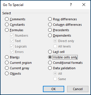
All visible cells are selected and the borders of rows and columns that are adjacent to hidden rows and columns will appear with a white border.
Note: Click anywhere on the worksheet to cancel the selection of the visible cells. If the hidden cells that you need to reveal are outside the visible worksheet area, use the scroll bars to move through the document until the hidden rows and columns that contain those cells are visible.
This feature is not available in Excel for the web.
Acts of mischief – that’s one word which comes into our mind when the spreadsheets we get have some ‘hidden’ agenda. Though it may be unintentional, it gets us into a grave problem when certain entries go hiding, especially when there is a formula involved. It makes us lose our precious time, leaving us scratching our heads on what went possibly wrong.
Also read: How to Hide Cells in MS Excel?
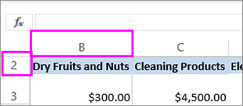
One might adopt all the troubleshooting techniques that one knows of, only to find out that the culprit lies not in the formula but hidden between the rows or the columns. Consider the following example in which column C is hidden between columns B & D.

In this article, we shall set out to explore how to unhide the hidden cells in the above data using each of the below techniques.
- The Conventional Right Click
- The Accelerator Way
Method 1 – The Conventional Right Click:
The mouse would be the weapon of choice in this technique, facilitating us with the oldest trick in the book – the RIGHT CLICK! One shall get started by selecting both the columns between which a column lies hidden. In this case, one shall select columns B to D as shown below.

The selection can be done by hovering the cursor & pulling it from wherever it is to the portion where the column names are indicated by letters. It is in this region that the cursor changes from a normal mouse pointer to a thick black arrow facing downwards as shown in the below image.

Now one shall click right on the top of the column at the letter ‘B’ & drag the cursor towards the right to column ‘D’. Once done, right-click anywhere within the selected region as done in the image below.

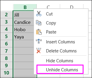
There shall be a right-click menu appearing with a list of options. Choose the Unhide option in the list & the hidden culprits would appear right in front of your eyes as shown below.

Method 2 – The Accelerator Way:
This technique is way simpler & relies more on the keyboard for successful execution. The first step of selecting the cells to unhide hidden cells remains the same as that of the previous method.

Once done, hit the ALT key on the keyboard followed by the letter keys O, C & U.
ALT + O + C + U
All these keys are to be pressed one after the other & not simultaneously. Doing the latter would only render this technique non-functional. It is also to be noted that the succeeding key is to be pressed after lifting the finger off the preceding key – to put in simple words, not similar to what one does with CTRL+C for copying or CTRL+V for pasting.
The moment the last key in the sequence, the letter key ‘U’ is hit, the hidden cells appear in a blink of an eye!

Both the techniques serve the purpose when the cells are also hidden horizontally along the rows, rather than vertically along the columns as given in the above examples.
Summary
Now we have reached the end of this article detailing how to unhide cells in MS Excel. Hope it has provided you with the sufficient information that you were looking for. Here is something that elaborates on How to Move a Column in MS Excel? Go on & read it to know further. There are also numerous other articles in QuickExcel that can come in handy for those who would like to constantly upgrade themselves in MS Excel. Cheers!
Learn several ways to do this
Updated on September 19, 2022
What to Know
- Hide a column: Select a cell in the column to hide, then press Ctrl+0. To unhide, select an adjacent column and press Ctrl+Shift+0.
- Hide a row: Select a cell in the row you want to hide, then press Ctrl+9. To unhide, select an adjacent column and press Ctrl+Shift+9.
- You can also use the right-click context menu and the format options on the Home tab to hide or unhide individual rows and columns.
You can hide columns and rows in Excel to make a cleaner worksheet without deleting data you might need later, although there is no way to hide individual cells. In this guide, we provide instructions for three ways to hide and unhide columns in Excel 2019, 2016, 2013, 2010, 2007, and Excel for Microsoft 365.
Hide Columns in Excel Using a Keyboard Shortcut
The keyboard key combination for hiding columns is Ctrl+0.
-
Click on a cell in the column you want to hide to make it the active cell.
-
Press and hold down the Ctrl key on the keyboard.
-
Press and release the 0 key without releasing the Ctrl key. The column containing the active cell should be hidden from view.
To hide multiple columns using the keyboard shortcut, highlight at least one cell in each column to be hidden, and then repeat steps two and three above.
Hide Columns Using the Context Menu
The options available in the context — or right-click menu — change depending upon the object selected when you open the menu. If the Hide option, as shown in the image below, is not available in the context menu it is likely that you didn’t select the entire column before right-clicking.
Hide a Single Column
-
Click the column header of the column you want to hide to select the entire column.
-
Right-click on the selected column to open the context menu.
-
Choose Hide. The selected column, the column letter, and any data in the column will be hidden from view.
Hide Adjacent Columns
-
In the column header, click and drag with the mouse pointer to highlight all three columns.
-
Right-click on the selected columns.
-
Choose Hide. The selected columns and column letters will be hidden from view.
When you hide columns and rows containing data, it does not delete the data, and you can still reference it in formulas and charts. Hidden formulas containing cell references will update if the data in the referenced cells changes.
Hide Separated Columns
-
In the column header click on the first column to be hidden.
-
Press and hold down the Ctrl key on the keyboard.
-
Continue to hold down the Ctrl key and click once on each additional column to be hidden to select them.
-
Release the Ctrl key.
-
In the column header, right-click on one of the selected columns and choose Hide. The selected columns and column letters will be hidden from view.
When hiding separate columns, if the mouse pointer is not over the column header when you click the right mouse button, the hide option will not be available.
Hide and Unhide Columns in Excel Using the Name Box
This method can be used to unhide any single column. In our example, we will be using column A.
-
Type the cell reference A1 into the Name Box.
-
Press the Enter key on the keyboard to select the hidden column.
-
Click on the Home tab of the ribbon.
-
Click on the Format icon on the ribbon to open the drop-down.
-
In the Visibility section of the menu, choose Hide & Unhide > Hide Columns or Unhide Column.
Unhide Columns Using a Keyboard Shortcut
The key combination for unhiding columns is Ctrl+Shift+0.
-
Type the cell reference A1 into the Name Box.
-
Press the Enter key on the keyboard to select the hidden column.
-
Press and hold down the Ctrl and the Shift keys on the keyboard.
-
Press and release the 0 key without releasing the Ctrl and Shift keys.
To unhide one or more columns, highlight at least one cell in the columns on either side of the hidden column(s) with the mouse pointer.
-
Click and drag with the mouse to highlight columns A to G.
-
Press and hold down the Ctrl and the Shift keys on the keyboard.
-
Press and release the 0 key without releasing the Ctrl and Shift keys. The hidden column(s) will become visible.
The Ctrl+Shift+0 keyboard shortcut might not work depending on the version of Windows you’re running, for reasons not explained by Microsoft. If this shortcut doesn’t work, use another method from the article.
Unhide Columns Using the Context Menu
As with the shortcut key method above, you must select at least one column on either side of a hidden column or columns to unhide them. For example, to unhide columns D, E, and G:
-
Hover the mouse pointer over column C in the column header. Click and drag with the mouse to highlight columns C to H to unhide all columns at one time.
-
Right-click on the selected columns and choose Unhide. The hidden column(s) will become visible.
Hide Rows Using Shortcut Keys
The keyboard key combination for hiding rows is Ctrl+9:
-
Click on a cell in the row you want to hide to make it the active cell.
-
Press and hold down the Ctrl key on the keyboard.
-
Press and release the 9 key without releasing the Ctrl key. The row containing the active cell should be hidden from view.
To hide multiple rows using the keyboard shortcut, highlight at least one cell in each row you want to hide, and then repeat steps two and three above.
Hide Rows Using the Context Menu
The options available in the context menu — or right-click — change depending upon the object selected when you open it. If the Hide option, as shown in the image above, is not available in the context menu it is because you probably didn’t select the entire row.
Hide a Single Row
-
Click on the row header for the row to be hidden to select the entire row.
-
Right-click on the selected row to open the context menu.
-
Choose Hide. The selected row, the row letter, and any data in the row will be hidden from view.
Hide Adjacent Rows
-
In the row header, click and drag with the mouse pointer to highlight all three rows.
-
Right-click on the selected rows and choose Hide. The selected rows will be hidden from view.
Hide Separated Rows
-
In the row header, click on the first row to be hidden.
-
Press and hold down the Ctrl key on the keyboard.
-
Continue to hold down the Ctrl key and click once on each additional row to be hidden to select them.
-
Right-click on one of the selected rows and choose Hide. The selected rows will be hidden from view.
Hide and Unhide Rows Using the Name Box
This method can be used to unhide any single row. In our example, we will be using row 1.
-
Type the cell reference A1 into the Name Box.
-
Press the Enter key on the keyboard to select the hidden row.
-
Click on the Home tab of the ribbon.
-
Click on the Format icon on the ribbon to open the drop-down menu.
-
In the Visibility section of the menu, choose Hide & Unhide > Hide Rows or Unhide Row.
Unhide Rows Using a Keyboard Shortcut
The key combination for unhiding rows is Ctrl+Shift+9.
Unhide Rows using Shortcut Keys and Name Box
-
Type the cell reference A1 into the Name Box.
-
Press the Enter key on the keyboard to select the hidden row.
-
Press and hold down the Ctrl and the Shift keys on the keyboard.
-
Press and hold down the Ctrl and the Shift keys on the keyboard. Row 1 will become visible.
Unhide Rows Using a Keyboard Shortcut
To unhide one or more rows, highlight at least one cell in the rows on either side of the hidden row(s) with the mouse pointer. For example, you want to unhide rows 2, 4, and 6.
-
To unhide all rows, click and drag with the mouse to highlight rows 1 to 7.
-
Press and hold down the Ctrl and the Shift keys on the keyboard.
-
Press and release the number 9 key without releasing the Ctrl and Shift keys. The hidden row(s) will become visible.
Unhide Rows Using the Context Menu
As with the shortcut key method above, you must select at least one row on either side of a hidden row or rows to unhide them. For example, to unhide rows 3, 4, and 6:
-
Hover the mouse pointer over row 2 in the row header.
-
Click and drag with the mouse to highlight rows 2 to 7 to unhide all rows at one time.
-
Right-click on the selected rows and choose Unhide. The hidden row(s) will become visible.
How to Move Columns in Excel
FAQ
-
How do I hide cells in Excel?
Select the cell or cells you want to hide, then select the Home tab > Cells > Format > Format Cells. In the Format Cells menu, select the Number tab > Custom (under Category) and type ;;; (three semicolons), then select OK.
-
How do I hide gridlines in Excel?
Select the Page Layout tab, then turn off the View checkbox under Gridlines.
-
How do I hide formulas in Excel?
Select the cells with formulas you want to hide > select the Hidden checkbox on the Protection tab > OK > Review > Protect Sheet. Next, verify that Protect worksheet and contents of locked cells is turned on, then select OK.
Thanks for letting us know!
Get the Latest Tech News Delivered Every Day
Subscribe
Содержание
- Unhide the first column or row in a worksheet
- How to hide and unhide rows in Excel
- How to hide rows in Excel
- Hide rows using the ribbon
- Hide rows using the right-click menu
- Excel shortcut to hide row
- How to unhide rows in Excel
- Unhide rows by using the ribbon
- Unhide rows using the context menu
- Unhide rows with a keyboard shortcut
- Show hidden rows by double-clicking
- How to unhide all rows in Excel
- How to unhide all cells in Excel
- How to unhide specific rows in Excel
- How to unhide top rows in Excel
- Tips and tricks for hiding and unhiding rows in Excel
- How to hide rows containing blank cells
- How to hide rows based on cell value
- Hide unused rows so that only working area is visible
- How to locate all hidden rows on a sheet
- How to copy visible rows in Excel
- Cannot unhide rows in Excel
- 1. The worksheet is protected
- 2. Row height is small, but not zero
- 3. Trouble unhiding the first row in Excel
- 4. Some rows are filtered out
Unhide the first column or row in a worksheet
If the first row (row 1) or column (column A) is not displayed in the worksheet, it is a little tricky to unhide it because there is no easy way to select that row or column. You can select the entire worksheet, and then unhide rows or columns ( Home tab, Cells group, Format button, Hide & Unhide command), but that displays all hidden rows and columns in your worksheet, which you may not want to do. Instead, you can use the Name box or the Go To command to select the first row and column.
To select the first hidden row or column on the worksheet, do one of the following:
In the Name Box next to the formula bar, type A1, and then press ENTER.
On the Home tab, in the Editing group, click Find & Select, and then click Go To. In the Reference box, type A1, and then click OK.
On the Home tab, in the Cells group, click Format.
Do one of the following:
Under Visibility, click Hide & Unhide, and then click Unhide Rows or Unhide Columns.
Under Cell Size, click Row Height or Column Width, and then in the Row Height or Column Width box, type the value that you want to use for the row height or column width.
Tip: The default height for rows is 15, and the default width for columns is 8.43.
If you don’t see the first column (column A) or row (row 1) in your worksheet, it might be hidden. Here’s how to unhide it. In this picture column A and row 1 are hidden.
To unhide column A, right-click the column B header or label and pick Unhide Columns.
To unhide row 1, right-click the row 2 header or label and pick Unhide Rows.
Tip: If you don’t see Unhide Columns or Unhide Rows, make sure you’re right-clicking inside the column or row label.
Источник
How to hide and unhide rows in Excel
 by Svetlana Cheusheva, updated on March 17, 2023
The tutorial shows three different ways to hide rows in your worksheets. It also explains how to show hidden rows in Excel and how to copy only visible rows.
If you want to prevent users from wandering into parts of a worksheet you don’t want them to see, then hide such rows from their view. This technique is often used to conceal sensitive data or formulas, but you may also wish to hide unused or unimportant areas to keep your users focused on relevant information.
On the other hand, when updating your own sheets or exploring inherited workbooks, you would certainly want to unhide all rows and columns to view all data and understand the dependencies. This article will teach you both options.
How to hide rows in Excel
As is the case with nearly all common tasks in Excel, there is more than one way to hide rows: by using the ribbon button, right-click menu, and keyboard shortcut.
Anyway, you begin with selecting the rows you’d like to hide:
- To select one row, click on its heading.
- To select multiple contiguous rows, drag across the row headings using the mouse. Or select the first row and hold down the Shift key while selecting the last row.
- To select non-contiguous rows, click the heading of the first row and hold down the Ctrl key while clicking the headings of other rows that you want to select.
With the rows selected, proceed with one of the following options.
Hide rows using the ribbon
If you enjoy working with the ribbon, you can hide rows in this way:
- Go to the Home tab >Cells group, and click the Format button.
- Under Visibility, point to Hide & Unhide, and then select Hide Rows.
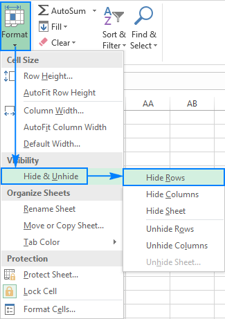
Alternatively, you can click Home tab >Format > Row Height… and type 0 in the Row Height box.
Either way, the selected rows will be hidden from view straight away.
In case you don’t want to bother remembering the location of the Hide command on the ribbon, you can access it from the context menu: right click the selected rows, and then click Hide. 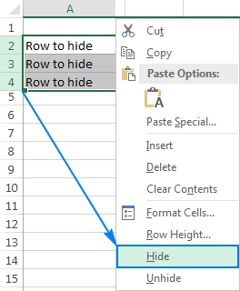
Excel shortcut to hide row
If you’d rather not take your hands off the keyboard, you can quickly hide the selected row(s) by pressing this shortcut: Ctrl + 9
How to unhide rows in Excel
As with hiding rows, Microsoft Excel provides a few different ways to unhide them. Which one to use is a matter of your personal preference. What makes the difference is the area you select to instruct Excel to unhide all hidden rows, only specific rows, or the first row in a sheet.
Unhide rows by using the ribbon
On the Home tab, in the Cells group, click the Format button, point to Hide & Unhide under Visibility, and then click Unhide Rows. 
You select a group of rows including the row above and below the row(s) you want to unhide, right-click the selection, and choose Unhide in the pop-up menu. This method works beautifully for unhiding a single hidden row as well as multiple rows.
For example, to show all hidden rows between rows 1 and 8, select this group of rows like shown in the screenshot below, right-click, and click Unhide: 
Unhide rows with a keyboard shortcut
Here is the Excel Unhide Rows shortcut: Ctrl + Shift + 9
Pressing this key combination (3 keys simultaneously) displays any hidden rows that intersect the selection.
Show hidden rows by double-clicking
In many situations, the fastest way to unhide rows in Excel is to double click them. The beauty of this method is that you don’t need to select anything. Simply hover your mouse over the hidden row headings, and when the mouse pointer turns into a split two-headed arrow, double click. That’s it! 
How to unhide all rows in Excel
In order to unhide all rows on a sheet, you need to select all rows. For this, you can either:
- Click the Select All button (a little triangle at the upper left corner of a sheet, in the intersection of the row and column headings):
- Press the Select All shortcut: Ctrl + A
Please note that in Microsoft Excel, this shortcut behaves differently in different situations. If the cursor is in an empty cell, the whole worksheet is selected. But if the cursor is in one of contiguous cells with data, only that group of cells is selected; to select all cells, press Ctrl+A one more time.
Once the entire sheet is selected, you can unhide all rows by doing one of the following:
- Press Ctrl + Shift + 9 (the fastest way).
- Select Unhide from the right-click menu (the easiest way that does not require remembering anything).
- On the Home tab, click Format >Unhide Rows (the traditional way).
How to unhide all cells in Excel
To unhide all rows and columns, select the whole sheet as explained above, and then press Ctrl + Shift + 9 to show hidden rows and Ctrl + Shift + 0 to show hidden columns.
How to unhide specific rows in Excel
Depending on which rows you want to unhide, select them as described below, and then apply one of the unhide options discussed above.
- To show one or several adjacent rows, select the row above and below the row(s) that you want to unhide.
- To unhide multiple non-adjacent rows, select all the rows between the first and last visible rows in the group.
For example, to unhide rows 3, 7, and 9, you select rows 2 — 10, and then use the ribbon, context menu or keyboard shortcut to unhide them.
How to unhide top rows in Excel
Hiding the first row in Excel is easy, you treat it just like any other row on a sheet. But when one or more top rows are hidden, how do you make them visible again, given that there is nothing above to select?
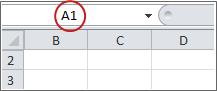
The clue is to select cell A1. For this, just type A1 in the Name Box, and press Enter. 
Alternatively, go to the Home tab > Editing group, click Find & Select, and then click Go To… . The Go To dialog window pops up, you type A1 in the Reference box, and click OK. 
With cell A1 selected, you can unhide the first hidden row in the usual way, by clicking Format > Unhide Rows on the ribbon, or choosing Unhide from the context menu, or pressing the unhide rows shortcut Ctrl + Shift + 9
Aside from this common approach, there is one more (and faster!) way to unhide first row in Excel. Simply hover over the hidden row heading, and when the mouse pointer turns into a split two-headed arrow, double click: 
Tips and tricks for hiding and unhiding rows in Excel
As you have just seen, hiding and showing rows in Excel is quick and straightforward. In some situations, however, even a simple task can become a challenge. Below you will find easy solutions to a few tricky problems.
How to hide rows containing blank cells
To hide rows that contain any blank cells, proceed with these steps:
- Select the range that contains empty cells you want to hide.
- On the Home tab, in the Editing group, click Find & Select >Go To Special.
- In the Go To Special dialog box, select the Blanks radio button, and click OK. This will select all empty cells in the range.
- Press Ctrl + 9 to hide the corresponding rows.
This method works well when you want to hide all rows that contain at least one blank cell, as shown in the screenshot below: ![]()
If you want to hide blank rows in Excel, i.e. the rows where all cells are blank, then use the COUNTBLANK formula explained in How to remove blank rows to identify such rows.
How to hide rows based on cell value
To hide and show rows based on a cell value in one or more columns, use the capabilities of Excel Filter. It provides a handful of predefined filters for text, numbers and dates as well as an ability to configure a custom filter with your own criteria (please follow the above link for full details).
To unhide filtered rows, you remove filter from a specific column or clear all filters in a sheet, as explained here.
Hide unused rows so that only working area is visible
In situations when you have a small working area on the sheet and a whole lot of unnecessary blank rows and columns, you can hide unused rows in this way:
- Select the row beneath the last row with data (to select the entire row, click on the row header).
- Press Ctrl + Shift + Down arrow to extend the selection to the bottom of the sheet.
- Press Ctrl + 9 to hide the selected rows.
In a similar fashion, you hide unused columns:
- Select an empty column that comes after the last column of data.
- Press Ctrl + Shift + Right arrow to select all other unused columns to the end of the sheet.
- Press Ctrl + 0 to hide the selected columns. Done!
If you decide to unhide all cells later, select the entire sheet, then press Ctrl + Shift + 9 to unhide all rows and Ctrl + Shift + 0 to unhide all columns.
How to locate all hidden rows on a sheet
If your worksheet contains hundreds or thousands of rows, it can be hard to detect hidden ones. The following trick makes the job easy.
- On the Home tab, in the Editing group, click Find & Select >Go To Special. Or press Ctrl+G to open the Go To dialog box, and then click Special.
- In the Go To Special window, select Visible cells only and click OK.

This will select all visible cells and mark the rows adjacent to hidden rows with a white border: 
How to copy visible rows in Excel
Supposing you have hidden a few irrelevant rows, and now you want to copy the relevant data to another sheet or workbook. How would you go about it? Select the visible rows with the mouse and press Ctrl + C to copy them? But that would also copy the hidden rows!
To copy only visible rows in Excel, you’ll have to go about it differently:
- Select visible rows using the mouse.
- Go to the Home tab >Editing group, and click Find & Select >Go To Special.
- In the Go To Special window, select Visible cells only and click OK. That will really select only visible rows like shown in the previous tip.
- Press Ctrl + C to copy the selected rows.
- Press Ctrl + V to paste the visible rows.
Cannot unhide rows in Excel
If you have troubles unhiding rows in your worksheets, it’s most likely because of one of the following reasons.
1. The worksheet is protected
Whenever the Hide and Unhide features are disabled (greyed out) in your Excel, the first thing to check is worksheet protection.
For this, go to the Review tab > Changes group, and see if the Unprotect Sheet button is there (this button appears only in protected worksheets; in an unprotected worksheet, there will be the Protect Sheet button instead). So, if you see the Unprotect Sheet button, click on it.
If you want to keep the worksheet protection but allow hiding and unhiding rows, click the Protect Sheet button on the Review tab, select the Format rows box, and click OK. 
Tip. If the sheet is password-protected, but you cannot remember the password, follow these guidelines to unprotect worksheet without password.
2. Row height is small, but not zero
In case the worksheet is not protected but specific rows still cannot be unhidden, check the height of those rows. The point is that if a row height is set to some small value, between 0.08 and 1, the row seems to be hidden but actually it is not. Such rows cannot be unhidden in the usual way. You have to change the row height to bring them back.
To have it done, perform these steps:
- Select a group of rows, including a row above and a row below the problematic row(s).
- Right click the selection and choose Row Height… from the context menu.
- Type the desired number of the Row Height box (for example the default 15 points) and click OK.
This will make all hidden rows visible again. 
If the row height is set to 0.07 or less, such rows can be unhidden normally, without the above manipulations.
3. Trouble unhiding the first row in Excel
If someone has hidden the first row in a sheet, you may have problems getting it back because you cannot select the row before it. In this case, select cell A1 as explained in How to unhide top rows in Excel and then unhide the row as usual, for example by pressing Ctrl + Shift + 9 .
4. Some rows are filtered out
When the row numbers in your worksheet turn blue, this indicates that some rows are filtered out. To unhide such rows, simply remove all filters on a sheet.
This is how you hide and undie rows in Excel. I thank you for reading and hope to see you on our blog next week!
Источник
How to unhide cells in Excel
In Excel, you can’t actually hide cells the same way you would rows and columns, but you can hide cells’ contents by using Format Cells.
Format Cells
First, select the cells whose content you want to hide:

Then, right click the cells and click on Format Cells…

Next, in the Number tab, go to Custom, and in the text box below Type:, enter three semicolons
;;;
and press OK.

Now the cells’ contents have been hidden.
- Note: the cells’ contents may not be visible in the spreadsheet itself, but you can see them in the Formula Bar.

Learn how to hide and unhide columns in Excel using keyboard shortcuts or the Home Menu methods.
Today’s post will illustrate how unhide columns in Excel, as well as hide them.
How to Hide and Unhide Data in an Individual Cell
While Excel does not allow you to Hide and Unhide individual cells using the Hide/Unhide command, here’s a trick showing how to hide just one cell:
- Choose the cell or cells you want to hide
- Select Cells from the Format menu and the Format Cells dialog box will appear
- Select the Number tab
- From the list of format categories, select Custom
- Enter three semicolons (…) in the Type box
This causes the information in the cell to disappear, and it won’t print. However, you will be able to see the cell information in the Formula Bar. To unhide that individual cell, enter any other type of information.
Hiding Data in Columns and Rows
Hiding data in columns and rows still allows you to reference the data in formulas and charts. Also, hidden formulas that contain cell references will still update if the data in the referenced cells changes.
How to Hide Data in Excel Using Shortcut Keys
First, we’ll discuss how to hide columns and then we will discuss rows.
How to Hide One or More Columns
The shortcut keys for hiding columns is: [Ctrl] + [zero]. Here are the steps:
- Choose any cell in the column you want to hide, making it the active cell
- Press and hold Ctrl
- Press 0 [zero] while holding Ctrl
- The entire column with the active cell and any data it contained, will be hidden
Note: Hide multiple columns with this shortcut by highlighting at least one cell in each column you wish to hide, then repeat steps 2 and 3 above.
How to Hide One or More Rows
The shortcut keys for hiding rows is: [Ctrl] + [9]. Here are the steps:
- Choose any cell in the row you want to hide, making it the active cell
- Press and hold Ctrl
- Press [9] while holding Ctrl
- The entire row with the active cell and any data it contained is hidden
Note: Hide multiple rows with this shortcut by highlighting at least one cell in each row you wish to hide, then repeat steps 2 and 3 above.
How to Hide Columns or Rows Using the Home Menu
This method has three options on how to unhide columns in excel, depending on the object selected when the menu is accessed.
To Hide a Single Column or Row
- Click on the header of the column or row that you would like to hide and the column or row will be highlighted
- On the Home tab, in the Cells group, select Format
- Under Visibility, select Hide & Unhide, and then Hide Columns (or Hide Rows)
- Under Cell Size, click Column Width or Row Height, and then type 0 in the Column Width or Row Height box
- The selected column or row and any data is hidden (the header is also be hidden)
To Hide Adjacent Columns or Rows
To hide two or more side-by-side columns or rows:
- In the column or row header, click and drag across all of the columns or rows you want to hide
- On the Home tab, in the Cells group, select Format
- Under Visibility, select Hide & Unhide, and then Hide Columns (or Hide Rows)
- Under Cell Size, click Column Width or Row Height, and then type 0 in the Column Width or Row Height box
- The selected column or row and any data is hidden (the header is also be hidden)
To Hide Non-Adjacent Columns or Rows
- In the column or row header click on the first column or row you want to hide
- Press and hold Ctrl while clicking once on each additional column or row you want to hide.
- Release Ctrl
- On the Home tab, in the Cells group, select Format
- Under Visibility, select Hide & Unhide, and then Hide Columns (or Hide Rows)
- Under Cell Size, click Column Width or Row Height, and then type 0 in the Column Width or Row Height box
- The selected column or row and any data is hidden (the header is also be hidden)
To Unhide All Hidden Rows and Columns Simultaneously
- Select all of the cells by pressing Ctrl+A or the gray Select All button in the upper left corner of the worksheet.
Note that if your worksheet has data and the active cell is above or to the right of the data, Ctrl+A selects the current region. Press Ctrl+A again to select the entire worksheet.
- On the Home tab, in the Cells group, select Format
- Do one of the following:
- Under Visibility, select Hide & Unhide, and then Unhide Columns (or Unhide Rows)
- Under Cell Size, click Column Width or Row Height, then type the value that you want in the Column Width or Row Height box
- Under Cell Size, click Column Width or Row Height, and then type 0 in the Column Width or Row Height box
To Unhide the First Row or Column of Your Worksheet
If you’ve hidden the first row or column, take the following steps:
- Select the first row or column using one of the following:
- In the Name Box next to the formula bar, type A1
- On the Home tab, under Editing, click Find & Select > Go To. Type A1 in the Reference box, then click OK.
- On the Home tab, in the Cells group, select Format
- Under Visibility, select Hide & Unhide, and then Unhide Columns (or Unhide Rows)
- Under Cell Size, click Column Width or Row Height, and then type 0 in the Column Width or Row Height box
If you want to learn how to freeze cells in excel so rows and columns stay visible, click here.
![]()


- You can hide and unhide rows in Excel by right-clicking, or reveal all hidden rows using the «Format» option in the «Home» tab.
- Hiding rows in Excel is especially helpful when working in large documents or for concealing information you won’t need until later.
- Visit Business Insider’s homepage for more stories.
Just as you can quickly hide and unhide columns, you can hide or reveal hidden rows in your Excel spreadsheet as well.
In addition to freezing rows, you may find it helpful to conceal rows you are no longer using without permanently deleting the data from your spreadsheet. To later reveal the hidden cells, you can right-click to unhide individual rows.
You can also navigate to the «Format» option to unhide all hidden rows. This feature is especially helpful if you’ve hidden multiple rows throughout a large spreadsheet.
Here’s how to do both.
Check out the products mentioned in this article:
Microsoft Office (From $139.99 at Best Buy)
MacBook Pro (From $1,299.99 at Best Buy)
Microsoft Surface Pro X (From $999 at Best Buy)
How to hide individual rows in Excel
1. Open Excel.
2. Select the row(s) you wish to hide. Select an entire row by clicking on its number on the left hand side of the spreadsheet. Select multiple rows by clicking on the row number, holding the «Shift» key on your Mac or PC keyboard, and selecting another.
3. Right-click anywhere in the selected row.
4. Click «Hide.»
Marissa Perino/Business Insider
How to unhide individual rows in Excel
1. Highlight the row on either side of the row you wish to unhide.
2. Right-click anywhere within these selected rows.
3. Click «Unhide.»
Marissa Perino/Business Insider
4. You can also manually click or drag to expand a hidden row. Hidden rows are indicated by a thicker border line. Move your cursor over this line until it turns into a double bar with arrows. Double click to reveal or click and drag to manually expand the hidden row or rows. (If you’ve hidden multiple rows, you may have to do this multiple times.)
How to unhide all rows in Excel
1. To unhide all hidden rows in Excel, navigate to the «Home» tab.
2. Click «Format,» which is located towards the right hand side of the toolbar.
3. Navigate to the «Visibility» section. You’ll find options to hide and unhide both rows and columns.
4. Hover over «Hide & Unhide.»
5. Select «Unhide Rows» from the list. This will reveal all hidden rows, a feature especially helpful if you’ve hidden multiple rows throughout a large spreadsheet.
Marissa Perino/Business Insider
Related coverage from How To Do Everything: Tech:
-
How to make a line graph in Microsoft Excel in 4 simple steps using data in your spreadsheet
-
How to add a column in Microsoft Excel in 2 different ways
-
How to hide and unhide columns in Excel to optimize your work in a spreadsheet
-
How to search for terms or values in an Excel spreadsheet, and use Find and Replace
Marissa Perino is a former editorial intern covering executive lifestyle. She previously worked at Cold Lips in London and Creative Nonfiction in Pittsburgh. She studied journalism and communications at the University of Pittsburgh, along with creative writing. Find her on Twitter: @mlperino.
Read more
Read less
Insider Inc. receives a commission when you buy through our links.
Watch Video – How to Unhide Columns in Excel
If you prefer written instruction instead, below is the tutorial.
Hidden rows and columns can be quite irritating at times.
Especially if someone else has hidden these and you forget to unhide it (or even worse, you don’t know how to unhide these).
While I can’t do anything about the first issue, I can show you how to unhide columns in Excel (the same techniques can also be used to unhide rows).
It may happen that one of the methods of unhiding columns/rows may not work for you. In that case, it is good to know the alternatives that can work.
There are many different situations where you may need to unhide the columns:
- Multiple columns are hidden and you want to unhide all columns at once
- You want to unhide a specific column (in between two columns)
- You want to unhide the first column
Let’s go through each for these scenarios and see how to unhide the columns.
Unhide All Columns At One Go
If you have a worksheet that has multiple hidden columns, you don’t need to go hunt each one and bring it to light.
You can do that all in one go.
And there are multiple ways to do this.
Using the Format Option
Here are the steps to unhide all columns at one go:
- Click on the small triangle at the top left of the worksheet area. This will select all the cells in the worksheet.
- Right-click anywhere in the worksheet area.
- Click on Unhide.
No matter where that pesky column is hidden, this will unhide it.
Note: You can also use the keyboard shortcut Control A A (hold the control key and hit the A key twice) to select all the cells in the worksheet.
Using VBA
If you need to do this often, you can also use VBA to get this done.
The below code will unhide column in the worksheet.
Sub UnhideColumns ()
Cells.EntireColumn.Hidden = False
EndSub
You need to place this code in the VB Editor (in a module).
If you want to learn how to do this with VBA, read a detailed guide on how to run a macro in Excel.
Note: To save time, you can save this macro in the Personal Macro Workbook and add it to the quick access toolbar. This will allow you to unhide all columns with a single click.
Using a Keyboard Shortcut
If you’re more comfortable using keyboard shortcuts, there is a way to unhide all columns with a few keystrokes.
Here are the steps:
- Select any cell in the worksheet.
- Press Control-A-A (hold the control key and press A twice). This will select all the cells in the worksheet
- Use the following shortcut – ALT H O U L (one key at a time)
If you can get hang of this keyboard shortcut, it could be a lot faster to unhide columns.
Note: The reason you need to press A twice when holding the control key is that sometimes when you press Control A, it only selects the used range in Excel (or the area that has the data) and you need to press the A again to select the entire worksheet.
Another keyword shortcut that works for some and not for others is Control 0 (from a numeric keypad) or Control Shift 0 from a non-numeric keypad. It used to work for me earlier but doesn’t work anymore. Here is some discussion on why it may happen. I suggest you use the longer (ALT HOUL) shortcut that works every time.
Unhide Columns in Between Selected Columns
There are multiple ways you can quickly unhide columns in between selected columns. The methods shown here are useful when you want to unhide a specific column(s).
Let’s go through these one-by-one (and you can choose to use that you find the best).
Using a Keyboard Shortcut
Below are the steps:
- Select the columns that contain the hidden columns in between. For example, if you are trying to unhide column C, then select column B and D.

- Use the following shortcut – ALT H O U L (one key at a time)

This will instantly unhide the columns.
Using the Mouse
One quick and easy way to unhide a column is to use the mouse.
Below are the steps:
Using the Format Option in the Ribbon
Under the home tab in the ribbon, there are options to hide and unhide columns in Excel.
Here is how to use it:
Another way of accessing this option is by selecting the columns and right clicking using the mouse. In the menu that appears, select the unhide option.

Using VBA
Below is the code that you can use to unhide columns in between the selected columns.
Sub UnhideAllColumns()
Selection.EntireColumn.Hidden = False
End Sub
You need to place this code in the VB Editor (in a module).
If you want to learn how to do this with VBA, read a detailed guide on how to run a macro in Excel.
Note: To save time, you can save this macro in the Personal Macro Workbook and add it to the quick access toolbar. This will allow you to unhide all columns with a single click.
By Changing the Column Width
There is a possibility that none of these methods work when you try to unhide column in Excel. It happens when you change the Column Width to 0. In that case, even if you unhide the column, it’s width still remains 0, and hence you can’t see it or select it.
Below are the steps to change the column width:
This is by far the most reliable way to unhide columns in Excel. If everything fails, just change the column width.
Unhide the First Column
Unhiding the first column can be a little bit tricky.
You can use many of the methods covered above, with a little bit of extra work.
Let me show you a few ways.
Use the Mouse to Drag the First Column
Even when the first column is hidden, Excel allows you to select it and drag it to make it visible.
To do this, hover the cursor on the left edge of column B (or whatever is the leftmost visible column).
The cursor would change into a double arrow pointer as shown below.

Hold the left mouse button and drag the cursor to the right. You will see that it unhides the hidden column.

Go to a Cell in the First Column and Unhide it
But how do you go to any cell in the column that’s hidden?
Good question!
You use the Name Box (it’s left to the formula bar).

Enter A1 in the Name Box. It will instantly take you to the A1 cell. Since the first column is hidden, you won’t be able to see it, but be assured that it’s selected (you’ll still see a thin line just left of B1).
Once the hidden column cell is selected, follow the below steps:
- Click the Home tab.
- In the Cells group, click on Format.
- Hover the cursor on the ‘Hide & Unhide’ option.
- Click on ‘Unhide Columns’
Select the First Column and Unhide it
Again! How do you select it when it’s hidden?
Well, there are many different ways to skin the cat.
And this is just another method in my kitty (this is the last cat sounding reference I promise).
When you select the leftmost visible cell and drag the cursor to the left (where there are row numbers), you end up selecting all the hidden columns (even when you don’t see it).

Once you have select all the hidden columns, follow the below steps:
- Click the Home tab.
- In the Cells group, click on Format.
- Hover the cursor on the ‘Hide & Unhide’ option.
- Click on ‘Unhide Columns’
Check The Number of Hidden Columns
Excel has an ‘Inspect Document’ feature that is meant to quickly scan the workbook and give you some details about it.
And one of the things that you can do that ‘Inspect Document’ is to quickly check how many hidden columns or hidden rows are there in the workbook.
This might be useful when you get the workbook from someone and want to quickly inspect it.
Below are the steps on how to check the total number of hidden columns or hidden rows:
- Open the workbook
- Click on the File tab
- In the Info options, click on the ‘Check for Issues’ button (it’s next to the Inspect Workbook text).

- Click on Inspect Document.

- In the Document Inspector, make sure Hidden Rows and Columns option is checked.

- Click the Inspect button.
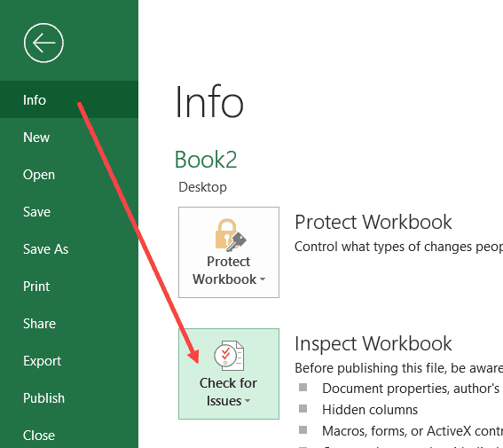


This will show you the total number of hidden rows and columns.

It also gives you the option to delete all these hidden rows/columns. This can be the case if there is extra data that has been hidden and is not needed. Instead of finding hidden rows and columns, you can quickly delete these from this option.
You May Also Like the following Excel Tips/Tutorials:
- How to Insert Multiple Rows in Excel – 4 Methods.
- How to Quickly Insert New Cells in Excel.
- Keyboard & Mouse Tricks that will Reinvent the Way You Excel.
- How to Hide a Worksheet in Excel.
- How to Unhide Sheets in Excel (All In One Go)
- Excel Text to Columns (7 Amazing things you can do with it)
- How to Lock Cells in Excel
- How to Lock Formulas in Excel